Open Research Online
The Open University’s repository of research publications
and other research outputs
Time series forecasting with the WARIMAX-GARCH
method
Journal Item
How to cite:
Corrˆea, J. M.; Neto, A. C.; Teixeira J´unior, L. A.; Franco, E. M. C. and Faria Jr, A. E. (2016). Time series forecasting with the WARIMAX-GARCH method. Neurocomputing, 216 pp. 805–815.
For guidance on citations see FAQs.
c
2016 Elsevier B.V.
Version: Accepted Manuscript
Link(s) to article on publisher’s website:
http://dx.doi.org/doi:10.1016/j.neucom.2016.08.046
Copyright and Moral Rights for the articles on this site are retained by the individual authors and/or other copyright owners. For more information on Open Research Online’s data policy on reuse of materials please consult the policies page.
Author’s Accepted Manuscript
Time series forecasting with the
WARIMAX-GARCH method
J.M. Corrêa, A.C. Neto, L.A. Teixeira Júnior,
E.M.C. Franco, A.E. Faria Jr
PII:
S0925-2312(16)30942-0
DOI:
http://dx.doi.org/10.1016/j.neucom.2016.08.046
Reference:
NEUCOM17480
To appear in:
Neurocomputing
Received date: 7 April 2015
Revised date:
25 October 2015
Accepted date: 18 August 2016
Cite this article as: J.M. Corrêa, A.C. Neto, L.A. Teixeira Júnior, E.M.C. Franco
and A.E. Faria Jr, Time series forecasting with the WARIMAX-GARCH
method,
Neurocomputing,
http://dx.doi.org/10.1016/j.neucom.2016.08.046
This is a PDF file of an unedited manuscript that has been accepted for
publication. As a service to our customers we are providing this early version of
the manuscript. The manuscript will undergo copyediting, typesetting, and
review of the resulting galley proof before it is published in its final citable form.
Please note that during the production process errors may be discovered which
could affect the content, and all legal disclaimers that apply to the journal pertain.
Time series forecasting with the WARIMAX-GARCH method
J. M. Corrêaa*, A. C. Netob, L. A. Teixeira Júniorc, E. M. C. Francod, A. E. Faria Jre
aDepartment of Matematics, Federal Technological University of Paraná, Medianeira, Paraná, Brazil.
bDepartment of Statistic, Federal University of Paraná, Curitiba, Paraná, Brazil.
cLatin American Institute of Technology, Infrastructure and Territory, Federal University of Latin America Integration, Foz do Iguaçu,
Paraná, Brazil.
dDepartment of Electrical Engineering, State University of West Paraná, Foz do Iguaçu, Paraná, Brazil.
eDepartment of Mathematics and Statistics, The Open University, Milton Keynes, Buckinghamshire, England.
Abstract
It is well-known that causal forecasting methods that include appropriately chosen Exogenous Variables (EVs) very often present improved forecasting performances over univariate methods. However, in practice, EVs are usually difficult to obtain and in many cases are not available at all. In this paper, a new causal forecasting approach, called Wavelet Auto-Regressive Integrated Moving Average with eXogenous variables and Generalized Auto-Regressive Conditional Heteroscedasticity (WARIMAX-GARCH) method, is proposed to improve predictive performance and accuracy but also to address, at least in part, the problem of unavailable EVs. Basically, the WARIMAX-GARCH method obtains Wavelet “EVs” (WEVs) from Auto-Regressive Integrated Moving Average with eXogenous variables and Generalized Auto-Regressive Conditional Heteroscedasticity (ARIMAX-GARCH) models applied to Wavelet Components (WCs) that are initially determined from the underlying time series. The WEVs are, in fact, treated by the WARIMAX-GARCH method as if they were conventional EVs. Similarly to GARCH and ARIMA-GARCH models, the WARIMAX-GARCH method is suitable for time series exhibiting non-linear characteristics such as conditional variance that depends on past values of observed data. However, unlike those, it can explicitly model frequency domain patterns in the series to help improve predictive performance. An application to a daily time series of dam displacement in Brazil shows the WARIMAX-GARCH method to remarkably outperform the ARIMA-GARCH method, as well as the (multi-layer perceptron) Artificial Neural Network (ANN) and its wavelet version referred to as Wavelet Artificial Neural Network (WANN) as in [1], on statistical measures for both in-sample and out-of-sample forecasting.
Keywords
Wavelet decomposition, Exogenous variable, ARIMA-GARCH model, Forecasting.
List of adopted acronyms
ARIMA: Auto-Regressive Integrated Moving Average.
ARIMAX: Auto-Regressive Integrated Moving Average with eXogenous variables.
GARCH: Generalized Auto-Regressive Conditional Heteroscedasticity.
ARIMAX-GARCH: Auto-Regressive Integrated Moving Average with eXogenous variables and Generalized Auto-Regressive Conditional Heteroscedasticity.
EVs: Exogenous Variables.
WCs: Wavelet Components.
WARIMAX-GARCH: Wavelet Auto-Regressive Integrated Moving Average with eXogenous variables and Generalized Auto-Regressive Conditional Heteroscedasticity.
ANN: Artificial Neural Network.
WANN: Wavelet Artificial Neural Network.
1. Introduction
There is a vast body of literature on methods and techniques for the modeling and forecasting of time series (see e.g. [2]). One of the most well-known is the class of Auto-Regressive Integrated Moving Average (ARIMA) models proposed by [3] for stationary time series exhibiting linear auto-dependence characteristics. An ARIMA model makes use of available historical data from the underlying time series, denoted by ( ), to quantify any auto-regressive and moving-average patterns and produce forecasts. Many time series are often affected or influenced by certain external factors such as special events (e.g. legislative activities, policy changes, environmental regulations), as well as by uncertain or random events (referred to as stochastic events), that generate data that may be available to be used as Exogenous Variables (EVs). Some models can accommodate one or more such variables to help improving the forecasting process. Box and Jenkins themselves proposed an extension to an ARIMA model, the transfer function model (see e.g. [2]), which can account for EVs. The general exogenous model employed by the ARIMA model has been discussed by [4], where it is referred to as an Auto-Regressive Integrated Moving Average with eXogenous variables (ARIMAX) model. [5] refers to the ARIMAX model as dynamic regression model. Both [4] and [5] show increased forecasting accuracy gains are achieved when EVs are properly used in the modeling process. ARIMAX models, however, require adequate EVs are available and that the underlying time series is stationary (or transformed into a stationary one).
In the conventional ARIMAX model, the conditional variance of its innovations is typically supposed to be constant (homoscedasticity). However, many time series often exhibit periods of unusual high volatility followed by periods of relative stability. In such situations, the constant conditional variance assumption may be considered inappropriate. In order to account for changes in conditional variance (heteroscedasticity), [6], [7], [8], amongst others, developed a class of conditional heteroscedastic models that allows the changing conditional variance (volatility) of a time series to be explicitly modelled. The Auto-Regressive Conditional Heteroscedastic (ARCH) model of [6] allows for the conditional variance to depend on past values of the conditional variance itself; while the Generalized ARCH (GARCH) model of [7] enable the volatility to depend on past values of both the squared innovation and conditional variance itself. The WARIMAX-GARCH method proposed here employs a GARCH model as one of its components. Other extensions of a GARCH model are, for example, the GARCH-in-mean (GARCH-M) of Engle, [9] that includes a heteroscedasticity term into the mean model (represented by either the ARIMA or ARIMAX components); and the Exponential GARCH (EGARCH) model of [10], which models the conditional variance in logarithmic form, that does not require non-negativity constraints and allows for asymmetric effect of information on the volatility. In effect, the GARCH term of the WARIMAX-GARCH method can be chosen to be any of such extensions of a GARCH model depending on the application.
In many practical cases, appropriate EVs are just not available to be employed. For instance, [11] claim that, contrary to price-based management, regression methods are somewhat less common in quantity-based revenue forecasting applications (such as airline and hotel revenue management) because it is often difficult to obtain data on the explanatory EVs as an automated data feed. In such cases, the only explanatory variables that can be used must come from the historical underlying data. In this context, the approach adopted in this paper is to generate WEVs from WCs of the time series to be used as EVs by the WARIMAX-GARCH method as we shall see. This way, it is possible to obtain improved forecasting performance gains similarly to the ones obtained by [5] when using the conventional ARIMAX-GARCH model albeit in another application as we shall see.
Note that, in practical terms, the Wavelet Exogenous Variables (WEVs) can be seen as representing the quantified frequency patterns present in the time series that the usual ARIMAX model does not account for. Now, mathematically, the WEVs consist of the wavelet components (the WCs), where a WC is defined by orthogonal projections of an original time series on orthogonal complete subspaces, called the “wavelet subspaces”, of the
space.
Thus, the WARIMAX-GARCH method consists of a new causal forecasting method that, based on ARIMAX-GARCH models, generates and uses the WCs as exogenous variables (the WEVs). Figure 1 shows a flow diagram with seven levels depicting the steps, described below, of the WARIMAX-GARCH method. To apply the WARIMAX-GARCH method, the underlying time series is first split into a training (in-sample) and a testing (out-of-sample) sample. The training sample, denoted by ( ), where T is a conveniently chosen time period, is decomposed via wavelet decomposition of level r as shown by the top two levels of the diagram in Figure 1. This decomposition produces (for each time ) one WC of approximation at level , denoted by ̃ , and r WCs of detail at levels ,
, …, ( ), denoted by ̃ , ̃ , …, ̃ ( ) , respectively (as represented by the third level at the top of Figure 1). Each WC is then individually modeled by using an ARIMA-GARCH model, generating h-steps-ahead out-of-sample forecasts to its level. The WCs of ( ) with their out-of-sample forecasts are the completed WCs and are denoted by , , , ..., ( ). Those are interpreted here as EVs ( in Figure 1) in an ARIMAX-GARCH model for forecasting the time series ( ), both in-sample and out-of-sample, to its level (conditional mean) and conditional variance. Finally, under Gaussian assumption, the respective predictive intervals are trivially calculated.
time series (training sample) wavelet decomposition of level r WC of detail at level m0 WC of approximation at level m0
...
WC of detail at level m0+(r-1) out-of- sample forecasts out-of- sample forecasts out-of- sample forecasts WEV1 WEV2 WEVr+1 WARIMAX-GARCH model...
in-sample and out-of-sample forecasts of the levels and variances in-sample and out-of-sample predictive intervals....
Figure. 1. Flowchart of the WARIMAX-GARCH method.
This paper is structured as follows. In Section 2, a more in depth review of the wavelet decomposition method and the ARIMAX-GARCH model, which are component parts of the proposed WARIMAX-GARCH method, are presented, as well as the ANN and WANN models used here as benchmark methods; Section 3 formally defines the WARIMAX-GARCH method; while Section 4 shows the main numerical results of the application to a real time series of dam displacement at the Itaipu hydroelectric, in southern Brazil. Finally, Section 5 concludes the paper.
2. Oriented review of the literature
The purpose of this section is to present a brief review of the concepts and methods required to define the WARIMAX-GARCH method that is introduced in Section 3. It also reviews two neural network methods – a conventional Artificial Neural Network (ANN) and the Wavelet ANN (WANN) proposed by [1] – that are used as benchmark methods for comparing forecasting performances in the application described in Section 4.
It starts in Subsection 2.1 by describing the wavelet decomposition of level r, which is the algorithm adopted in initial step of the WARIMAX-GARCH method. This is followed in Subsection 2.2 by the introduction of the ARIMAX-GARCH models that are posteriorly employed to generate out-of-sample forecasts associated with the wavelet components (WCs)
that are used as exogenous variables. Finally, Subsections 2.3 and 2.4 describe the ANN and the WANN forecasting methods, respectively.
2.1 Wavelet decomposition of level r
Let be the collection of all scalar-valued complex infinite sequences ( ) in such that ∑ | | < , where and denote, respectively, the sets of all complex and integer numbers; and assume that the function 〈 〉 of into is the usual inner product (as in [12]). An element ( ) – with 〈 〉 – is a – wavelet function, if the sequence
( ) ( ( ) ), where ( ) x , forms an orthonormal basis for ; and a
member ( ) – with 〈 〉 – consist of a -scaling function, if the sequence
( ) ( ( ) ), where ( ) x , holds: 〈 ( ) ( )〉 , whenever and ; and, if otherwise, 〈 ( ) ( )〉 , where (see e.g.
[13] and [14]). Based on [15], it can be seen that the subset { ( )}{
{ ( )}
of -wavelet and -scaling functions, where is a fixed integer value, is, in fact, an orthonormal basis for . Accordingly, any sequence ( ) in can be orthogonally decomposed, in terms of an orthonormal basis { ( )}{
{ ( )} , as
represented by
∑
, (1)
where ∑ ( ) is the WC of approximation at level of the state , with 〈 ( )〉; and ∑ ( ) is the WC of detail at level
of , with 〈 ( )〉. The orthogonal decomposition in (1) is usually called a wavelet decomposition.
Tautologically, any finite (scalar-valued complex) time series ( ) can be interpreted as an infinite sequence ( ) in , defined as , if { }; and
, if { }. Therefore, any finite time series ( ) can be orthogonally decomposed by the wavelet decomposition in (1).
In practical terms, once it is impossible to model separately all WCs generated by the expansion (1), an adaptation is required to obtain a finite number of components. Thus, according to [16], a good alternative may occur thoroughly by means of the wavelet decomposition of level r of ( ), where and , is given by
̃ ∑ ( ) ̃ , (2) where is the level parameter (which is often assumed to be equal to r); is the approximation error term, that is, the difference between the state and its (wavelet) approximation ̃ ∑ ( ) ̃ (nevertheless, in practice, it is usually assumed that
is equals zero); ̃ ∑ ( ) and ̃ ∑ ( ) ( ),
which are, respectively, WCs of approximation at level and of detail at level and consist, respectively, of the approximations to and , in (1); and is a parameter that takes an integer value such that . If T is not an integer power of 2, the sequence
next integer power of 2. This procedure may be carried out because the zeros added up do not affect the calculation of the WCs ̃ and ̃ generate in (2) (see e.g. [17]), preserving the auto-correlation and its components, in (2), for all t, where .
After obtaining the WCs in (2), that is, ̃ and ̃ ( , ..., ( )), they are individually modeled by an adequate ARIMA-GARCH model in order to produce their out-of-sample forecasts. Finally, the mentioned forecasts complete the WCs in (2), providing the WEVs to be used as exogenous variables by ARIMAX-GARCH models as described in the following section.
Note that the WEVs were not modeled individually by ARIMA models as those models cannot map non-linear auto-dependence that is often present in the WCs. Further to that, the WCs of detail usually present conditional heteroscedasticity (as is the case of the time series modeled in this paper). Therefore, ARIMA-GARCH models have been chosen for mapping both linear and non-linear effects in the WCs and obtain more accurate in-sample and out-of-sample forecasts of the WCs, in particular of the detail WCs. Consequently, the in-out-of-sample and out-of-sample forecasts that can be interpreted as aggregators of information from different sources (namely, the different ARIMA-GARCH models used to model the WCs) to the original time series will contain both linear and non-linear information.
2.2 The ARIMAX-GARCH model
Let ( ) be a stationary time series (or a non-stationary time series that can be transformed into a stationary one) that exhibits linear auto-dependence. Also, assume
(( ) ( ( ) ) ) denotes a list of vectors of realizations from stationary exogenous variables of ( ). Based on [4] and [5], each realization can be represented by an ARIMAX (p, d, q) model, with the mathematical formulation:
∑ ∑ ∑ ∑ , (3)
where B is the backward operator defined by , with k belonging to ;
( ) is the difference operator, with d representing its order; ( )
and ( ) are
the ordered lists of model complex parameters, with and , and ( ) is the ith ordered list of complex model parameters associated with the exogenous component (these three lists of parameters need to satisfy both the invertibility and the stationarity conditions - see e.g. [18] and [19]); is an innovation consisting of a state of the random variable from an uncorrelated stochastic process with zero mean; p and q are, respectively, the orders of the Auto-Regressive (AR) part ∑ (AR(p)) and of the Moving Average (MA) part ∑ (MA(q)); and, is the maximum lag order in the sum ∑ of the
exogenous variable , with ( ). Particularly, if , for all (
) and all =0…, , then the model in (3) above becomes a conventional ARIMA (p, d, q). Note that, a SARIMAX (p, d, q) x ( ) model - also known as a multiplicative ARIMAX (p, d, q) model – can be used for modeling a seasonal time series (as in [18]). It generically consists of an ARIMAX model with seasonal components (please, see Section 3 for details).
In equation (3) above, it is assumed that the innovation term is a realization of an uncorrelated random variable , with zero mean and constant conditional variance, that is, , for all t. However, many time series do not satisfy this stationarity condition (called
homoscedasticity). In some cases, the changing conditional variance (volatility) may depend on past squared innovations of the time series or past values of the variance itself such that an ARMA structure, as well as an extension of it, can be adopted for temporally projecting the volatility. This way, unconditionally, the variance is constant, but conditional on past values it is allowed to change in time. According to [20], the general GARCH ( , ) model for the conditional variance of the innovation is given by
∑ +∑ , (4)
where the following constraints must hold: ∑ +∑ ; ; ( ) and ( ). Equation (4) is used by the WARIMAX-GARCH method to generate in-sample and out-of-sample forecasts of the conditional variance of the time series
( ). In addition, multiplied by a parameter can be used in (3) to account for a non-linear effect to construct the forecasting of its level (conditional mean). Notice that the generating mechanism for a GARCH innovation process ( ) is defined by
, where: is a realization of a standardized, independent and identically distributed random variable ; and is the conditional standard deviation.
A model compounded by (3) and (4), which accounts for the above mentioned constraints, is called an GARCH model. In order to obtain the best possible ARIMAX-GARCH model, three basic steps should be carried out: (i) test the plausible values for the parameters
p, d, q and , in (3), as well as the parameters and in (4) (which can be obtained through the profile analysis of the plots of simple and partial auto-correlation functions of the ordinary standard innovations ( ) and the squared standard innovations ( ), as described by [20] and [6]; (ii) define the method to be used to estimate the ARIMAX-GARCH parameters - the most common is the Maximum Likelihood Estimation (MLE) method (as in [18]); and, (iii) make a diagnostic check to choose the most parsimonious and adequate model to be used for generating both the in-sample and the out-of-sample forecasts of ( ) and their volatilities.
It is worth pointing out that similarly to the way that the h-steps ahead out-of-sample forecasts of conditional means are produced (for instance, through an estimated ARIMAX model), the h-steps ahead forecasts of conditional variances (volatilities) are generated by means of an estimated GARCH model (or an extension of it). For more details, please see [18], wherein a GARCH-in-mean model produces out-of-sample forecasts of volatilities and employs them in the construction of the forecasts for the corresponding conditional means. In fact this approach aims to aggregate non-linear information (coming from the squared auto-dependence exhibited by a given time series) from the forecasts of the conditional means in order to increase its predictive accuracy. Note that the WARIMAX-GARCH method proposed here can adopt any GARCH approach to forecast volatilities.
2.3 Artificial Neural Networks
Artificial Neural Networks (ANNs) are well known to be flexible computing frameworks for modeling and forecasting a broad range of stochastic time series exhibiting either linear or non-linear auto-dependence structures. Contrary to many linear statistical forecasting models, stationarity is not required by ANN methods (see e.g. [1]). Another important aspect of ANNs is that they are universal approximates of compact (i.e., closed and bounded) support functions, as showed in [21]. In effect, since observations from a time series ( ) that exhibit dependency on past values may be seen as points of the domain of an unknown
compact support function, it follows that the ANNs are capable of approximating them (for modeling or forecasting) with a high degree of accuracy. According to [22], the predictive power of ANNs comes from the parallel processing of the information exhibited by the data. In addition, AAN models are largely determined by the stochastic characteristics inherent in the time series.
In this context, the feed-forward multi-layer perceptron ANNs (see e.g. [23]) are the most widely used neural prediction models for time series forecasting. Particularly, a single hidden layer ANN (henceforth, for simplicity, referred to as ANN) is characterized by an artificial network composed by three layers (namely, input, hidden an output layers) of simple processing units numerically connected by acyclic links. The relationship between the output and the L-lagged inputs, ( ), has the following mathematical representation
∑ ( ∑ ) , (5)
where ( ) and ( ) are the ANN parameters, called connection weights; is the number of input nodes; is the number of hidden nodes; is the approximation error at time t; and ( ) is the transfer function, here, a logistic function - although it is possible to adopt other functions (see e.g [23]). The logistic function is widely employed as the hidden layer transfer function in neural network forecasting and is mathematically defined by
( ) ( ) , (6)
where ∑ and ( ) is the exponential function with Euler’s basis (as in [23]). Due to ( ) being a non-linear transfer function, the ANN model in (5), in fact performs a non-linear mapping of the past observations ( ) to produce a forecast for . In general, the model in (5) can be rewritten, as
( ) , (7)
where denotes a vector of all ANN parameters and ( ) is the model determined by the network structure and the connection weights in (5). Note that the neural network as defined above is equivalent to a non-linear auto-regressive model.
In practice, is unknown and hence needs to be numerically determined. So, in order to find its estimated value, ̂, that accounts for some criteria (an objective function), an optimization algorithm is applied to training data. Although there are several methodologies available in the literature, we adopt, in line with [23], the Levenberg-Marquardt’s algorithm. The minimization of the in-sample sum of squared errors (i.e., ∑ ) is the numerical criteria of this ANN. Once ̂ is determined we have that
( ̂) ̂ (8)
with ( ̂) ̂ consisting of the optimized ANN outcome at time t, which is the forecast of the state , and ̂ being the forecasting error of ̂ .
2.4 Wavelet Artificial Neural Networks
There is currently a number of distinct wavelet decomposition methods combined with ANNs (referred to as wavelet ANNs) that are used for time series forecasting and achieve
remarkable accuracy gains. In fact, there are several studies showing the predictive accuracy gains achieved by wavelet ANN methods such as in [24], [25], [26] and [1] amongst others. Nevertheless, due to the remarkable results achieved in their experiments involving the forecast of the non-stationary solar radiation time series, the [1]’s wavelet ANN method (henceforth referred to as wavelet ANN method) was chosen to be used as a benchmark method in this paper.
For a time series ( ), the wavelet ANN method is carried out in two steps:
Step 1: a wavelet decomposition of level (as in Section 2.1) of ( ) is performed, producing 1 WC of approximation at level , denoted by
( ), where , and WCs of detail at levels , , …, ( ), denoted by ( ), respectively, where ; and
Step 2: The WCs from Step 1 are simultaneously modelled through the ANN described in Section 2.3 producing forecasts similarly to (8), as follows:
(
( ) ̂) ̂ (9)
where (
) and ( ), notice that , , …, ( ) are the input data. Similarly to the ANN in (8), the optimal solution ̂ in (9) is obtained via Levenberg-Marquardt’s algorithm such that ∑ is determined. The forecast of is
(
( ) ̂) ̂ , and ̂ is the forecasting error of ̂
(please, see [1], for more details).
3. The WARIMAX-GARCH method
The ARIMAX-GARCH model requires that EVs are available to be used. In cases, where EVs are not available, an ARIMA-GARCH model can be used but at the expense of a likely lower predictive accuracy. The WARIMAX-GARCH method defined below aims to, at least in part, address this problem. The general steps, mentioned at the end of Section 1, are described in more detail as the following five steps.
Step 1: a wavelet decomposition of level r (described in Section 2.1) of the underlying time series ( ) is performed, generating WCs. That is, one WC of approximation at level , denoted by ̃ ( ), and r WCs of detail at levels from to ( ), denoted by ̃ ( ) for m=m0, …, m
0+(r-1);
Step 2: each WC obtained in Step 1 is individually modeled by using a distinct ARIMA-GARCH in order to generate their out-of-sample forecasts;
Step 3: the WCs of the Step 1 are completed by their out-of-sample forecasts (of horizon h) of the Step 2, producing the Completed WCs (CWCs) consisting of the wavelet EVs (WEVs). Algebraically, they are given by the data sets below:
̃ or ( ) consist of the CWC of
approximation at level of ( ) and is such that: ̃ ̃ , if ; and ̃ ̂ , if -
where ̂ represents the out-of-sample forecast at instant t generated by an ARIMA-GARCH in Step 2;
̃ or ( ), where i=2,…, r+1, consists of
the CWCs of the detail at level , where ( ), of
( ) and is such that: ̃ ̃ , if ; and
̃ ̂ , if - where ̂ denotes the out-of-sample forecast at time t produced by an ARIMA-GARCH in Step 2.
Step 4: the CWCs generated in Step 3 are treated as wavelet exogenous variables by the following WARIMAX-GARCH (p, d, q) x (P, D, Q) model to generate in-sample and out-of-sample forecasts to the level and the conditional variance of ( ), as well as their predictive intervals, under the assumption of Gaussian innovations out of sample.
A WARIMAX-GARCH (p, d, q) x (P, D, Q) model is mathematically defined by (10) and (11) below as ( ) ( ) ( ̃ ) ∑ ̃ ( ) ( ) ( ) , (10)
where the components ( ):=( ), ( ) (
), ( ) , ( ) , ( ) ( ) and
( ):=( ), are the polynomials associated with a conventional SARIMA(p, d, q) x (P, D, Q) model; is the parameter linearly associated with the conditional variance ; and are the parameters linearly associated with ̃ and ̃ , respectively. In turn, ( ) is either the
identity or a logarithmic function - which is very useful, in many cases, to turn the level of a time series constant (as in [18]) as well as to improve forecasting performance. Finally, , for and , is the difference operator associated
( ) that (as in [18]) can be used to generate a new time series with constant mean. It is worth pointing out that and can assume different orders when one is searching for the optimal model.
Concerning the parameters of the WARIMAX part, they require assumptions similar to those required by the parameters of the conventional ARIMAX and are estimated here by Maximum Likelihood method. In order to obtain the model’s conditional variance for ( ), the WARIMAX-GARCH model uses its GARCH ( ) component, which is, in the strict sense, given by
∑ +∑ , (11)
where , with being the realization of a standardized, independent and identically distributed random variable and the conditional standard deviation.
Step 5: once the collection of in-sample and out-of-sample forecasts
̂ ( ) of the level of ( ), as well as of their volatilities ̂ ( ) are determined, the prediction intervals
[ ̂ ̂ ] ( ), with any 1- level of confidence,
under the assumption of Gaussian innovations, can be determined straightforwardly. The inferior limit ̂ and the superior limit ̂ of the prediction intervals at any time t are, respectively, defined by ̂ ̂ ̂ and ̂ ̂ ̂ , where represents a state of a random variable associated with .
Note that although wavelet methods are applicable to non-stationary and/or non-linear time series (as in [14]), all WEVs of a WARIMAX-GARCH model should be stationary to satisfy this requirement of the ARIMAX modelling approach. However, non-stationary WEVs formatted by the WC of approximation ̃ ( ) and its lagged versions, can be made stationary via differencing with the use of the back shift operator and/or by transforming with the mapping ( ) associated with the component, as is usually done in ARIMA modelling when the original series is non-stationary.
Also note that, WEVs consisting of WCs of detail, as well as their stationary versions, are always stationary in level such that a difference operator in (5) is applied just to help achieve improved forecasting performances and/or obtain a plausible model. In fact, according to [14], a wavelet function at level , ( ), consists of a short duration curve which image values have zero mean. Furthermore, a Wavelet Component (WC) of detail at level , ̃ ( ), is mathematically defined by a linear combination of wavelet
functions at level such that ̃ ∑ ( ) ( ), for each time t, where
. Similarly to ( ), a WC of detail ̃ takes values around zero; from the statistical point of view, it means that ̃ exhibits stationarity in the conditional mean (level). Now, based on [14], since is a fixed parameter associated with the spectral frequency of ̃ , it follows that its conditional variances (or volatilities) have stationary stochastic fluctuation. Therefore, a WC of detail at level will always be stationary.
4. Empirical results
In this section, the main results of an application of the WARIMAX-GARCH method to a daily time series of the Itaipu dam displacement measures is described. For comparative purposes, ARIMA-GARCH models, as well as an ANN and a Wavelet ANN method (as in [1]) were also applied to the displacement series. In Section 4.1, the series is described and an initial statistical analysis conducted to justify the selected models. In Section 4.2, the ARIMA-GARCH models to be applied to the displacement series are identified. Section 4.3 shows the five basic steps of the applied WARIMA-GARCH method together with the main statistical tests used for its validation. Section 4.4 concludes with a comparative analysis showing the effectiveness of the proposed method in terms of forecasting performances relative to the ARIMA-GARCH, ANN and Wavelet ANN models.
4.1 The daily series of Itaipu dam displacement
A time series of physical displacement of the dam that supplies the Itaipu hydroelectric plant in southern Brazil is modeled due to its relevance and statistical properties. The Itaipu dam is the world’s most powerful dam with a length of 170 Km and an average width of 7 Km, reaching an area of 1350 Km2, and allowing electricity generation in excess of 90 billion KWh. It supplies 93% of the energy consumed by Paraguay and 20% of the Brazilian consumption. Please refer to http://www.aboutcivil.org/itaipu-dam-design-construction-facts.html for more information about the Itaipu dam. Monitoring and forecasting the dam’s physical displacements allow engineers to take corrective actions to prevent structural damage and accidents that can lead not only to interruptions of electricity generation but also to failures of more serious consequences. The data in this application come from automatic measurements of displacement taken at daily intervals in the period from 28th October 2005 to 24th October 2012. Figure 2 shows the time plot of the corresponding 2554 daily observations. The initial 2506 observations were used as in-sample training and the last 48 observations were used as out-of-sample for model testing. Note that there were no exogenous variables, such as dam levels and water pressure measurements, available for use in the application. In fact, there is no other data available (of enough quality) than the dam displacement time series that could be used in the modeling process.
Figure. 2. The daily time series of dam displacement at the Itaipu electricity plant.
8 9 10 11 12 13 14 1 401 801 1201 1601 2001 2401 Dam d isp lac e m e n t Time
It can be seen from Figure 2 that there are both high and low frequency oscillations in the displacement data. Although a seasonal ARIMA model can capture the low-frequency variations, it would not be able to deal with the high-frequency ones at all. A WARIMAX-GARCH model however can model the high-frequency oscillations in the underlying series time through the ARIMA-GARCH models integrated with the wavelet decomposition approach.
An Augmented Dikey-Fuller (ADF) unit root test was conducted and did not reject, at 1% significance level, the hypothesis of non-stationarity of the displacement data. Nevertheless, the ADF strongly rejected non-stationarity, at 1% level, of the purely log-transformed version, as well as tautologically of the second difference of the log-transformed series. The second difference here was not used to get stationarity, but also for reaching improved accuracy gains. The simple and partial auto-correlation functions relative to this last one, as well as its squared version, showed significant values, at 1% level – what supports the choice of an ARIMA and GARCH modeling. Therefore, since there were no conventional exogenous variables available to be used by the ARIMAX-GARCH model in this application, it follows that an ARIMA-GARCH model was consider plausible for modeling process.
The investigation conducted in this section generated multi-step in-sample and out-of-sample (point and interval) forecasts from both an ARIMA-GARCH model (used as a benchmark model) and the WARIMAX-GARCH method. Residual diagnostics for statistical validation were conducted using augmented Dickey-Fuller unit root tests, Ljung-Box and Durbin-Watson tests for first order auto-correlation, as well as ACF and PACF plots, BDS tests to detect non-linear serial auto-correlations and ARCH tests for unconditionally constant residual variance (see e.g. [18]). The EViews 8 software was used to perform the tests above. 4.2 The ARIMA-GARCH model
An ARIMA (2, 1, 1) method integrated with the GARCH (2, 1) model (that is, an ARIMA-GARCH (2, 1, 1) x (2, 1) model), with Generalized Error Distribution (GED) (see e.g. [27]), was identified to produce the best fit to the log-transformed double-differenced training sample of dam displacement, ( ). The parameters of that model were estimated by MLE and were statistically significant at 1% level (as can be seen in Appendix A).
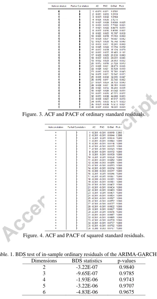
Among all plausible models ARIMA-GARCH obtained from the training sample, the ARIMA-GARCH (3, 2, 4) x (2, 1) produce the more accurate forecasts to the level of the underlying time series, in terms of the in-sample MAPE and MAE. Note that the results of the Ljung-Box (Q-Stat) test applied to the standard residuals of ARIMA-GARCH (3, 2, 4) x (2, 1), shown in Figures 3 and 4, suggest that there is no significant linear auto-dependence (at 1% level) in both the ordinary and the squared standard residuals up to lag 36 (corresponding to three years). In addition, an ARCH test was also conducted and confirmed that there is no significant auto-correlations in the residual variance (at 1% level) from lags 1 to 36. Furthermore, the calculated Durbin-Watson statistic of 2.092367 suggests there is no significant auto-correlation of lag 1 in the ordinary standard residuals. Please see Appendix A for more detail of tests performed and to [18] for more information on the statistical techniques behind those tests.
Figure. 3. ACF and PACF of ordinary standard residuals.
Figure. 4. ACF and PACF of squared standard residuals.
Table. 1. BDS test of in-sample ordinary residuals of the ARIMA-GARCH model. Dimensions BDS statistics p-values
2 -3.22E-07 0.9840 3 -9.65E-07 0.9785 4 -1.93E-06 0.9743 5 -3.22E-06 0.9707 6 -4.83E-06 0.9675
Table 1 shows the statistics and the corresponding p-values for dimensions 2 to 6 of a BDS test (which consists of a statistical test used to verify the existence of linear and non-linear
auto-dependence existing in a data set (see e.g. [28])) applied to the in-sample residuals of the ARIMA-GARCH (3, 2, 4) x (2, 1) model. According to those p-values it is possible to conclude that there is no evidence at 1% level of significance, in all five dimensions, of both linear and non-linear auto-dependences in the in-sample forecasting errors. In particular, the linear and squared auto-dependences previously present in the forecasting residuals have been properly mapped by the ARIMA-GARCH models specified above. Therefore, the in-sample forecasting residuals can be considered as a white noise process with zero mean.
It is worth mentioning that model selection among all identified plausible ARIMA-GARCH models was determined by comparing the forecasting performances of each candidate model as measured by their Absolute Percentage Error (APE), Mean Absolute Percentage Error (MAPE), Mean Absolute Error (MAE) and . The selected best model, the one with the smallest APE, MAPE and MAE and with the largest R2, is described in the following section.
4.3 The WARIMAX-GARCH model
The first step of the WARIMAX-GARCH method was implemented in MATLAB (version 2013a). A wavelet decomposition of level 2 was obtained from the training sample of the dam displacement data. The plots of the WCs, with orthonormal basis db40 (as described in [29]), can be seen in Figure 5.
(a) WC of approximation at level 2, ̃ ( ).
(b) WC of detail at level 2, ̃ ( ).
(c) WC of detail at level 3, ̃ ( ).
Figure. 5. WCs from the training sample of the dam displacement data set.
Recall from (2) that, for this application, ̃ ̃ + ̃ ( ), where is a null error (that is, ). In Step 2 of the WARIMAX-GARCH method, each one of the WCs ̃ , ̃ and ̃ ( ) were individually modeled by three different ARIMA-GARCH models (which details are shown in Appendix B), providing the sequence of the out-of-sample forecasts to their respective levels, namely ̂ , ̂ and
̂ ( ). The forecasting horizon was chosen as (i.e., 48 days-ahead). All estimated parameters of the three models were statistically significant, at 1%, and the residual diagnostics confirmed their plausibility (as shown in Appendix B).
In Step 3, the three CWCs ̃ , ̃ and ̃ (or and , respectively) consist of the WEVs generated from the dam displacement series. As mentioned before, they are easily obtained by filling in the WCs with their out-of-sample forecasts produced in the Step 2. Algebraically, it means that
I. ̃ (( ̃ ) ( ̂ ) ); II. ̃ (( ̃ ) ( ̂ ) ); and III. ̃ (( ̃ ) ( ̂ ) ).
In Step 4, using the WEVs ( ) ( ), the WARIMAX-GARCH model was adjusted and then used to generate 48-steps-ahead forecasts to the level and the conditional variance of the underlying series. Algebraically, the forecasting formulation of the best WARIMAX model obtained is given in (12).
( ) ( ) ∑ ̃ ̃ ̃ . (12)
In Appendix B, the estimated WARIMAX model above together with its main statistics can be seen in more detail. Note that all three WEVs, , and , were required in the best WARIMAX model above. In addition, the volatility provides a non-linear effect to represent the state . Also, the best GARCH model was a GARCH (1, 1) with GED distribution, with the following algebraic formulation
+ .
Its estimates and main statistics can also be seen in Appendix B. The MLE method was used to obtain all estimates of the best WARIMAX-GARCH model parameters. Appendix C shows that all estimates are statistically significant, at 1%.
Figures 6 and 7 show, respectively, the ACF and the PACF (from lags 1 to 36) of both the ordinary and the squared standard residuals from the estimated WARIMAX-GARCH model. Note that all estimated ACF and PACF fall within the 99% confidence intervals suggesting those values were all non-significant. The Ljung-Box (Q-Stat) statistics on those figures also suggest there are no significant linear auto-dependences (at 1% level) in the in-sample ordinary and squared standard residuals of the WARIMAX-GARCH model. Also, note the ARCH test, (Prob) in Figure 7, confirmed there is no ARCH effect in the forecasting residuals. The Durbin-Watson statistic was 2.026328 confirming the lack of first-order auto-correlation of those in-sample standard residuals (please see Appendix C for more details).
Figure. 6. ACF and PACF of ordinary standard residuals.
Figure. 7. ACF and PACF of squared standard residuals.
Table. 2. BDS test of in-sample ordinary residuals of the WARIMAX-GARCH model. Dimensions BDS statistics p-values
2 -3.22E-07 0.9840 3 -9.65E-07 0.9785 4 -1.93E-06 0.9743 5 -3.22E-06 0.9707 6 -4.83E-06 0.9675
Based on the p-values in Table 2, it can be concluded that there is no strong evidence (at 1% level) of both the linear or non-linear auto-dependence structure in the in-sample ordinary
standard residuals in all dimensions. Particularly, the linear and squared auto-dependence previously structures existing in them have been properly mapped by the adopted WARIMAX-GARCH model above. Therefore, the in-sample forecasting residuals can be considered as a white noise process with mean of zero, validating the WARIMAX-GARCH model.
4.4 ANN and WANN methods
As for the ANN and WANN methods, an iterative computational algorithm was used to test values for the ANN and WANN parameters and to choose their optimum values. The tested ANN parameters were the number of window lengths ( ) (i.e., ), of neurons ( ) in hidden layer (i.e., ) and, in the case of Wavelet ANN method, of the null moments ( ) of the Daubechies wavelet functions (as in [14]) for each WC, (i.e., ). In order to avoid excessive processing time, the following parameters were kept as fixed: premnmx normalization (as in [23]); one hidden layer; hyperbolic tangent and linear activation functions at the hidden and output (endowed with one neuron) layers, respectively; Levenberg-Marquardt training algorithm (for details about the mentioned ANN parameters, please, see [23]); and, in the case of Wavelet ANN method, (i.e., wavelet decomposition of level 2), following the [1]’s approach. So, Table 3 exhibits the obtained optimal parameters of both the ANN and WANN methods.
Table. 3. Optimal ANN and WANN parameters.
METHOD Parameters Optimal values Wavelet Component
ANN 4 - 2 - Wavelet ANN 6 Approximation at level 2 3 1 2 Detail at level 2 2 1 2 Detail at level 3 3 1
4.5 Comparative of forecasting performances
Table 4 shows the MAPE and the MAE statistics for the in-sample and the out-of-sample forecasting performances of the three benchmark methods (namely, the ARIMA-GARCH, ANN and WANN approaches) and the WARIMAX-GARCH models. The optimal ARIMA-GARCH model obtained in Section 4.3 is an ARIMA-ARIMA-GARCH (3, 2, 4) x (2, 1).
It can be seen from the results in Table 4 that the WARIMAX-GARCH method had smaller MAPE and MAE values, and thus, better performances than the ARIMA-GARCH, ANN and WANN models both for the in-sample and out-of-sample periods. In particular, the WARIMAX-GARCH method produced greater improvements in out-of-sample forecasting performances, with 0.899% of MAPE and 0.1065 of MAE against 1.840% of MAPE and 0.2216 of MAE for the best benchmark method - i.e., WANN model (an improvement in excess of about 52% in both counts). It appears from those results that the use of WCs implied in significant forecasting performance improvements both in-sample and (in particular)
out-of-sample. In other words, the WARIMAX-GARCH has better modeled the dynamics of the referred time series and produced better forecasts than the WANN method.
Table. 4. The in-sample and out-of-sample forecasting performances.
METHODS MAPE MAE
In-sample Out-of-sample In-sample Out-of-sample
WARIMAX-GARCH 0.300% 0.899% 0.0338 0.1065 ARIMA-GARCH (benchmark I) 0.398% 5.324% 0.0448 0.6368 ANN (benchmark II) 0.425% 2.247% 0.0474 0.2710 Wavelet ANN (benchmark III) 0.438% 1.840% 0.0495 0.2216
Figure 8 shows the plot of the Absolute Percentage Errors (APEs) calculated for the out-of-sample forecasts at each step-ahead by both models. Note that the WARIMA-GARCH model not only had lower APEs than the ARIMA-GARCH model for each step-ahead forecast from 1 to 48, but also produced comparatively better forecasts for larger steps-ahead. In fact, while the forecasting errors of the ARIMA-GARCH model showed a positive trend (growing from just under 1% to about 9%) the WARIMAX-GARCH showed fluctuations along the 1% line with increases in the forecasting horizon. Appendix B shows other plots of the temporal evolution of out-of-sample observations and the respective forecasts from both methods to support the conclusion that, in fact, the WARIMAX-GARCH model has a better power of generalization.
Figure. 8. Comparison of temporal evolution of APEs obtained from the WARIMAX-GARCH and ARIMA-WARIMAX-GARCH methods.
Figure 9 also exhibits the plot of APEs calculated for the out-of-sample forecasts at each step-ahead by both methods. From step 20, it can be seen that the WARIMAX-GARCH method has obtained remarkably better forecasting accuracy than the Wavelet ANN (the
0.00% 1.00% 2.00% 3.00% 4.00% 5.00% 6.00% 7.00% 8.00% 9.00% 10.00% 1 4 7 10 13 16 19 22 25 28 31 34 37 40 43 46 A PE
Forecasting horizon (steps-ahead)
WARIMAX-GARCH ARIMA-GARCH
second best method), accounting for the best forecasting performance amongst all the benchmark methods in Table 4.
Note that, similarly to the ARIMA-GARCH model, the WANN method have lost accuracy for larger forecasting horizons, while the WARIMAX-GARCH has retained its forecasting performance.
Figure. 9. Comparison of temporal evolution of APEs obtained from the WARIMAX-GARCH and WANN methods.
Figures 10 (a) and (b) show the plots of the actual observed displacements together the point forecasts and associated 99% upper and lower forecasting limits by (a) the ARIMA-GRACH model and (b) the WARIMAX-GARCH method. Notice that in Figure 10 (a) the forecasts by the ARIMA-GRACH model were all larger than the observed values at each time, however all within the 99% prediction intervals.
On the other hand, in Figure 10 (b), the forecasts by the WARIMAX-GARCH method tracked the trend in displacement more closely and also were all within the 99% prediction intervals which limits were much smaller than those of the ARIMA-GARCH model. That is, the variance of the predictive density from WARIMAX-GARCH was lesser. This plot also shows the dynamics of the forecasts produced by the WARIMAX-GARCH method that tried to project the oscillations of the displacements into the ‘future’.
0.00% 0.50% 1.00% 1.50% 2.00% 2.50% 3.00% 3.50% 4.00% 4.50% 5.00% 1 5 9 13 17 21 25 29 33 37 41 45 M A PE
Forecasting horizon (steps-ahead)
WARIMAX-GARCH Wavelet ANN
(a) ARIMAX-GARCH Method.
(b) WARIMAX-GARCH method.
Figure. 10. Forecasts (with prediction intervals) and observed displacements.
In terms of the coefficient, which is used to measure the amount of variation in the time series that is explained by the estimated method, the ARIMA-GARCH model had
and the WARIMAX-GARCH method had . Those results show the WARIMAX-GARCH explained approximately 99.72% of the variations in the time series of Itaipu dam displacements, while the ARIMA-GARCH only explained 36.14%.
5. Conclusions
In this paper, a new causal forecasting method called the WARIMAX-GARCH method is proposed that incorporates wavelet variables (obtained from wavelet decomposition of the underlying series) treated as exogenous variables incurring in substantial improvements in
8.00 9.00 10.00 11.00 12.00 13.00 14.00 15.00 16.00 17.00 18.00 1 6 11 16 21 26 31 36 41 46 D isp lac e m e n t Time Inferior limit Superior limit Observations Forecasts 11.10 11.30 11.50 11.70 11.90 12.10 12.30 12.50 1 6 11 16 21 26 31 36 41 46 D isp lac e m e n t Time Inferior limite Superior limite Observations Forecasts
forecasting performances over traditional ARIMA-GARCH, ANN and Wavelet ANN models. The incorporated wavelet components have good statistical properties to be used as exogenous variables by the WARIMAX-GARCH method. For instance, the detail components are always a second-order stationary process (usually required from exogenous variables that integrate a linear statistical regression model) and also always exhibit conditional variance (volatility) – similarly to a number of the financial time series (see e.g. [6]) – that enables nonlinear effects to be accounted for in the final model. Also, the approximation wavelet component can always be modeled by an ARIMA-GARCH model whenever the original underlying time series can also be. Furthermore, it can be easily seen that WCs always show strong correlations with the response variable they are obtained from.
The proposed method was applied to a daily time series of dam displacement in southern Brazil. Comparative results against the ARIMA-GARCH model showed the WARIMAX-GARCH method not only to produce significantly improved point forecasting performances but also improved predictive accuracy as measured by the prediction intervals that are straightforwardly operationally obtained. In addition, the WARIMAX-GARCH model has achieved considerably better forecasting performance than both the ANN and Wavelet ANN methods in the Itaipu dam displacement application.
This methodology has also been applied to other time series with similar results and will be subject of a future publication.
Acknowledments
The authors would like to express gratitude for the support provided by the Itaipu hydroelectric company, the Post-graduate Program in Numerical Methods in Engineering (PPGMNE), the Center for Advanced Studies in Dam Safety (CEASB), the Itaipu Technological Park (PTI), the Coordination for the Improvement of Higher Education Personnel (CAPES) of the Brazilian Education Ministry, and, finally, the reviewers for their contributions for the improvement of the paper.
References
[1] L.A. Teixeira Júnior, R.M. Souza, L.M. Menezes, K.M. Cassiano, J.F.M. Pessanha, R.C. Souza, Artificial Neural Network and Wavelet decomposition in the Forecast of Global Horizontal Solar Radiation, Sobrapo. 35 (2015) 1–16.
[2] C. Chatfield, The Analysis of Time Series: an Introduction., Chapman & Hall/CRC, 6th ed., 2004.
[3] G.E. Box, G.M. & Jenkins, Time Series Analysis: Forecasting and Control, Holden-Day, Oakland, Califórnia, 1970.
[4] G.E.P. Box, G.C. Tiao, Intervention Analysis with Applications to Economic and Environmental problems, J. Am. Stat. Assoc. 70 (1975) 70–79.
[5] A. Pankratz, Forecasting with Dynamic Regression Models, Wiley-Interscience., 1991.
[6] R.F. Engle, Autoregressive Conditional Heteroscedasticity with Estimates of the Variance of United Kingdom Inflation, Econometrica. vol. 50 (1982) 987–1007.
[7] T. Bollerslev, Generalized autoregressive conditional heteroskedasticity, J. Econom. 31 (1986) 307–327.
[8] T. Bollerslev, E. Ghysels, Periodic autoregressive conditional heteroscedasticity, J. Bus. Econ. Stat. 14 (1996) 139–151.
[9] R. Engle, D. Lilien, R. Robins, Estimating time varying risk premia in the term structure: The ARCH-M model, Econometrica. 55 (1987) 391–407.
[10] D.B. Nelson, Conditional Heteroscedasticity in Asset Returns: A New Approach, Econometrica. 59 (1991) 347–370.
[11] T.T. Kalyan, J. van R. Garrett, The Theory and Practice of Revenue Management, Springer, 2006.
[12] C.S. Kubrusly, The Elements of Operator Theory, 2nd edn, Birkhäuser/Springer, New York, 2011.
[13] N. Levan, C.S. Kubrusly, A wavelet “time-shift-detail” decomposition, Math. Comput. Simul. 63 (2003) 73–78.
[14] S. Mallat, A Wavelet Tour of Signal Processing: The Sparse Way, Third Edit, 2008.
[15] C.S. Kubrusly, N. Levan, Abstract Wavelets Generated by Hilbert Space Shift Operators, Adv. Math. Sci. Appl. 14 (2006) 643–660.
[16] D.L. Donoho, J.M. Johnstone, Ideal spatial adaptation by wavelet shrinkage, Biometrika. 81 (1994) 425–455.
[17] E. Haven, X. Liu, L. Shen, De-noising option prices with wavelet method, Eur. J. Oper. Res. 222 (2012) 104–112.
[18] J. Hamilton, Time Series Analysis, Princeton University Press, 1994.
[19] H. Lutkepohl, New Introduction to Multiple Time Series Analysis, Springer, 2006.
[20] T. Bollerslev, Generalized Autoregressive Conditional Heteroscedasticity, J. Econom. 31 (1990) 307–327.
[21] G. Cybenko, Approximation by superpositions of a sigmoidal function, Math. Control. Signals, Syst. 2 (1989) 303–314.
[22] G.P. Zhang, Time series forecasting using a hybrid ARIMA and neural network model, Neurocomputing. 50 (2003) 159–175.
[23] S.S. Haykin, Redes Neurais - 2ed., 2o ed., Bookman, Porto Alegre, 2001.
[24] H. Liu, H.Q. Tian, C. Chen, Y. Li, A Hybrid Statistical Method to Predict Wind Speed and Wind Power, Renew. Energy. 35 (2010) 1857–1861.
[25] B. Krishna, R.Y.R. Satyaji, P.C. Nayak, Time Series Modeling of River Flow Using Wavelet Neural Networks, J. Water Resour. Prot. 3 (2011) 50–59.
[26] K.K. Minu, M.C. Lineesh, J.C. Jessy, Wavelet Neural Networks for Nonlinear Time Series Analysis, Appl. Math. Sci. 4 (2010) 2485–2495.
[27] L.M. Liu, Time Series Analysis and Forecasting, Scientific Computing Associations, 2006.
[28] J.D. Hamilton, Causes and Consequences of the Oil Shock of 2007-08, (2009). http://www.nber.org/papers/w15002 (accessed May 2, 2015).
[29] I. Daubechies, Orthonormal bases of compactly supported wavelets, Commun. Pure Appl. Math. 41 (1988) 909–996.
Jairo Marlon Corrêa received the B.S. degree in Mathematics from State University of West Paraná, Foz do Iguaçu, Paraná, Brazil, in 2003; and M.S. degree in Numerical Methods in Engineering from Federal University of Paraná, Curitiba,
Brazil, in 2007. Currently, he is a Ph.D. student in Numerical Methods in Engineering from Federal University of Paraná, Curitiba, Brazil, as well as a professor in Federal Technological University of Paraná, Medianeira, Paraná, Brazil. His research interests include stochastic processes, time series forecasting, machine learning, data mining, applied statistics, ARIMA-GARCH models and their extensions, wavelet pre-processing methods, optimization, artificial neural networks, and risk analysis applied to Dam safety.
Anselmo Chaves Neto holds a B.S. Civil Engineering degree from Federal University of Curitiba, Paraná, Brazil, in 1974; M.S. degree in Statistics from University of Campinas, Campinas, São Paulo, Brazil, in 1985; and Ph.D. degree in Electrical Engineering from Pontifical Catholic University of Rio de Janeiro, Rio de Janeiro, Brazil, in 1991. Presently, he is a full professor in Federal University of Curitiba, Paraná, Brazil. As researcher, his interests include multivariate statistical methods, time series forecasting, applied statistics, data mining, quality engineering, computationally intensive methods, pattern recognition, and Dam safety.
Luiz Albino Teixeira Junior holds a Ph.D. degree and a M.S. degree in Electrical Engineering from Pontifical Catholic University of Rio de Janeiro, Rio de Janeiro, Brazil, in 2013. Part of his Ph.D. was done in in Department of Mathematics and Statistics in The Open University, Milton Keynes, Buckinghamshire, England. He is currently a professor in Federal University of Latin American Integration and his research interests include stochastic processes, analysis and forecast of stochastic time series, wavelet theory, singular spectral analysis, spectral analysis, multivariate statistics, data mining, artificial intelligence, machine learning, quality control of processes, pattern recognition, risk numerical analysis applied to Dam safety and Finances, optimization, and hybrid combination of forecasting methods.
Edgar Manoel Careño received the B.S. degree in Electrical Engineering from National University of Colombia, Bogotá, Colombia, in 1999; M.S. degree in Electrical Engineering from Technological University of Pereira, Pereira, Risaralda, Colombia, in 2003; and Ph.D. degree in Electrical Engineering in State University of São Paulo, São Paulo, Brazil, in 2008. Presently, he is a Professor in Department of Electrical Engineering in State University of West Paraná, Foz do Iguaçu, Paraná, Brazil. He has experience in Electrical Engineering with emphasis on planning of Transmission and distribution of electric power systems, acting on the following topics: forecast of demand, planning of transmission and distribution systems, and mathematical programming.
Álvaro Eduardo Faria holds a Ph.D. degree in Statistics from university of Warwick, in 1996; M.S. degree in Electrical Engineering; and B.S. degree in Systems Engineering from Pontifical Catholic University of Rio de Janeiro, Rio de Janeiro, Brazil, in 1992 and 1984, respectively. He is presently a Professor in Department of Mathematics and Statistics in The Open University, Milton Keynes, Buckinghamshire, England. His research interests include multivariate Bayesian time series models, Bayesian modelling of space-time processes, Bayesian dynamic models for non-linear auto-regressive processes, multivariate statistics, Bayesian statistics, and hybrid forecasting models.