Forecasting using Bayesian VARs : a benchmark for STREAM

(1)

Forecasting using Bayesian VARs:

A Benchmark for STREAM

Germano Ruisi & Ian Borg

1

WP/04/2018

1_{Mr. Ruisi is a PhD student at Queen Mary University of London. Mr. Borg is a senior expert in the Economic} Analysis Department of the Central Bank of Malta. The authors would like to thank Dr. Aaron G. Grech and Mr. Brian Micallef, as well as the Economic Analysis and Research Departments for their comments and helpful suggestions. The authors would also like to thank Prof. Haroon Mumtaz for peer reviewing the paper. The views expressed in this paper are those of the authors and do not necessarily reflect those of the Central Bank of Malta. Any errors are the authors’ own.

(2)

Abstract

This study develops a suite of Bayesian Vector Autoregression (BVAR) models for the Maltese economy to benchmark the forecasting performance of STREAM, the traditional macro-econometric model used by the Central Bank of Malta for its regular forecasting exercises. Three different BVARs are proposed, containing an endogenous and exogenous block, and differ only in terms of the cross-sectional size of the former. The small BVAR contains only three endogenous variables, the medium BVAR includes 17 variables, while the large BVAR includes 32 endogenous variables. The exogenous block remains consistent across the three models. By using a similar information set, the Bayesian VARs developed in this study are utilised to benchmark the forecast performance of STREAM. In general, for real GDP, the GDP deflator, and the unemployment rate, BVAR median projections for the period 2014-2016 improve the forecast performance at the one, two, and four-step ahead horizons when compared to STREAM. However, the latter does rather well at annual projections, but it is broadly outperformed by the medium and large BVARs.

JEL classification: C11, C52, C53, C55, E17

(3)

1 Introduction

At the core of the macroeconomic forecasting exercise at the Central Bank of Malta (CBM) is an econometric model of the Maltese economy called STREAM, which formalises the primary economic channels and interactions (Borg et al., 2017). It is a tool that is utilised to generate disaggregated projections for a number of economic variables such as real GDP and its components. Its main function is to provide a framework in which the combination of model forecasts and expert judgment retains internal consistency.

STREAM is a traditional econometric model of the Maltese economy built around the neo-classical synthesis, where agents are assumed to have adaptive expectations (Grech and Rapa, 2016).2 _{In brief,}

this model contains a number of behavioural equations estimated in error correction form, with data starting from 2000Q1. Output is driven by supply in the long-run, while in the short-run deviation from long-run equilibrium is driven by sluggish adjustment in quantities and prices. In the short to medium-run, output is determined by the components of aggregate demand, which allows the forecaster to utilise this tool for medium-term projections.

Although STREAM enjoys a central role in the CBM’s macroeconomic forecasting process, its forecast power has not been formally tested. This paper tackles this by developing an alternative forecasting modelling approach for the Maltese economy. Similar to Domit et al. (2016) we develop a Bayesian Vector Autoregression (BVAR) modelling framework for the Maltese economy. In order to test the forecasting power of STREAM we will then run a horse race against this alternative model.

In a context whereby much debate in the forecasting literature focuses on the strengths and weaknesses of structural versus non-structural models (see for example G¨urkaynak et al., 2013), the BVAR framework provides a good benchmark to STREAM. Indeed, while the latter is a structural model that contains a number of theoretical restrictions that may not be fully borne by the data, the VAR approach is more data-driven and has typically different forecasting properties. On the other hand, VARs tend to suffer from the curse of dimensionality and are hence limited with respect to how much information can be incorporated.

In order to circumvent dimensionality problems, we utilise Bayesian techniques to estimate the VAR, whereby sample information is mixed with prior information. In a similar fashion to Banbura et al. (2010) we implement prior beliefs by adding dummy observations, and use Bayesian shrinkage to collapse the information set, which in turn allows us to handle large unrestricted VARs. Our innovation in this paper 2_{STREAM was developed across three versions. The core version was developed by Grech et al. (2013). In Grech et al.} (2014) a fiscal block was added, the price block was revamped and macrofinancial linkages were improved. Grech and Rapa (2016) extended the model with a banking sector and introduced chainlinking in the model. For forecasting purposes, the third version is used, with the banking sector and the fiscal block switched off. This is also the version used for this paper.

(5)

is that instead of imposing standard priors that are typically found in U.S. literature, we calibrate these priors for the case of Malta.

In this paper we focus on developing a model whose primary purpose is to benchmark the ability of STREAM to forecast three main variables that are usually the key indicators in a projections exercise: real GDP, the GDP deflator, and the unemployment rate. We consider three VAR specifications. The first is a relatively small BVAR, with three endogenous variables. The second is a medium BVAR with 17 endogenous variables, and the third model is a large BVAR that includes 32 endogenous variables. The purpose for developing three models is to check how much we gain or lose by incorporating more information into the BVAR in terms of forecasting power.

The BVARs estimated in this paper utilise a comparable information set to STREAM. Moreover, since Malta is modelled as a small open-economy, the BVAR models developed here contain both endogenous and exogenous variables. The latter are consistent with the technical assumptions transmitted by the European Central Bank (ECB) to the national central banks in the Broad Macroeconomic Projection Exercise (BMPE).

Domit et al. (2016) use a BVAR framework for the UK economy to benchmark the Bank of England’s core forecasting model called COMPASS. The latter is a DSGE type model, which is also conditioned on a number of theoretical restrictions. The authors find that the BVARs point and density forecasts generally outperformed COMPASS. Bloor and Matheson (2009) do something similar for the case of New Zealand, and find that the BVAR compares well with the judgmentally-adjusted forecasts produced by the Reserve Bank of New Zealand.

In our case we find that on a quarterly basis, for the forecast evaluation period 2014-2016, the medium and large BVARs point forecasts for GDP outperform those obtained from STREAM. With respect to annual projections, STREAM does much better than its quarterly projections. Indeed, it outperforms the small BVAR and performs similarly to the large BVAR. The medium BVAR however maintains forecast superiority over STREAM in each forecast horizon. On the other hand, each BVAR specification outperforms STREAM at each projection horizon for both the GDP deflator and the unemployment rate.

The paper is divided as follows. The first section outlines the methodology, including how the model is set up, estimation techniques, the data utilised in this study, and a brief description of the out-of-sample exercise. The following section describes how the BVAR compares with STREAM. The last section concludes.

(6)

2 A suite of Bayesian VARs for the Maltese economy

2.1 The Model

As the main purpose of the paper is to evaluate the forecasting performance of a set of Bayesian VARs vis-`a-vis STREAM we consider three reduced-form VAR models for the Maltese economy. This exercise allows us to understand whether the inclusion of further information improves the forecast power. More-over, the inclusion of an exogenous block is a key ingredient for our analysis as the Maltese economy is modelled as a small-open economy, where world economy variables affect the Maltese economy but not vice-versa. While the models differ in terms of the number of endogenous variables considered, the exogenous ones remain the same across the three specifications.

For parsimony we focus on three main macro variables of interest that span general economic activity, inflation, and the labour market. The general economic activity variable is real GDP growth while the indicator for the labour market is the unemployment rate. Moreover the GDP deflator is our indicator for overall inflation in the economy.

With regard to the endogenous variables considered, the three VAR specifications are:

• SMALL. This is a small VAR containing only the three main variables of interest, i.e. real GDP growth, the GDP deflator and the unemployment rate;

• MEDIUM. This model extends the SMALL one by including other main variables in STREAM in order to comply with the minimum requirements of variables to consider at any forecast round;

• LARGE. This specification represents an extension of MEDIUM by including all the variables in STREAM, with the exception of the fiscal block and the supply-side block;3

With regard to the exogenous component, which will be the same across the three specifications, the variables are chosen in order to be consistent with the technical assumptions transmitted by the ECB to national central banks.4 _{Independently of the VAR scale considered, our empirical specification takes}

the following form:

Yt=A+B1Yt−1+· · ·+BpYt−p+GZt+t (1)

where Yt is an n x 1 vector of endogenous domestic variables, A is a n x 1 vector of constant terms,

3_{The supply-side and fiscal blocks are typically projected using satellite models other than STREAM during forecast} rounds, and hence, their inclusion would not have simulated a typical forecast exercise. See Borg et al. (2017) for more details.

4_{The details regarding variables and transformations used are shown in Appendix B. For parsimony, the exogenous} block included in the BVAR is smaller than that in STREAM. However, the exogenous variables excluded have similar information content to those included, and hence, the data set remains largely consistent.

(7)

B1. . . Bp are n x n matrices of coefficients relative to the first p lags of the endogenous variables, i.e.

Yt−1. . . Yt−p, Ztis a k x 1 vector of contemporaneous values of the exogenous variables while G is a n x

k matrix containing their coefficients. Finally,tis a n x 1 vector of reduced form residual terms which

are supposed to be i.i.d. with mean 0 and covariance matrix Σ.

2.2 Estimation

The model is estimated by using Bayesian techniques. There are two main reasons for this choice. First, it is an ideal choice in light of the particular dataset at our disposal. Due to data limitations in Malta, the sample size used for this study is relatively short. In addition, we are interested in estimating a large scale VAR in order to provide the best benchmark possible for STREAM. A Bayesian setting will help us deal with a short time dimension and, at the same time, to accommodate a relatively large cross-sectional one without undermining the precision with which the relevant parameters are estimated. Second, it is well known in forecasting literature that the usage of flat priors might lead to a poorer forecasting performance of the VAR. Bayesian techniques alleviate this problem by combining prior and sample information.

The model is estimated by adding dummy observations in a similar way to Banbura et al. (2010). More precisely, our prior belief regarding the endogenous variables is that each of them follows a first order autoregressive process, i.e. AR(1), and, moreover, we centre the prior for G, the matrix governing the impact of the exogenous variables on the endogenous ones, around zero. Finally, a sum-of-coefficients prior is included because, as suggested in literature (e.g. Sims and Zha, 1998; Robertson and Tallman, 1999) it tends to improve forecast accuracy.5

2.3 Data

STREAM requires a relatively large dataset in order to include as many channels as possible that characterise the Maltese economy. Similar to Domit et al. (2016), we largely use the same dataset in STREAM for the BVAR approach to achieve two important objectives. Firstly, the comparison of the forecast ability of both approaches is best achieved by using a comparable information set. And secondly, the dataset utilised in this paper is a good representation of the Maltese economy.6

The dataset we utilise is therefore consistent with that used in Grech et al. (2014). We however update the vintage of national accounts such that both STREAM and the BVAR are estimated on a sample

5_{More details regarding prior implementation, Gibbs sampling routine and estimation setup are in Appendix A.} 6_{See Appendix B.1 for more details.}

(8)

between 2000 and 2016, in quarterly frequency. Data are not seasonally adjusted but are stationarised by transforming the variables in year-on-year growth rates, with the exception of the unemployment rate which was included in levels. Due to the short datasets available we only produce an out-of-sample forecast evaluation using the same vintage of data available as at 2016Q4. In other words, the forecast comparison reported in the next section is conditional on one vintage of data, and excludes the possible impact of revisions on the forecasting power of the different models.7

As explained in section 2.1, the BVARs estimated in this paper differ only with respect to cross-sectional dimension of the models. While the small BVAR incorporates only the three main variables of interest, that is, real GDP growth, the GDP deflator, and the unemployment rate, the medium and large BVARs include more encompassing information set. The medium BVAR contains all the components of the national accounts on the expenditure side, as well as the corresponding deflators. Moreover, it also includes wages and house prices. The large BVAR adds additional channels, by incorporating further disaggregation of investment and financial variables.

As outlined in Borg et al. (2017), the forecasting process at the CBM conditions on a set of technical assumptions transmitted by the ECB in the context of BMPE. These technical assumptions, which enter STREAM exogenously, control for global demand, global inflation, and monetary policy. To benchmark against STREAM, we incorporate the future path of foreign demand for Malta, the real effective exchange rate, the international price of oil, competitor prices, and the monetary policy rate of the euro area (see Hubrich and Karlsson, 2010).8

2.4 Out-of-sample exercise

In this paper we perform two out-of-sample exercises. The first exercise determines prior tightness and lag length for the BVAR models. To benchmark the forecast performance of STREAM, a second out-of-sample forecast exercise is implemented for STREAM, the three BVAR models, and an ARDL (1,0).

Both out-of-sample forecast exercises will be carried out according to the following specification:

ˆ

Yt+h|t=A+ ˆB1Yt−1+· · ·+ ˆBpYt−p+1+ ˆGZˆt+h|t (2)

7_{The national accounts vintage is sourced from NSO News Release 041/2017 published on 7 March 2017.}

8_{Controlling for foreign demand and foreign prices is fundamental for our model. Even for larger countries such as the} U.S. (see for example Rey, 2016), the inclusion of international transmission channels are found to be important. These channels are even stronger for the case of a small open economy such as Malta. In this case, we use euro area variables to capture international transmission channels, such as the monetary policy rate of the euro area rather than the federal funds rate.

(9)

where ˆYt+h|t and ˆZt+h|t respectively represent the h-step ahead forecast of the endogenous and the

exogenous variables conditional on the information set available up to time t. Similarly, the estimated parameters ˆA,Bˆ1. . .Bˆpand ˆGare estimated by exploiting the entire information set available up to time

t. This means that for each estimation the sample available increases in size (recursive scheme). There are two reasons for this choice. First, and mainly, this choice is dictated by the short time dimension of the database. Second, by following this approach we attempt to replicate what would have been done back in time if we had to perform an out-of-sample forecast exercise with both BVARs and STREAM. As regards the exogenous component, we assume that the forecast is conditional on the “true” realisation, i.e. ˆZt+h|t=Zt+h.

The forecast performance of the BVARs is assessed by measuring the accuracy of their central forecasts. The goodness of the hstep ahead forecast of the variableyi , estimated by the modelSize, by using the

hyperparameters λ,Exo, and lag length p, is measured by the Root Mean Squared (Forecast) Error which is defined as follows:

RM SE_iSize,λ,Exo,,p_;_h = v u u t 1 T1−T0−h+ 1 T1−h X t=T0−1 (ˆy_iSize,,Exo,,p_;_t₊_h_|_t −yi;t+h)2 (3)

where T0 and T1 represent respectively the beginning and the end of the evaluation period. The role

played by the hyperparameters will be defined more precisely in the next section.

3 Forecast Evaluation

3.1 Prior tightness and lag length choice

A key ingredient in any forecast exercise using Bayesian techniques is an appropriate choice of prior tightness. This is extremely important in our case because, besides having a relatively short time dimension of the sample at disposal, we want to compare models of different sizes. Therefore, it is necessary to have a reasonable strategy to choose an appropriate shrinkage as the BVAR gets larger. This, in turn, will avoid the problem of over-fitting.

As our main interest is in real GDP growth, the GDP deflator growth and the unemployment rate, we opt to choose prior information by minimising the sum of the one-step ahead RMSEs relative to those three variables in an out-of-sample exercise carried out over a pre-evaluation period.9 _{We follow}

9_{We choose to follow this approach and not the marginal likelihood maximisation approach outlined in Giannone et al.} (2012) because the latter, looking at the overall fit of the model, might not yield the best forecast performance when focusing on only our three main variables of interest. In other words, looking forλ,Exoandthat maximise the log likelihood

(10)

this approach to choose the hyperparameters of interestλ,Exoand, which respectively represent the overall tightness of the endogenous variables, degree of shrinkage toward zero of the parameters governing the impact of the exogenous variable and tightness of the constant.10 _{Furthermore, the same approach is}

used to determine the lag length p which, for parsimony, is set to be at maximum equal to 2. Given the quarterly frequency of our dataset, such a choice seems reasonable. Moreover, choosing the lag length in a somewhat arbitrarily way is not unprecedented in literature. Giannone et al. (2012) and, in addition to that, Carriero et al. (2011) suggest how shorter lag lengths tend to increase the forecast performance.

To put it more formally, our prior tightness and lag length choice boils down to choose the combination ofλ,Exo,and p in order to

min

3

X

i=1

=RM SE_iSize,λ,Exo,,p_;_h (4)

where yi (with i=1,2,3) represents real GDP growth, inflation growth and unemployment rate, h=1

and the RMSEs are estimated by using the formula shown in the previous section. The out-of-sample forecast exercise is implemented recursively and according to the scheme outlined in section 2.4. The initial estimation period is 2001Q1-2012Q4 while the pre-sample over which this exercise is carried out is 2013Q1-2013Q4.11,12

Table 1 summarises the results. In general, the hyperparamater λ gets progressively smaller as the BVAR gets larger, meaning that a tighter shrinkage parameter on the endogenous variables is needed as we increase the cross-sectional size of the model. This is reasonable since in larger VARs the problem of over-parameterisation becomes larger and the need for further shrinkage becomes even more important. On the other hand, our algorithm explained above gives us a consistent choice of hyperparamters for the exogenous variables and the constant. In other words, the choice of priors across the three BVAR specifications only differs with respect to the hyperparameter on the endogenous variables. In addition, a lag length of two is chosen for the small BVAR, while the optimal specification suggests a lag length of one for both the medium and large BVARs.

might result in a too restrictive approach as any equation in the VAR might need different values of the hyperparameters. In order to make this approach really operational and successful it would be necessary to choose specific hyperparameters

λi, Exoi and i for each equation i in the VAR and not simply an “average tightness” across different series. This

approach is computationally intensive exercise, but it might be worth a more detailed exploration in the future. 10_{In order to obtain the desired values of the hyperparameters the search is carried out over grids for}_λ_,_Exo_and_. 11 _{Given the short time dimension we prefer not to further reduce the time dimension of the sample in order not to} undermine the precision of the parameter estimates.

(11)

Table 1: Prior tightness and lag length

λ Exo p

SMALL 0.3 1000 0.1 2

MEDIUM 0.2 1000 0.1 1

LARGE 0.05 1000 0.1 1

3.2 BVARs performance vis-`

a-vis STREAM

The prior tightness and lag length reported in table 1 are then imposed to estimate the BVARs. An out-of-sample exercise is then performed in which the BVAR median projections are compared to STREAM.13

The initial estimation period is set at 2001-2013, while the forecast evaluation period is the period 2014-2016. Moreover, the out-of-sample exercise assesses the 1, 2, and 4-step ahead forecast performance of the models.

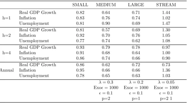
Table 2 reports the results in terms of the Relative RMSE, whereby the benchmark model is the ARDL (1,0). It is defined in the following way:

Relative RM SE_iSize,λ,Exo,,p_;_h =RM SE

Size,λ,Exo,,p i;h

RM SE_iARDL_;_h (1,0)

(5)

Table 2: Relative RMSEs at different projection horizons

SMALL MEDIUM LARGE STREAM

Real GDP Growth 0.82 0.64 0.71 1.44 h=1 Inflation 0.83 0.76 0.74 1.02 Unemployment 0.81 0.90 0.69 1.47 Real GDP Growth 0.81 0.57 0.69 1.30 h=2 Inflation 0.92 0.70 0.76 1.05 Unemployment 0.77 0.74 0.62 1.08 Real GDP Growth 0.93 0.79 0.78 0.97 h=4 Inflation 0.91 0.68 0.64 1.00 Unemployment 0.86 0.74 0.66 0.90 Real GDP Growth 0.86 0.62 0.72 0.73 Annual Inflation 0.95 0.66 0.66 1.36 Unemployment 0.78 0.65 0.63 1.03 λ= 0.3 λ= 0.2 λ= 0.05 Exo= 1000 Exo= 1000 Exo= 1000

= 0.1 = 0.1 = 0.1

p=2 p=1 p=2 1

Table 2 shows that the BVAR specifications outperform the ARDL at each forecast horizon, as they produce lower forecast errors. Moreover, the medium BVAR outperforms the small BVAR at each 13_{A major advantage of the BVAR framework is that it is also able to produce density forecasts besides median projections.} In appendix C (based on Alessandri and Mumtaz, 2017) and D we test the density forecast performance of the three BVARs and produce a density projection for the period 2017-2019. STREAM does not allow us to perform a similar exercise, and hence a density forecast comparison could not be produced.

(12)

projection horizon and for all three variables of interest. On the other hand, there are no improvements to the forecast performance with the larger BVAR as the latter generally performs worse than or as well as the medium BVAR. This is similar to the results obtained by Banbura et al. (2010) who found that for macroeconomic forecasting, a medium-sized BVAR is sufficient for good forecast performance.

3.3 Forecast Comparison

3.3.1 GDP growth

The forecast evaluation period we look at in this exercise is particularly interesting, since Malta registered record GDP growth. Borg et al. (2017) showed that forecast errors committed by the CBM for the period 2013-2015 were quite substantially negative for GDP growth, meaning that CBM forecasts consistently under-predicted GDP growth. Similarly, this forecast evaluation shows that all the models presented here would have on average also under-predicted real GDP growth for the period under consideration.

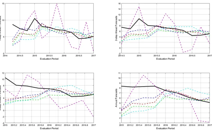
Figure 1: GDP forecast evaluation at different projection horizons

(percentage changes)

Source: Authors’ calculations

Figure 1 shows that all the models find it very difficult to project the extraordinary growth in 2014 and 2015. The BVAR specifications under-predict GDP growth in 2014 and 2015 at each projection horizon,

(13)

and do rather well in 2016. On the other hand, the pattern in STREAM was less stable. Although in general it under-predicted GDP growth when considering the full evaluation period, it under-predicted GDP growth in 2014, over-predicted GDP growth in 2015, and under-predicted 2016.

Indeed, STREAM projections are much more volatile for quarterly projections when compared with the three BVARs. When compared to the ARDL benchmark, STREAM fairs worse in the one-step and two-step ahead horizons, and only marginally better for the four-step ahead horizon. On the other hand, all three BVAR specifications perform better than the ARDL at each forecast horizon, and hence they outperform STREAM. The small BVAR under-performs when compared to the medium and large BVAR at each projection horizon, implying that forecast performance is positively correlated to the cross-sectional size. Nevertheless, the large BVAR under-performs the medium BVAR for the two and four-step ahead horizons, a result similar to the Banbura et al. (2010) finding that a medium-scale BVAR is sufficient for satisfactory forecast performance.

The annual projections smooth out the volatility in the STREAM projections. The latter has been constructed to provide reliable annual projections rather than quarterly projections, and hence, this result is as expected. When smoothing out the inherent quarterly volatility in STREAM, this model performs much better than the ARDL benchmark. In addition, it outperforms the small BVAR and does almost as well as the large BVAR. The only BVAR specification that outperforms STREAM is the medium BVAR, which performs rather well at each projection horizon.

In general, the forecast performance of STREAM seems to improve at longer projection horizons, while the BVAR forecast performance marginally deteriorates, especially at the four-step ahead. Hence, the BVAR might be more useful in providing stable short-run projections rather than a longer run path for real GDP growth. That said however, the short sample size constrained our ability to obtain the optimal priors for the BVAR specifications. Indeed, we set the prior to minimise the sum of RMSE for the one-step ahead on the pre-evaluation period. The results might have changed significantly if we could have searched for optimal priors for the two-step and four-step ahead horizons.

3.3.2 GDP deflator growth

The results obtained for the GDP deflator must also be analysed within the context of the evaluation period utilised in this study. Despite the historically high GDP growth, inflation growth was either below or in line with its historical average. This implies that the Maltese economy went through large structural changes, which are difficult to predict. Indeed, figure 2 shows that all model projections would have on average over-predicted growth in prices during the full evaluation period.

(14)

Figure 2: GDP deflator forecast evaluation at different projection horizons

(percentage changes)

Similar to the results obtained for GDP, STREAM quarterly projections are relatively volatile, while those for the BVAR specifications are more stable. STREAM does as well as the ARDL benchmark at each projection horizon, but under performs substantially in annual terms. On the other hand, all the BVAR specifications improve the forecast performance considerably when compared with both the benchmark ARDL and STREAM.

Moreover, gains are made as the cross-sectional size of the information set gets larger. The medium BVAR outperforms the small BVAR in both quarterly and annual terms. The large BVAR does only marginally better than the medium BVAR in some of the projection horizons, but on average does as well as the medium BVAR for annual projections. Hence, similar to the findings for real GDP growth projections, a medium-scale BVAR already gives a satisfactory forecast performance.

3.3.3 Unemployment rate

In the period 2014-2016, the unemployment rate in Malta followed a downward trend, reflecting the above average growth in economic activity. In general, all model specifications on average over predict the unemployment rate, which is consistent with the under-prediction of real GDP growth and the

(15)

over-prediction of inflation. In addition, the over-over-prediction becomes even larger across all model specifications as the projection horizon increases. These results continue to indicate that the Maltese economy went through a period of structural change in the forecast evaluation period under consideration, which makes forecasting quite challenging.

Figure 3: Unemployment rate forecast evaluation at different projection horizons

(levels)

STREAM does not perform satisfactorily with regards to the unemployment rate when compared with the benchmark model. Indeed, it does either as well as or worse than the benchmark ARDL. On the other hand, despite the challenging forecast environment, the BVAR specifications improve the forecast performance of the unemployment considerably when compared with both STREAM and the benchmark model.

In addition, the forecast performance tends to improve as more and more variables are added to the VAR. Similar to previous findings for both GDP growth and the GDP deflator, the medium BVAR outperforms the small BVAR at any projection horizon. In addition, the large BVAR also outperforms the medium BVAR at each projection horizon, but the gains are much lower than when compared with the small BVAR.

(16)

4 Conclusion

STREAM is a traditional macro-econometric model of the Maltese economy developed at the CBM in part to be utilised for projections. However, its forecast ability had never been tested. Hence, in this paper, we develop an alternative model but with a consistent information set, in order to assess STREAM’s forecast performance of three main macro variables for the period 2014 to 2016.

The alternative modelling framework utilised in this paper was a Bayesian VAR approach similar to Banbura et al. (2010). This setup provides an ideal benchmark for a number of reasons. Firstly, VAR framework is an agnostic data-driven approach that provides an excellent contrast to the economic-theory structural identification in STREAM. And secondly, the Bayesian estimation approach allows us to deal with the curse of dimensionality with ease. Indeed, the dummy-observation prior implementation along with Bayesian shrinkage allows us to include as much information as STREAM.

The BVAR developed here is a BVAR-X, that is, we include both an endogenous and exogenous block. The latter is particularly important for the Maltese economy due to its small open economy structure. Since Banbura et al. (2010) show some evidence that the inclusion of more and more information generally improves forecast performance, we develop three alternative BVARs that differ only with respect to size. The endogenous block in the small BVAR includes only the three main variables of interest, that is, real GDP growth, GDP deflator growth, and the unemployment rate. The medium BVAR increases the endogenous block to 17 variables, and the large BVAR includes 33 endogenous variables.

In order to compare STREAM projections with those obtained from the BVAR, we further benchmark both models against an even simpler ARDL (1,0) modelling framework and compute relative RMSEs with respect to the latter for each specification of the BVAR and STREAM. Results are mixed. Each BVAR specification outperforms the benchmark ARDL and the quarterly projections in STREAM. Indeed, STREAM performs rather poorly with regards to quarterly projections, a result primarily driven by excessive volatility in its quarterly projections. Nevertheless, STREAM performs slightly better with regard to annual projections. Indeed, when focusing on real GDP growth, it is only outperformed by the medium BVAR. On the other hand, each BVAR specification outperforms STREAM at each projection horizon for both the GDP deflator and the unemployment rate.

These results have to be analysed with caution. Firstly, the pre-evaluation sample period to obtain the priors for the BVAR specifications was relatively small, and considered only the one-step ahead projection horizon. A longer pre-evaluation period might have yielded different results. Moreover, the out-of-sample exercise in this paper is not done in real-time, and hence, we do not consider the impact that data revisions might have had on the forecasting properties of the models. Since data revisions in

(17)

Maltese data are frequent and substantial, our results should be treated with caution.

In addition, the constant in each equation in the BVAR was shrunk to zero, a custom utilised in most of the literature. This however may have biased the results since GDP growth is in equilibrium much higher than zero. Indeed, the BVARs developed here seem to be more useful in providing short-term projections rather than long-run projections.

Another limitation is that the forecast evaluation period is a very particular time in the Maltese economy. The structural economic changes that took place in the last few years meant that Malta underwent a period of above average growth, with relatively low inflation rates, and a strong decline in unemployment. For example, Micallef and Ellul (2017) show that potential output has more than doubled when comparing the pre-crisis levels to 2014 and 2015, and project above average growth rates in potential to persist in the long-term. Moreover, Grech and Rapa (2017) document the shift from persistent current account deficits to surpluses, driven primarily by a structural shift in the Maltese economy. Given these structural changes, forecasting has been very challenging, and indeed Borg et al. (2017) show that substantial negative forecast errors have been made by the CBM over the last few years. Indeed, the results obtained in this paper generally show that each model specification would have under-predicted GDP growth, and over-predicted inflation and unemployment.

The BVARs developed in this paper offer not just an opportunity to benchmark the forecast performance of STREAM, but it also adds another modelling framework to the CBM’s forecast toolkit. For example, Leiva-Leon (2017) developed a suite of Structural BVAR and compared median projections from the suite of models to the Banca de Espa˜na macroeconomic projections. Hence, the models developed in this paper can be employed to provide additional modelling information to the forecaster that makes the forecast more robust.

Future work will focus on developing a structural identification to the BVARs developed in this paper. This would primarily produce a historical decomposition of structural shocks that occurred in the Mal-tese economy, such as aggregate demand and aggregate supply shocks. Moreover, the same structural identification would be useful in a projection exercise, as it would be able to recover the implied structural shocks over the projection horizon, which would in turn serve as a useful input to the forecast story.

(18)

References

Alessandri, Piergiorgio and Haroon Mumtaz (2017), “Financial conditions and density forecasts for US output and inflation.”Review of Economic Dynamics, 24, 66–78.

Banbura, Marta, Domenico Giannone, and Lucrezia Reichlin (2010), “Large Bayesian vector auto re-gressions.”Journal of Applied Econometrics, 25, 71–92.

Bloor, Chris and Troy Matheson (2009), “Real-time conditional forecasts with Bayesian VARs: An application to New Zealand.” Reserve Bank of New Zealand Discussion Paper Series DP2009/02, Reserve Bank of New Zealand.

Borg, Ian, John Farrugia, and Reuben Ellul (2017), “Macroeconomic and Fiscal Projections at the Central Bank of Malta.”Quarterly Review, 1, 32–41.

Carriero, Andrea, Todd Clark, and Massimiliano Marcellino (2011), “Bayesian VARs: Specification Choices and Forecast Accuracy.” CEPR Discussion Papers 8273, C.E.P.R. Discussion Papers. Domit, Slvia, Francesca Monti, and Andrej Sokol (2016), “A Bayesian VAR benchmark for COMPASS.”

Bank of England working papers 583, Bank of England.

Giannone, Domenico, Michle Lenza, and Giorgio E. Primiceri (2012), “Prior Selection for Vector Au-toregressions.” Working Papers ECARES 2012-002, ULB – Universite Libre de Bruxelles.

Grech, Aaron G. and Noel Rapa (2017), “An evaluation of recent shifts in Maltas current account position.” InChallenges and opportunities of sustainable economic growth: the case of Malta(Aaron G. Grech and Sandra Zerafa, eds.), 49–60, Central Bank of Malta.

Grech, Owen, Brian Micallef, and Noel Rapa (2014), “A Structural Macro-Econometric Model of the Maltese Economy.”CBM Working Paper Series, version 2.0.

Grech, Owen, Brian Micallef, Noel Rapa, Aaron G. Grech, and William Gatt (2013), “A Structural Macro-Econometric Model of the Maltese Economy.”CBM Working Paper Series, WP/02/2013, ver-sion 2.0.

Grech, Owen and Noel Rapa (2016), “STREAM: A Structural Macro-Econometric Model of the Maltese Economy.”CBM Working Paper Series, WP/01/2016, version 3.0.

G¨urkaynak, Refet S., Burin Kisacikoglu, and Barbara Rossi (2013), “Do DSGE Models Forecast More Accurately Out-of-Sample than VAR Models?” CEPR Discussion Papers 9576, C.E.P.R. Discussion Papers.

Hubrich, Kirstin and Tohmas Karlsson (2010), “Trade consistency in the context of the Eurosystem projection exercises an overview.” Occasional Paper Series 108, European Central Bank.

(19)

Leiva-Leon, Danilo (2017), “Monitoring the Spanish Economy through the Lenses of Structural Bayesian VARs.” Occasional Papers 1706, Banco de Espa˜na.

Micallef, Brian and Reuben Ellul (2017), “Medium-term estimates of potential output growth in Malta.” InChallenges and opportunities of sustainable economic growth: the case of Malta (Aaron G. Grech and Sandra Zerafa, eds.), 15–28, Central Bank of Malta.

Rey, H´el`ene (2016), “International Channels of Transmission of Monetary Policy and the Mundellian Trilemma.” NBER Working Papers 21852, National Bureau of Economic Research, Inc.

Robertson, John C. and Ellis W. Tallman (1999), “Vector autoregressions: forecasting and reality.” Economic Review, 4–18.

Sims, Christopher A and Tao Zha (1998), “Bayesian Methods for Dynamic Multivariate Models.” Inter-national Economic Review, 39, 949–968.

(20)

Appendix A

A.1 Prior implementation and estimation

The prior beliefs are implemented by adding dummy observations in a similar way to Banbura et al. (2010). Before outlining how the prior beliefs are implemented, let us rewrite the modelY =XB+ZG+ in a more compact form:

Y =W C+ (6)

whereY is an n x 1 vector of endogenous domestic variables andW is a (np+1+k)x1 matrix containing lagged valued of the endogenous variables as well as the current values of the exogenous ones (including a column of ones for the estimation of the intercept), i.e. W = (X, Z). C is a (np+ 1 +k)x nmatrix containing all the VAR coefficients and, finally, is anx1 vector of reduced form residual terms which are supposed to be i.i.d. with mean 0 and covariance matrix Σ.

As shown in Banbura et al. (2010), addingTd dummy observationsYdandWd to the VAR is equivalent

to imposing the Normal Inverted Wishart prior which takes the form:

vec(C)|ψ∼N(vec(C0), ψ⊗Ω0)and ψ∼IW(S0, α0) (7)

whereC0= (Wd0Wd)−1Wd0Yd,ψis a diagonal matrix containing the AR(1) variances of the endogeneous

variables, i.e. ψ = diag(σ₁2, . . . , σ_n2), Ω0 = (Wd0Wd)−1, S0 = (Yd−WdC0)0(Yd−WdC0) and α0 =

(21)

DefiningJp=diag(1,2, , p), the dummy observations are added according to the following scheme: Yd=                  diag(δ1σ1,· · ·, δnσn)/λ 0n(p−1)xn . . . . diag(σ1,· · · , σ1) . . . . 01xn . . . . diag(δ1µ1,· · ·, δnµn)/τ . . . . 0kxn                  ; Wd=                    Jp⊗diag(σ1,· · ·, σn)/λ 0npx1 0nxk . . . . 0nxnp 0nx1 0nxk . . . . 01xnp 0nxk . . . . (1 2. . . p)⊗diag(δ1µ1,· · ·, µ1σ1)/τ 0nx1 0nxk . . . . 0kxnp 0kx1 diagk(Exo) | {z } Xd | {z } Zd                    (8)

The first block imposes the prior belief that the endogenous variables follow an AR(1) process. As such, δ1. . . , δn represent the 1st order autoregressive coefficients. As is typical in Bayesian literature, such

belief is weighed by the AR(1) residuals. The degree of tightness is governed by λ. The second block represents the prior belief on the variance covariance matrix being diagonal and containing the AR(1) variances of the endogenous variables. The third sets, i.e. the degree of shrinkage of the constant term to zero. The fourth imposes the sum-of-coefficients prior. As such,µ1. . . , µn represent the mean values

of the endogenous variables. As for the tightness of this prior we follow common practise and set it loosely by imposingτ= 10λ. Finally, the last block governs Exowhich represents the shrinkage to zero of the parameters contained in the matrixG, i.e. the impact of a change in the exogenous variables on the endogenous ones.

Once the dummy variables are appended to the actual data, the system assumes the following form:

Y∗=W∗C+∗ (9)

where Y∗ = (Y0, Yd0)0, W∗= (W0, Wd0) and ∗ = (0, 0d)0.Define alsoT∗=T +Td. As clearly outlined in

Banbura et al. (2010), in order to insure the existence of the prior expectation of ψ it is necessary to include an improper priorψ∼|ψ|−(n+3)/2_{. If this is the case, the posterior takes the following form:}

vec(C)|ψ, Y ∼N(vec( ˜C), ψ⊗(W_∗0W∗)−1)and ψ|Y ∼IW( ˜Σ, T∗+ 2−(np+ 1 +k)) (10)

where ˜C = (W_∗0W∗)−1W∗0Y∗ and ˜Σ = (Y∗−W∗C∗)0(Y∗−W∗C˜). As such, the posterior expectation of

(22)

A.2 Gibbs sampling algorithm details

Consider the model again in the following formY =XB+ZG+and defineβ=vec(B) andγ=vec(G). Moreover, define X∗ = (X0, Xd0),Z∗ = (Z0, Zd0) and ˜C= ( ˜B; ˜G) where ˜B and ˜Gare the OLS estimates

ofY∗ respectively onX∗ andZ∗.

The Gibbs Sampling routine starts by setting reps=1. Moreover, define REPS as the total number of draws.

1. Draw p(β |γ, ψ) from the posterior distributionN(vec( ˜B), ψ⊗(X_∗0X∗)−1. If the candidate draw

is stable keep it, otherwise discard it.

2. Drawp(γ|β, ψ) from the posterior distributionN(vec( ˜G), ψ⊗(Z_∗0Z∗)−1

3. Drawp(ψ|β, γ) from the posterior distributionIW( ˜Σ, T∗+ 2−(np+ 1 +k))

Repeat steps 1, 2 and 3 forreps= 1, . . . , REP S.

A.3 Estimation setup

The Gibbs Sampling routine is run by setting REPS=15000. The posterior distributions of the relevant parameters are simulated, and used for forecasting purposes, by discarding the first 10000 repetitions in order to minimise the effect of initial values.

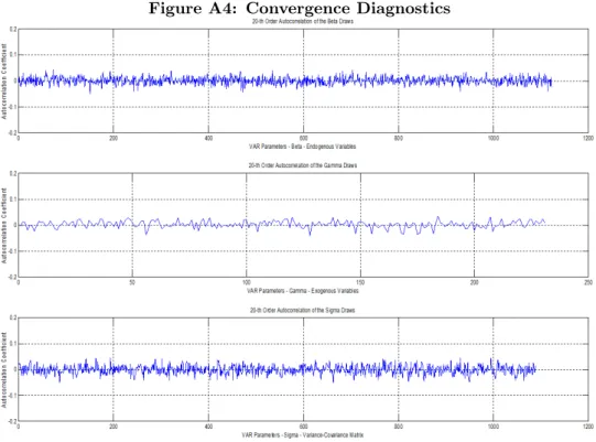
A.4 Convergence diagnostics

This appendix assesses the convergence of the Gibbs Sampling routine. In order to do so, the 20-th order autocorrelations of the retained VAR parameter draws from their respective posterior distributions have been calculated. Figure A.4 shows the results by separating beta, gamma and sigma coefficients according to whether they refer to the impact of lagged endogenous variables, the impact of the exogenous ones and the variance-covariance matrix. On the horizontal axis the VAR parameters have been aligned while on the vertical axis the 20-th order autocorrelation coefficient of their draws is shown.

The autocorrelation coefficients are safely below 0.2 and in most of the cases very close to zero. This suggests that the model has converged as the draws are almost independent.

(23)

Figure A4: Convergence Diagnostics

(24)

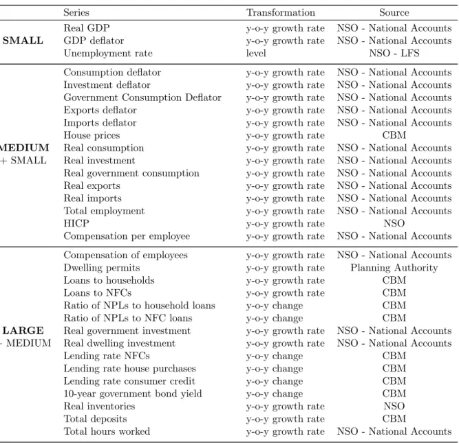
Appendix B - Data

Table B.1 outlines the endogenous variables utilised for this study. The first block describes the trans-formation and sources related to the SMALL BVAR. The second block reports the additional variables related to the MEDIUM BVAR, and the final block reports the additional variables related to the LARGE BVAR.

Table B.1: Endogenous variables

Series Transformation Source

Real GDP y-o-y growth rate NSO - National Accounts

SMALL GDP deflator y-o-y growth rate NSO - National Accounts

Unemployment rate level NSO - LFS

Consumption deflator y-o-y growth rate NSO - National Accounts Investment deflator y-o-y growth rate NSO - National Accounts Government Consumption Deflator y-o-y growth rate NSO - National Accounts Exports deflator y-o-y growth rate NSO - National Accounts Imports deflator y-o-y growth rate NSO - National Accounts

House prices y-o-y growth rate CBM

MEDIUM Real consumption y-o-y growth rate NSO - National Accounts

+ SMALL Real investment y-o-y growth rate NSO - National Accounts

Real government consumption y-o-y growth rate NSO - National Accounts

Real exports y-o-y growth rate NSO - National Accounts

Real imports y-o-y growth rate NSO - National Accounts

Total employment y-o-y growth rate NSO - National Accounts

HICP y-o-y growth rate NSO

Compensation per employee y-o-y growth rate NSO - National Accounts Compensation of employees y-o-y growth rate NSO - National Accounts

Dwelling permits y-o-y growth rate Planning Authority

Loans to households y-o-y growth rate CBM

Loans to NFCs y-o-y growth rate CBM

Ratio of NPLs to household loans y-o-y change CBM

Ratio of NPLs to NFC loans y-o-y change CBM

LARGE Real government investment y-o-y growth rate NSO - National Accounts + MEDIUM Real dwelling investment y-o-y growth rate NSO - National Accounts

Lending rate NFCs y-o-y change CBM

Lending rate house purchases y-o-y change CBM

Lending rate consumer credit y-o-y change CBM

10-year government bond yield y-o-y change CBM

Real inventories y-o-y growth rate NSO

Total deposits y-o-y growth rate CBM

(25)

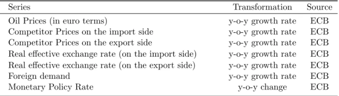
Table B.2 reports the exogeneous variables utilised in this study. Each BVAR takes the same exogeneous variables, which control for foreign demand, inflation, and the exchange rate.

Table B.2: Exogeneous variables

Series Transformation Source

Oil Prices (in euro terms) y-o-y growth rate ECB

Competitor Prices on the import side y-o-y growth rate ECB Competitor Prices on the export side y-o-y growth rate ECB Real effective exchange rate (on the import side) y-o-y growth rate ECB Real effective exchange rate (on the export side) y-o-y growth rate ECB

Foreign demand y-o-y growth rate ECB

(26)

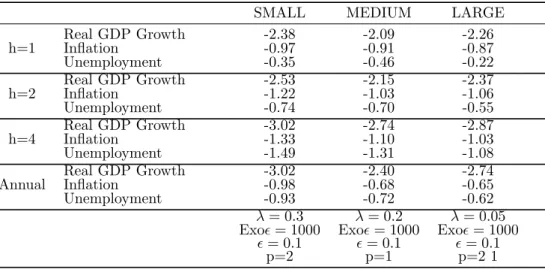
Appendix C - Density forecast performance

This appendix assesses the density forecast performance of each of the three BVARs considered. The way such a performance is evaluated is through a scoring rule which is a loss function that takes the density forecast and the actual outcome as its arguments. Following Alessandri and Mumtaz (2017) here a logarithmic scoring rule is used. To be more precise, for each variableyi at each forecast horizon h,

the logarithmic scores are calculated as follows:

LSSize,λ,Exo,,p_i_;_h = 1 T1−T0−h+ 1 T1−h X t=T0 lnf_iSize,λ,Exo,,p_;_t₊_h_|_t (yi;t+h) (11)

wheref_iSize,λ,Exo,,p_;_t₊_h_|_t (.) represents the density forecast of variableyi at forecast horizon h whiley(i;t+h)

represents the observed value. Size, λ, Exo, , p are defined as in section 2.4. The logarithmic scores take high values if the forecast densities assign a high probability to the actual outturn. The results are reported in Table C.1.

Table C.1: Density forecast performance

SMALL MEDIUM LARGE

Real GDP Growth -2.38 -2.09 -2.26 h=1 Inflation -0.97 -0.91 -0.87 Unemployment -0.35 -0.46 -0.22 Real GDP Growth -2.53 -2.15 -2.37 h=2 Inflation -1.22 -1.03 -1.06 Unemployment -0.74 -0.70 -0.55 Real GDP Growth -3.02 -2.74 -2.87 h=4 Inflation -1.33 -1.10 -1.03 Unemployment -1.49 -1.31 -1.08 Real GDP Growth -3.02 -2.40 -2.74 Annual Inflation -0.98 -0.68 -0.65 Unemployment -0.93 -0.72 -0.62 λ= 0.3 λ= 0.2 λ= 0.05 Exo= 1000 Exo= 1000 Exo= 1000

= 0.1 = 0.1 = 0.1

p=2 p=1 p=2 1

Overall, the logarithmic scores confirm that the density forecasts tend to be more accurate as the BVAR size gets larger. This, together with the results shown in Section 3.2, would further confirm how including more information in the model helps improve the forecast power.

(27)

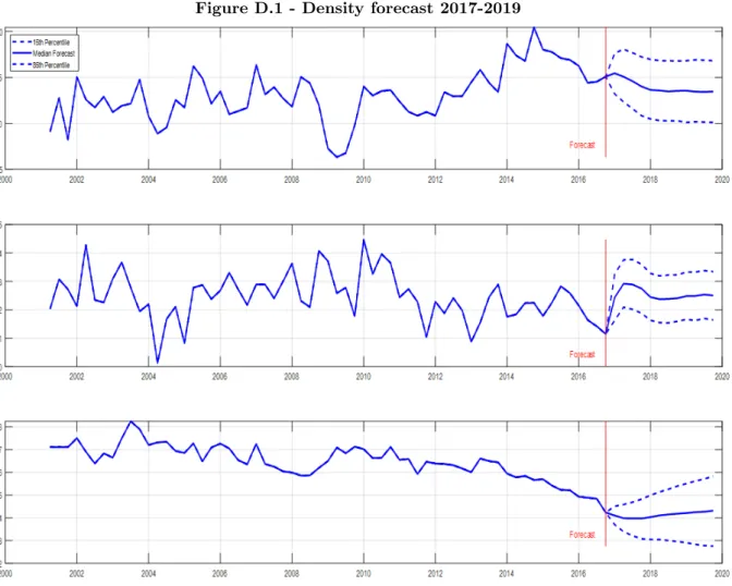
Appendix D - Density forecast over 2017-2019

This appendix shows how one of the outcomes automatically provided by the Bayesian approach is the possibility to get forecast distributions for the variables of interest. In this particular case, figure D.1 shows the median forecast together with the 15th and 85th percentiles relative to GDP growth, GDP deflator growth and unemployment rate. The forecasts are obtained by estimating the Large BVAR described in section 2 by using data from 2001Q1 till 2016Q4. The projections are relative to the 2017Q1-2019Q4 period. The priors used in this estimation are the same as those used in section 3.2 for the same BVAR.

Figure D.1 - Density forecast 2017-2019

Compared to the release NSO 041/2017, median projections for 2017 of GDP growth came out lower than outcomes, while median projections for the growth in the GDP deflator were higher. Moreover, the median projections for the unemployment rate were broadly in line with outcomes. For all three variables however, outcomes were well within the density forecast bands.