RESEARCH ARTICLE
The flow around a surface mounted cube: a characterization
by time‑resolved PIV, 3D Shake‑The‑Box and LBM simulation
A. Schröder1 · C. Willert2 · D. Schanz1 · R. Geisler1 · T. Jahn1 · Q. Gallas3 · B. Leclaire4
Received: 19 March 2020 / Revised: 22 June 2020 / Accepted: 13 July 2020 / Published online: 9 August 2020 © The Author(s) 2020
Abstract
The flow around a surface mounted cube with incoming turbulent or laminar boundary layer has been topic of many experi-mental and numerical investigations in the past decades. Despite its simple geometry the flow generates a set of complex vortical structures in front and around the cube, includes flow separation at the three front plane edges with corresponding subsequent shear layer dynamics enveloping recirculation zones. Downstream of the cube a large unsteady flow separation region is present which is associated with typical quasi-periodic bluff-body wake dynamics. Therefore the flow configura-tion is well suited to enhance the understanding of similar unsteady and separated flow phenomena in many aerodynamic and engineering applications. In the present experimental investigation we aim at resolving a large spectrum of spatial and temporal scales in the flow around a cube with incoming laminar and turbulent boundary layers by using the most recent developments of dense 3D Lagrangian particle tracking (LPT) and high resolution TR-PIV for Reynolds numbers based on cube size in the range ReH=U
∞H𝜈 −1
=2000−8000 . The results documented in the present paper consist of snapshots
and the analysis of long time-series of highly resolved 3D and 2D velocity fields suited to enhance the understanding of coherent structure dynamics and of corresponding statistical Lagrangian and Eulerian flow properties. Premultiplied veloc-ity spectra and 3D pressure distributions are calculated and discussed as well. Finally, the measurement data is compared to results obtained with a simulation based on the lattice Boltzmann method (LBM).
Electronic supplementary material The online version of this article (https ://doi.org/10.1007/s0034 8-020-03014 -5) contains supplementary material, which is available to authorized users. * A. Schröder
[email protected] * C. Willert
1 Deutsches Zentrum für Luft- und Raumfahrt (DLR), Institute
of Aerodynamics and Flow Technology, 37075 Göttingen, Germany
2 Deutsches Zentrum für Luft- und Raumfahrt (DLR), Institute
of Propulsion Technology, 51170 Köln, Germany
3 Univ. Lille, CNRS, ONERA, Arts et Metiers Institute
of Technology, Centrale Lille, UMR 9014, LMFL, Laboratoire de Mécanique des fluides de Lille, Kampé de Fériet, 59000 Lille, France
4 DAAA, ONERA, University Paris Saclay, 92190 Meudon,
Graphic abstract
1 Introduction
In the last few decades, there has been extensive research on turbulent boundary layer (TBL) and turbulent channel flows around wall-attached obstacles, including cubes with various aspect ratios roughly in the range of 𝛿∕H≈ 0.25–5
or H∕h≈ 0.1–0.3. Here, H is the cube or obstacle height, 𝛿
represents the boundary layer thickness and h the channel height. In the first group of investigations, mainly the case with high Reynolds numbers ( Re
H>10, 000 ) and incoming
TBL flows has been addressed (e.g., mimicking buildings in atmospheric BL) with the aim of identifying the gen-eral flow features around the cube. Extensive experimental studies have been performed by Castro and Robins (1977), Martinuzzi and Tropea (1993) and Meinders et al. (1999) primarily focusing on unsteady pressure distributions gained by probe measurements and wall-shear stress visualizations
using oil-film techniques or similar. These studies gained many basic insights into the mean 3D flow structures around and in the wake of the cube using assumptions governed by topological concepts. Hussein and Martinuzzi (1996) generated a detailed velocity vector map in several planes and locations around the cube using one-point LDA meas-urements to investigate the budget balance of the turbulent kinetic energy transport by mean and fluctuation velocity statistics. Near-surface PIV results of the flat plate around and at the walls of the cube itself by Depardon et al. (2005, (2006) have allowed the estimation of the related skin fric-tion vector fields along with the identificafric-tion of locafric-tions of mean separation lines, foci- and saddle-point topologies (Depardon et al. 2007), which previously was restricted to qualitative visualizations only.
On the other hand, extensive numerical simulations using advanced methods like unsteady RANS (Iaccarino
et al. 2003) or large eddy simulation (LES) (Krajnović and Davidson 2002; Lim et al. 2009), the latter combined with experiments) have been performed at relatively high Reyn-olds numbers. Direct numerical simulations (DNS) so far are limited to lower Reynolds numbers (Diaz-Daniel et al.
2017; Yakhot et al. 2006a, b) but enable a complete analysis of the unsteady behavior of 3D coherent flow structures, which in the past could be identified only partly if not even limited to mean flow structures. These structures and their characteristic dynamics depending on the governing condi-tions within the specific flow regions around the cube have been topic of individual research interest. Lim et al. (2007) experimentally investigated Reynolds number effects on the mean and fluctuating velocities and pressures on and around the cube for broad range of Reynolds numbers, including the investigation on a large (6 m) cube in an atmospheric TBL. In a subsequent study Lim et al. (2009) focused their investigations mainly on the flow, shear layers and recircu-lation regions above and along the three streamwise cube surfaces. In the work of Yakhot et al. (2006a), the unsteadi-ness of the vortical structures and induced bimodal verti-cal velocity distribution in front of the cube, which are the midpoints of the well-known horseshoe vortices surrounding the cube in the near wall region, was the main focus of their investigation. The extensive DNS work by Diaz-Daniel et al. (2017) of the flow around a cube, with incoming turbulent and several laminar boundary layer flows at six different low Reynolds numbers, enables the investigation of the specific dynamics of the shear layers, horse-shoe vortices and wake flows through direct comparison. They showed that the laminar in-flow condition features Reynolds num-ber dependent specific wake dynamics with distinct peaks at several Strouhal numbers associated with the interference of transitional shear layers, the stability of the horse-shoe vortex and hair-pin vortices with the overall flow topolo-gies of the separated flow region. This work is the closest numerical research case when compared to the parameters of the present experimental study concerning the choice of flow configurations. Although for the majority of flow cases the DNS was performed at slightly lower Reynolds numbers than in the present experimental investigation, many features quantified by the present flow measurements are very similar and can be compared directly.
In order to augment the recent DNS results with experi-mental data, advanced particle image based velocime-try methods were applied on a cube configuration in the water flow facility THBV1 at ONERA, Lille. The novel
dense Lagrangian particle tracking (LPT) technique Shake-The-Box (STB) (Schanz et al. 2016) with subsequent data assimilation by FlowFit (Gesemann et al. 2016) provided
temporally resolved 3D3C data of the flow topology around the cube. In addition, a high resolution, time-resolved 2D2C (TR-) PIV technique (Willert 2015) provided long time-series of particle image data at selected locations to characterize the in-flow conditions and allow spectral investigations of the flow dynamics. The 3D STB and (with limitations) the TR-PIV techniques, in principle, can be adapted to flows with much higher Reynolds numbers and flow conditions that currently are beyond to reach of DNS. The employed measurement techniques are capable of very high dynamic temporal and spatial range, at least for one-point statistics of the velocity vector data in small fields of view (Beresh et al. 2018) or by multi-pulse STB (Novara et al. 2016, 2019). For example, in compressible and swept wing aerodynamics there is continued research interest in the laminar-transitional flow conditions when the surface mounted obstacle heights H are significantly smaller than the BL thicknesses, thus mimicking surface imperfections and roughness caused by limitations in manufacturing capa-bilities in aerodynamic vehicle production. These surface imperfections, typically in the μm-range, lead to modal and
non-modal growth of the induced disturbances and then to (premature) boundary layer transition during flight. The experimental investigation of transitional flow with grow-ing small-scale disturbances in thin boundary layers around wings at transonic velocities has recently become feasible with micro 3D STB measurement methods (Novara et al.
2019). In this context, the present work can be seen as a preparatory step, taken so as to allow such laminarity studies in future research.
The collected experimental data set is also intended as a reference case for CFD validation, especially for advanced scale resolving simulation methods. In this context the Lat-tice Boltzmann method (LBM) has regained interest within the CFD community during the past decade since it enables time-transient simulations and gives access to instantaneous solutions of the resolved flow field. LBM is known to be capable of accurately simulating detached incompressible turbulent flows, and is therefore well suited for the turbulent flow configuration reported in this paper.
The following section describes the experimental setup of the TR-PIV and 3D STB measurement systems at the THBV water flow facility at ONERA Lille and the related specific calibration and evaluation schemes. The incoming BL flow conditions could be accurately characterized through an upstream TR-PIV measurement. Section 3 provides instan-taneous and mean flow results of the TR-PIV and 3D STB measurements for a selected subset of the investigated cases. A brief description on Reynolds number effects for four lam-inar test cases is provided. In a next step results obtained with LBM are compared with the corresponding experimen-tal flow field data for the turbulent test case. Further post-processing and analysis tools applied to the collected data
are explained and the respective findings are presented and described. The last section provides a summary of the gained results along with a short outlook.
2 Experimental set‑up and tools
2.1 Facility and configurationONERA Lille’s low speed water tunnel (THBV) is a grav-ity-driven, closed-loop water tunnel equipped with very good optical access, therefore making it ideally suited for particle- and laser-based velocimetry techniques. It has a square test-section of 300×300 mm2 and can be operated
at free-stream velocities ranging from 0.1 to 0.9 m/s. For the present test campaign, a splitting plate, with an elliptical leading edge has been placed at mid span so as to generate a boundary layer flow (see Fig. 1). In order to minimize laser light reflections on this plate, a transparent glass insert of
150×150 mm2 , centered in span, is placed at the streamwise
position targeted for the TR-PIV and 3D STB measurements. The cube of height H=10 mm, also made of glass, is fixed
on this plate with a refractive index matched glue and is located at a streamwise distance of 510 mm from the leading edge of the plate. On the premise of having a refractive index closer to that of water, different materials for the manufac-ture of the cube were investigated in a preliminary study,
such as hydrogel based on polymerized acrylamide and PTFE (polytetrafluoroethylene or Telfon). However, none of the attempts provided a sufficiently rigid cube with defined sharp edges or sufficient transparency (e.g. for PTFE), so that glass was finally chosen. As a consequence, this neces-sitated specific steps in the LPT data processing to account for the refractive index variations along the imaging path as described in Sect. 2.5.
In the tests presented here, both the situations of laminar and turbulent boundary layers at thicknesses comparable to that of the cube height are considered. The TBL is triggered by a 2D step of 1.5 mm height covering the whole span that is inserted into the groove near the leading edge of the plate shown in Fig. 1, such that a low Reynolds number turbulent boundary layer is developing downstream of this tripping device.
2.2 Measurement conditions and coordinate system
For both 2D2C PIV and 3D STB data was acquired for the tripped, turbulent boundary layer case
U
∞=0.8 m/s at Re𝜃=1 000 ) and four laminar BL cases
( U∞=0.2, 0.4, 0.6 and 0.8 m/s respectively
correspond-ing to (rounded) ReH=2000, 4000, 6000 and 8000 with
the cube height H=10 mm and aspect ratios 𝛿∕H as
indi-cated in Table 2. With reference to the Reynolds numbers
estimated by TR-PIV upstream of the cube, we decided to round-up the values for the actual position of the cube for all further descriptions.
The coordinate system used throughout the paper is defined as follows: the plane onto which the cube is mounted is spanned by the x-axis, aligned in streamwise direction, and the z-axis in spanwise direction. Accordingly, the y-axis defines the wall-normal direction. The origin of the coordi-nate system is assigned to the base of the back face of the cube at mid-point of the spanwise dimension z (see also Fig. 2b). Were appropriate length dimensions are normalized by the cube dimension H=10 mm.
2.3 Time‑resolved 2D‑2C PIV
The following provides an overview of the high resolution 2D-2C PIV measurements obtained along the center plane (symmetry plane, z=0 ) both upstream and around the
cube. Measurements were performed at four locations as shown in Fig. 3. The upstream position (Pos.1) was chosen
to characterize the inflow boundary layer profile upstream of the cube at x= −52 mm ( x∕H= −5.2 ). Position 3 was
centered at x=15 mm downstream of the cube and captured
the mean flow reattachment point in the wake of the cube. Position 2 mapped the area above the cube, while Position 4 sampled the stagnation zone directly upstream of the cube.
The PIV measurement approach employed in these exper-iments closely follows the procedures and methods laid out in the paper by Willert (2015). The near-wall measurement approach has been successfully used in a variety of previous applications, such as for turbulent boundary layer measure-ments with zero and adverse pressure gradients (Cuvier et al.
2017; Willert et al. 2018). The imaging setup was designed for a magnification of m=0.66 using a macroscopic lens of
100 mm focal length (Zeiss-Planar T100/2) at an aperture of f-number 4.0. On the imaging side a high-speed cam-era with a 4 megapixel CMOS sensor was used (PCO AG, DIMAX-S4), which has a pixel pitch of 11μ m
correspond-ing to 16.67μm/pixel in object space (see Fig. 2 with the
set-up at THBV). Using macroscopic imaging the small-est viscous scales anticipated for the turbulent case of the test matrix, corresponding to U
∞≈0.8 m/s with Re𝜏 =400
and Re
𝜃 =1000 amounted to about 28μ m per viscous unit
( y+
= 𝜈∕u𝜏 ) and could be resolved with nearly single pixel
resolution.
For the upstream boundary layer measurements the field of view of the camera was reduced to 240 pixel width and 1008 pixel in height ( 4.0×16.7 mm2 ). This reduction
allowed an increase of the number of acquired images to more than 100,000 during a single run. The other roughly 5–10 mm wide measurement areas were illuminated by a
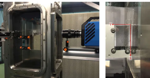
Fig. 2 High-resolution 2D-2C TR-PIV setup to image the upstream area of the cube. The calibration target can be seen installed upstream of the
cube (a) and calibration target placed downstream of the cube (b). The mean flow direction in the test section is downward, along X
Fig. 3 TR-PIV measurement locations. Red lines indicate sample locations for spectral estimates and velocity profiles
pair of externally modulated continuous wave lasers (Kvant Laser, SK) with a combined output power of nearly 10 W at a wavelength of 520 nm. Focusing lenses narrowed the light sheet to a thickness of about 200–300 μ m in the
measure-ment area. Synchronization between modulated laser and high-speed camera was provided through a separate multi-channel pulse generator (Arduino MEGA 2560).
The acquired TR-PIV image sequences were processed using a 2D-2C PIV processing algorithm based on cross-cor-relation, using a coarse-to-fine pyramid approach with image deformation and intermediate validation (normalized median filter and smoothing). To achieve optimal, noise-minimized velocity estimates, a pyramid correlation scheme, similar to the algorithm proposed by Lynch and Scarano (2013), was employed and used up to five consecutive frames. For the upstream measurement position (Pos.1 in Fig. 3) a large aspect ratio of 64×3 pixels ( 1070×50μm2 ) was chosen to
achieve optimal wall-normal spatial resolution in the recov-ered velocity profiles. In wall-normal distance the sampling distance was fixed at 1 pixel ( 16.7,μm . The data from all
other measurement locations (Pos.2, 3 and 4) were processed with a final interrogation window size of 16×16 pixels
( 270×270μm2 ). Sampling distances were approximately
30% of the sample size.
2.4 3D STB experimental set‑up
The flow around the cube was also investigated with the time-resolved 3D STB technique enabling dense Lagrangian particle tracking in an extended volume around the cube. In total seven high-speed cameras and a high repetition laser for volume illumination (see Figs. 4 and 5) were used to carry out the experiments. Measurements were performed at the same in-flow conditions as for the TR-PIV measurements reported in Sect. 2.3. Corresponding acquisition parameters for each point of the test matrix are given in Table 1. Both flow cases are of eminent interest for the understanding of this complex geometry induced flow separation case with transitional and turbulent shear and wake flow development regions.
A hexagonal prism was installed at the front glass win-dow of the water tunnel to realize nearly orthogonal viewing conditions through the air-glass-water interfaces for each camera avoiding strong astigmatism effects for particle imaging. In order to capture the flow in the measurement volume around the cube in full time-resolution, a system of seven high-speed cameras ( 6× PCO.Dimax S4 with 4 MP
with 11μ m pixels and 1× Phantom Miro 340 with 10μ m
pixels reduced to ≈2 MP) was set up. The six PCO cameras
obliquely viewed the prism with nearly the same relative viewing angles through the prism, which itself was attached to the glass window of the water tunnel with a glycerol-water
Table 1 Measurement matrix
for the volumetric 3D STB experiment
Condition Laminar Turbulent
Tunnel setting, U∞ [m/s] 0.8 0.6 0.4 0.2 0.8 Acquisition rate [Hz] 1500 1125 750 375 1500 Total image count 29,400 22,050 22,044 22,044 55,125
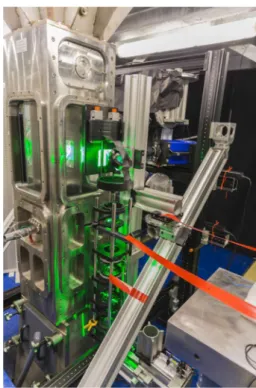
Fig. 4 Laser volume illumination of particles in the flow around the surface mounted glass cube as viewed through six-folded prism (a). Six high-speed cameras pointed at the measurement volume (b). A seventh camera viewed the cube from the opposite side
Fig. 5 Photograph of the experimental setup with light-sheet optics attached to the tunnel and camera system in the back
mixture as a thin adhesive fluid layer in between the two parallel glass surfaces of the prism and water tunnel, respec-tively. The seventh camera (Phantom Miro) viewed through the window on the opposite side and was set to a high-magnification factor to image only the area surrounding the cube. This camera acquired complementary images of the “shadow” regions induced by refraction through the cube on the images of the other six cameras. A high-repetition laser system (Quantronix Darwin Duo) with an energy of 20 mJ per pulse at 1 kHz was used to illuminate a rectangular sec-tion of approximately 80 mm in streamwise direcsec-tion and 20 mm in wall-normal direction using beam shaping optics and a passe-partout to cut off the weaker intensity of the expanded laser beam. In addition the collimated laser beam was back-reflected through the measurement volume by a mirror (see Figs. 4 and 5). The common field of view of the six camera system covered a section of approximately 70 mm in spanwise direction. The six PCO cameras were equipped with 100 mm focal length lenses (Zeiss Makro-Planar T 100/2) while the Phantom camera was equipped with a 200 mm lens (Nikon Micro Nikkor 200/4).
2.5 Challenges in STB particle tracking around the cube
For the specific challenges faced during the calibration of the 3D STB system and subsequent evaluation of particle images several improvements on top of the existing time-resolved Lagrangian particle tracking code have been implemented and tested. First the calibration and volume matching of the seventh camera view with a much smaller field of view and higher magnification factor has been adapted. Starting with the calibration target the number of visible markers in the seventh camera was too low in order to realize a common volumetric calibration together with the common view of the other six cameras. Therefore, as first indicator, the eight cube edges were detected manually in the field of view of the seventh camera. As their 3D positions are known, they were used as preliminary 3D–2D point correspondences. This calibration was refined by tracking results that were gained using only the other six cameras: the tracked parti-cles located in the common view with the seventh camera were back-projected into this camera using the preliminary calibration, which was accurate enough to identify the cor-responding peaks in the original camera image. The particle coordinates and the identified corresponding peak locations constitute a huge number of accurate 3D–2D point corre-spondences, allowing for a precise calibration of the seventh camera. Then for all cameras, a local determination of the particles’ optical transfer function (OTF) were estimated according to Schanz et al. (2012), following the volume self calibration step (Wieneke 2008).
In a second challenge, a volumetric mask was created in order to take into account that the cube is located within the measurement volume and thus within the individual cameras lines-of-sight. Although the cube was made of glass (neces-sary for the volumetric, collimated and back-reflected laser illumination), its refractive index ( n=1.520 ) is sufficiently
different from the refractive index of water ( n=1.333 ). Due
to this difference in refractive index the images of particles located in the ‘shadow’ of the cube for a specific camera (the green area in Fig. 6a) will undergo a significant shift, as they are viewed through the cube glass surfaces under different angles. This displacement would corrupt the recon-structed 3D position, therefore the cameras seeing the parti-cle through the cube glass need to be ignored in the shaking process.
Due to the simple geometry of the cube, the projection points of individual particles, combined with a constraint on their height above the wall, can be used to isolate par-ticles that are viewed through the cube for each camera. As a ‘mask’ we will define the image of the top surface of the cube for a given camera (see Fig. 6b for one exemplary camera view). It should be noted that no image process-ing is performed with this mask; it purely defines a search
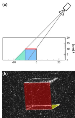
Fig. 6 a Single camera viewing the cube, with indicated ‘shadow’ area (green), where particle images would appear displaced. b Rep-resentative particle image of the cube as viewed by the camera. A 2D mask applied on cube’s top is indicated in red
area. Figure 6a illustrates that particles which are projected onto this mask for a given camera could be located in three domains. Particles located above the cube are visible with-out disturbance by all (Depardon et al. 2006) camera views, therefore all cameras can be used for the shaking procedure. Particles located in the shadow region behind the cube are displaced and have to be excluded from the reconstruc-tion process for the given camera view. A particle could also be (falsely) reconstructed within the cube, however this rarely occurs. In this case the current camera is also ignored. Therefore, the condition whether a given camera view should be included in the shaking process for a given particle is dependent on the particle location [(above the cube ( y>10 mm) or below the cube ( y<10 mm)] and on
its projection point (within the mask or not). Despite leav-ing out multiple cameras in some regions, it was possible to view all areas around the cube with at least four cameras due to the chosen 6+1 camera configuration with one
cam-era viewing the cube orthogonally from the opposite side. Particles below y=10 mm and a projection point within
the yellow area could either be located in front of the cube or in the small shadow region on the side. It was decided to not apply a mask in this region as this would have resulted in some (small) regions being reconstructed by less than four cameras.
The polyamide seeding particles sourced from Vestosint introduced an unfavorably high dynamic range of intensities accompanied by a variation of the particle image diameters between two and eight pixels. The utilized particles have a polydisperse distribution with a large variation of shapes and diameters between ≈5μm and 80μm and an average
diam-eter of ≈30μ m. For future investigations in water
facili-ties similar to the present we plan to use particles that are less polydisperse, such as, for instance, low-cost polyamide particles (e.g., Orgasol). STB evaluation was further com-plicated by the fact that the flow is locally highly turbulent and three-dimensional with very strong shear regions near the geometry-induced flow separations starting at the front edges of the cube. Near the strong shear layers a predictor from neighboring particles was not reliable. Furthermore, particles are subjected to strong acceleration events while passing around the edges of the cube or move within the turbulent wake of the cube which resulted in a reduction in accuracy of their predicted position for the following time step and subsequent loss of some tracks in these regions. In part, this is due to limitations of the temporal resolution.
In addition, high intensities in the background image from the light scattered at the cube edges further complicated the evaluation situation of particle tracks close to the edge posi-tions. To overcome some of the difficulties related to these regions and high acceleration events we used averaged 3D flow field results from preliminary STB evaluations. Results from the evaluation of one run per flow case were binned in
3D bins of 1 mm edge length (akin to the method introduces in Sect. 3.4). The collected 3D velocity averages in each of these small sub-volumes are then used as a predictor field of particle position 𝐩 . The search radius around a point
pre-dicted by this field is then parameterized by the local RMS value determined in the binning process. Depending on the particle location this RMS-value can be very small (e.g., in a region far away from the cube) or quite large (e.g., in the shear layers close to a cube edge). In order not to reject true events, the following relation was used for the RMS-based search radius: 𝜎RMS=7∗RMS+0.5 pixel. The locally
var-ying expression 𝐩+ 𝜎RMS is used throughout the complete
volume both for the identification of new tracks within the clouds of newly reconstructed particles and as an outlier criterion for already tracked particles. On average around 250–400 particles (about 0.8% of the particles) are excluded per time-step by this criterion. These additional schemes were included in the STB evaluation to enable a robust and reliable 3D Lagrangian particle tracking in the full volume.
2.6 FlowFit: Navier–Stokes regularized data assimilation to a Cartesian coordinate system
After fitting the found particle tracks temporally by third-order B-splines with an optimized parametrization from spectral analysis (TrackFit by Gesemann et al. 2016), we gain improved particle positions, velocities and accelerations in a scattered manner within our 3D measurement volume by analytical differentiation. To get the full time-resolved 3D velocity fields and the related velocity, gradient tensor- and pressure fields on (any) Cartesian grid, we further calculate a data assimilation of the scattered particle information using a continuous flow field representation by fitting a system of uniform third order cubic B-splines to the given scat-tered discrete velocity and acceleration vectors gained from the particle tracks. The FlowFit data assimilation scheme applies a fully incompressible Navier–Stokes regularization which is imposed onto the grid of B-splines by optimizing iteratively a set of related cost functions using a non-linear optimization algorithm (here LBFGS). The related cost functions are weighted according to the measurement noise and are penalizing strong curvature, divergence of velocity and of Eulerian acceleration together with the differences between measurements and interpolations at particle loca-tions (Gesemann et al. 2016). FlowFit avoids the classical correlation-window-based low-pass filtering (a common short-coming of tomographic PIV), increases the spatial resolution by following the imposed physical constraints and allows for an arbitrary sampling on desired grids as well for derivations which can be directly computed on any position in the measurement volume from the continuous B-spline functions (e.g., vorticity, strain, Q-criterion and similar quantities).
2.7 LBM methodology
The flow around the cube is simulated using the lattice Boltzmann flow solver ProLB. This solver is based on the lattice Boltzmann method (Qian et al. 1992; Chen and Doolen 1998) that is implemented on a non-uniform octree grid (Touil et al. 2014). Briefly outlined, the LBM is based on a particle collision model in the Lagrangian frame of reference. It can be interpreted as a discrete version of the Boltzmann equations that govern the gas motion, rep-resented at the mesoscopic level by a probability density function of a reduced number of velocity vectors. The LBM is thus a sequence of propagation and collision of fictitious particles. The ability of LBM to simulate bluff body flows at different Reynolds numbers has already been demonstrated by Liu et al. (2008) and Islam et al. (2012). The present simulation is based on ProLB, a novel CFD solver intended to address low-Mach number flows around highly complex geometries. The volume mesh is a multi-resolution Cartesian grid that is generated automatically. Complex solid objects are treated using an immersed solid boundary algorithm. The turbulence modeling is based on a large eddy simula-tion (LES) approach with a shear improved Smagorinsky model. A wall model is added to take into account near-wall turbulence effects and adverse pressure gradients (Tannoury et al. 2014). In this study the flow condition with incoming turbulent boundary layer with U
∞=0.8 m/s is considered.
For the volumetric grid refinement, the ProLB solver requires a Cartesian grid with embedded resolution domains. Special care is given to ensure sufficient distance between two consecutive resolution domains to allow a correct propa-gation of the velocity distribution functions at the nodes. The simulation domain counts a total of seven resolution domains corresponding to 11×106 equivalent fine voxels in
the volume. In terms of initial conditions, a constant veloc-ity profile is set at the inlet of the simulation domain, while a pressure release boundary condition is used at the outlet. A no-slip boundary condition is set on all the walls (flat
plate, cube, tunnel walls) and the floor of the flat plate is treated with an artificial roughness to ensure a proper devel-opment of the incoming turbulent boundary layer. The inlet velocity profile has been adjusted accordingly to match the experimental velocity profile, both in magnitude and fluctua-tions, that is captured upstream of the cube at x= −52.0 mm
( x∕H= −5.2 ). The convergence is monitored using probes
located near the inlet and upstream and downstream the cube. The fluid measurement files are averaged over the last 200,000 iterations, corresponding to an average over 57.7 s physical time. A typical time-averaged flow field is provided in Fig. 7. It exhibits the flow structures that are discussed in the next section in comparison to the experimental results.
Fig. 7 Mean flow field around the cube from the LBM simulation for the turbulent test case at U∞=0.8 m/s
(a)
(b)
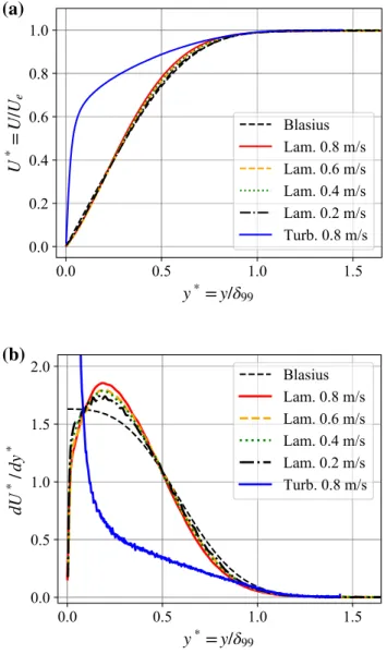
Fig. 8 a Mean velocity profiles at x= −52 mm upstream of the cube scaled with outer velocity Ue and boundary layer thickness 𝛿99 . b
Pro-files of the mean normalized velocity gradient dU∗ ∕dy∗
3 Results and discussion
3.1 Characterization of the upstream flow
As described in Sect. 2.3, the flow conditions upstream of the cube were characterized using 2D-2C TR-PIV sequences acquired at 2 kHz with a duration of nearly one minute (107,540 images). In order to normalize the time-averaged velocity profiles, estimates of the wall shear stress estimates were obtained through fits to DNS data (for the turbulent case) or using theoretical solution (e.g., Blasius profile for the laminar cases). Additional single pixel-line processing of the image data, using the methodology proposed in Will-ert (2015), yielded a further estimate of the wall shear rate (and shear stress). The relevant boundary layer parameters
determined for the upstream position at x= −52 mm are
summarized in Table 2 for all measurement conditions. Compared to the best-fit to the DNS data performed in the range 10+<y<200+ , the wall-shear rate estimate from
single pixel-line processing is underestimated by about 5% which can be attributed to a bias of the estimated near wall velocity toward zero. More advanced processing algorithms such as 2D STB are required here to properly reject errone-ous near-wall measurement data (for a comparison of 2D-2C TR-PIV with 2D STB techniques see Schröder et al. 2018).
The mean velocity profiles obtained from the image sequences are presented in Fig. 8a for both the laminar and turbulent cases. Normalization is based on the outer velocity
Ue and the 99-percentile boundary layer thickness 𝛿99 .
Fig-ure 8b presents profiles of the normalized velocity gradient and highlights the difference of the measured laminar veloc-ity profiles to the Blasius solution. Owing to the normaliza-tion, the integral of the velocity gradient profiles is unity for the Blasius solution and approaches 1.0 to within a percent for the measurements (see Table 2) and is a quality indica-tor of the overall velocity profile. Noteworthy is the pres-ence of a peak in the velocity gradient at y≈0.2𝛿99 for all
investigated laminar flow conditions. While not investigated further, the observed deviation from the Blasius profile may originate from the elliptic profile at the leading edge of the flat plate onto which the cube is mounted.
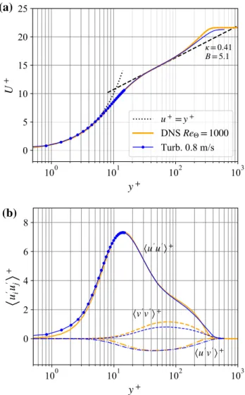
The turbulent velocity profile, normalized with inner (vis-cous) variables, is presented in Fig. 9a together with DNS data provided by Schlatter et al. (2009) for a Reynolds num-ber of Re
𝜃 =1000 . Corresponding profiles of the fluctuation
of the streamwise velocity ⟨u�u�⟩+ , the wall-normal velocity ⟨v�v�⟩+ and covariances
⟨u�v�⟩+ are shown in Fig. 9b. For
the most part, the measurement data for the turbulent case agrees well with the DNS data, except for the wall-normal fluctuations ⟨v�v�⟩+ that tend to be underestimated. This
could be attributed to spatial smoothing by the rather large length of the correlation window size in flow direction of 64 pixel corresponding to 1.07 mm or 39+ . Also the rather low
dynamic range of the wall-normal velocity component with a maximum standard deviation of ≈0.9 pixel can be affected
by pixel locking effects (Christensen 2004).
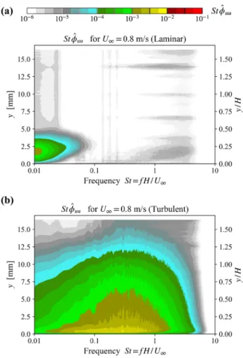
Spatially resolved power spectral densities (PSD) of the incoming velocity profiles are provided in Fig. 10. All quantities are normalized using the incoming velocity U∞
and the cube size H to allow a better comparison between the different flow conditions. The normalized frequency, defined as f̂
=fH U∞−1 , is equivalent to the Strouhal number
St . To better highlight small variations across the frequency
range, a pre-multiplication of the normalized spectral power
̂
𝜙 with the normalized frequency (i.e., Strouhal number St )
attenuates the typically higher PSD levels at lower frequen-cies while amplifying signals at the upper frequenfrequen-cies. The PSD for the turbulent in-flow indicates a maximum energy
(a)
(b)
Fig. 9 a Velocity profile for turbulent case at x= −52 mm upstream
of the cube normalized by inner variables (viscous scaling). b Cor-responding variances and co-variance of streamwise and wall-normal velocity components scaled with inner variables. Orange set of lines are from DNS data by Schlatter et al. (2009). For clarity symbols are only shown for y<20+
about 0.5 mm from the wall, near the inner turbulence peak ( y≈15+ or 0.4 mm), which is in agreement with the body of
literature. The spectral power gradually decreases through-out the vertical extent of the boundary layer. For the lami-nar in-flow condition, the flow, for the most part, is free of significant PSD levels, aside from a low frequency peak at
̂
f ≈0.01 (0.8 Hz) at a wall distance of y≈2 mm ≈0.4𝛿99 .
This low-frequency power does not seem to influence the flow around the cube as it cannot be detected in any of the spectra presented in the results section (see Sect. 3.2). The source of this spectral power is believed to be a low fre-quency modulation which might stem from water tunnel pumping and/or structure vibration eigenfrequencies with its respective receptivities of the laminar boundary layer. The signal is present at the same position for all but the lowest laminar Reynolds number with U∞=0.2 m/s.
3.2 TR‑PIV for 2D‑2C velocity fields
The following figures provide information of the flow around the cube exemplified for the case at U∞=0.8 m/s which
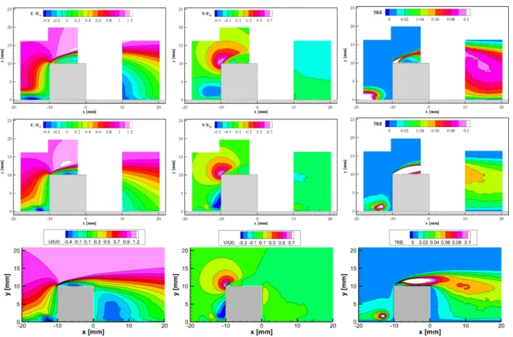
allows a comparison between experiment and LBM simula-tion. In Fig. 11 interesting flow features can be observed: For the turbulent flow case corresponding to 𝛿∕H=1.12 the
mean reattachment point downstream of the flow separation in the cube wake is located at x≈15 mm ( x∕H=1.5 ), while
it shifts further downstream to x≈18.5 mm ( x∕H=1.85 )
for the laminar condition with 𝛿∕H=0.44 .
Diaz-Dan-iel et al. (2017) provided the closest DNS with respect to present conditions and they gave a reattachment point value for the turbulent case at x∕H=1.5 and a stagnation
point value slightly above the wall for the laminar case at
x∕H=0.93 . For the turbulent case the value agrees very
well with our finding despite the difference in the Reynolds numbers ( Re
H=3000 for DNS compared to 8000 for the
experiment). Aside from the Reynolds number difference, the lower ratio of 𝛿∕H=0.44 for the present laminar case
also might contribute to a more extended mean recirculation bubble of up to x∕H=1.85 compared to the DNS which
is based on a ratio of 𝛿∕H=1 . On the other hand, for the
present laminar case at Re
H=2000 with a
correspond-ing 𝛿∕H=0.74 , the reattachment point shifts upstream to
x∕H=1.2 (see Fig. 22) which is closer to the DNS result
provided at ReH=3000 . Furthermore, the vertical extent
of the separation bubble on top of the cube is larger for the laminar case which is caused by the larger deflection angle of the incoming flow at the upstream upper edge of the cube due to the narrower laminar boundary layer thickness.
Between the laminar and turbulent cases, the distribution of the turbulent kinetic energy (TKE) differs significantly. Whereas the TKE is typically defined as one half of the sum of the three velocity variances ⟨u′
iu′i
⟩ , the present TR-PIV
measurements only provide variances for the two in-plane velocity components u and v. The missing variance for the
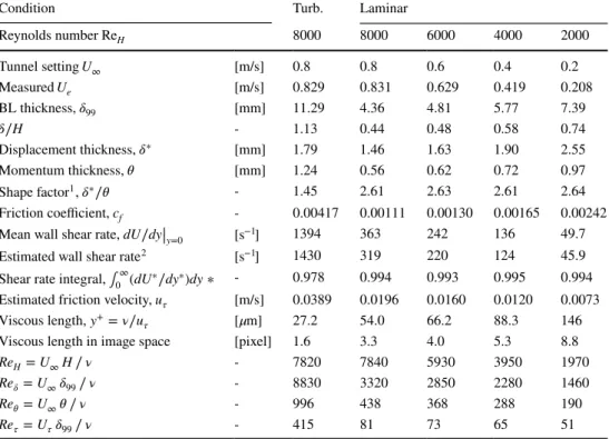
Table 2 Characteristic parameters of the boundary layer at upstream position, x= −52 mm (Pos.1)
1 Shape factor for Blasius profile: 𝛿∗∕𝜃 = 2.59.
2 Wall shear rate estimates for laminar cases are based on fit to Blasius solution
Condition Turb. Laminar
Reynolds number ReH 8000 8000 6000 4000 2000 Tunnel setting U∞ [m/s] 0.8 0.8 0.6 0.4 0.2 Measured Ue [m/s] 0.829 0.831 0.629 0.419 0.208 BL thickness, 𝛿99 [mm] 11.29 4.36 4.81 5.77 7.39 𝛿∕H - 1.13 0.44 0.48 0.58 0.74 Displacement thickness, 𝛿∗ [mm] 1.79 1.46 1.63 1.90 2.55 Momentum thickness, 𝜃 [mm] 1.24 0.56 0.62 0.72 0.97 Shape factor1 , 𝛿∗∕𝜃 - 1.45 2.61 2.63 2.61 2.64 Friction coefficient, cf - 0.00417 0.00111 0.00130 0.00165 0.00242 Mean wall shear rate, dU∕dy||y=0 [s−
1] 1394 363 242 136 49.7
Estimated wall shear rate2
[s−1
] 1430 319 220 124 45.9 Shear rate integral, ∫∞
0 (dU∗∕dy∗)dy∗ - 0.978 0.994 0.993 0.995 0.994 Estimated friction velocity, u𝜏 [m/s] 0.0389 0.0196 0.0160 0.0120 0.0073
Viscous length, y+
= 𝜈∕u𝜏 [𝜇m] 27.2 54.0 66.2 88.3 146
Viscous length in image space [pixel] 1.6 3.3 4.0 5.3 8.8
ReH=U∞H∕ 𝜈 - 7820 7840 5930 3950 1970 Re𝛿=U∞𝛿99∕ 𝜈 - 8830 3320 2850 2280 1460
Re𝜃=U∞𝜃 ∕ 𝜈 - 996 438 368 288 190
out-of-plane component ⟨w′w′⟩ is estimated as the mean of
the measured variances such that the TKE is approximated by 3
4(⟨u
�u�⟩
+⟨v�v�⟩) . The turbulent flow case exhibits larger
values of the (TKE) in the cube’s shear layer on top of the flow separation, whereas they are reduced almost by one half in the wake region compared to the laminar condition. A distinct point of high TKE is visible upstream of the cube close to the wall for the turbulent case which can be identi-fied as the point upstream of the first-order horse-shoe vortex origin. Here a dynamic bi-modal vertical velocity PDF has been previously documented by Yakhot et al. (2006a).
The differences between the TKE values in the cube wake for the two boundary layer flow types can be visualized as well by the two corresponding time traces of the stream-wise and wall-normal velocity components at the position of the mean reattachment point for the turbulent case near
x∕H=1.5 . Here, a higher dynamics of streamwise velocity
and specifically of small scale wall-normal velocity events with strong positive and negative values can be recognized for the laminar in-flow condition shown in Fig. 13. For the
turbulent in-flow condition corresponding time traces, pro-vided in Fig. 14, the wake dynamics are less pronounced and spatially and temporally smoother (Fig. 12). Note that the differences of the data resolution between the time traces of the incoming laminar (Fig. 13) and turbulent (Fig. 14) flow case is caused by the lower temporal resolution of the laminar TR-PIV measurements.
The mean flow field resulting from the LBM simula-tion of the turbulent case are provided in Fig. 11, bottom row. The simulation results exhibit a very similar distribu-tion structure for both velocity components and the TKE in comparison to the corresponding time resolved PIV result (Fig. 11, middle row). This agreement can also be seen in the streamlines in Fig. 25 where the different structures are well reproduced in size and position for the horseshoe vor-tex upstream of the cube, for the recirculation bubble on the top face and in the wake. While the TKE distribution obtained from the measurements relies on an approxima-tion using only two velocity components, Fig. 12 provides an additional side-by-side view of the velocity variances of the in-plane velocity components (i.e., u and v) obtained from experiment and simulation. This also confirms that the chosen TKE approximation is viable for this configuration along the symmetry plane at z=0.
The influence of the in-flow conditions on the wake dynamics can also be observed in the power spectra obtained along a wall-normal line at x=15 mm. Figure 15 provides
normalized power spectra of the streamwise velocity for the two conditions, pre-multiplied by the non-dimensional fre-quency St to more clearly highlight differences. Noteworthy,
is a pronounced signal for the laminar condition at a non-dimensional frequency of St≈0.1 which extends all the way
to the wall. This frequency previously has been documented in literature for a cube in turbulent channel flow (Meinders et al. 1999; Yakhot et al. 2006b) and is associated with peri-odic large-scale vortex shedding in the cube’s wake. Unlike the findings reported in the literature, the experimental data for the turbulent in-flow condition does not exhibit this pro-nounced frequency and rather has a much more broad-band power spectral density distribution peaking at St≈0.5 and y≈11 mm ( y∕H≈1.1 ). Spatially this spectral density peak
coincides with the peak TKE for both laminar and turbulent in-flow. On the other hand it is noteworthy that turbulent boundary layer and turbulent channel flows lead to vari-ous differences in the reported dynamics (Castro and Rob-ins 1977; Yakhot et al. 2006b) such that the discrepancies observed here are not surprising.
3.3 Time‑resolved 3D‑3C velocity and acceleration fields
Evaluation of the complete volumetric data set given in Table 1 was performed successfully using Lagrangian
Fig. 10 Pre-multiplied frequency spectra of the streamwise velocity profile at x= −52 mm upstream of cube for the laminar (a) and tur-bulent in-flow condition (b)
particle tracking (LPT) by the Shake-The-Box (STB) algo-rithm (Schanz et al. 2016). Figures. 16 and 17 show results for a case with laminar in-flow conditions at U∞=0.4 m/s.
Within the reconstructed volume around 70,000 particles were instantaneously tracked over many time steps and the velocity and acceleration resp. material derivative informa-tion was computed directly from the continuous temporal B-spline fit function (TrackFit). For this case 22,050 suc-cessive images at a recording frequency of 750 Hz are avail-able (see Tavail-able 1). Figure 16, top, shows particle tracks in proximity of the wall at 0<y<1.2 mm are color coded by
streamwise velocity. On the right of Fig. 16 at U
∞=0.2 m/s
tracks are shown for a slightly larger wall parallel slice color coded by wall normal acceleration, which nicely highlights the horse shoe vortices present in front and on both sides of the cube close to the wall.
Measuring Lagrangian acceleration by STB a dense distribution enhances the quality of the FlowFit data assimilation scheme: On the left hand side of the imposed Navier–Stokes momentum equation. These input values directly allow the calculation of accurate instantaneous 3D
pressure distributions (Huhn et al. 2018). The upper left of Fig. 17 shows a side view of a central slice at z=0 with
3 mm thickness comprising 60 successive time-steps. Here, the motion of particles approaching the cube within the incoming boundary layer of the flow can be observed. The particles are being decelerated and deflected by the adverse pressure gradient field in front of the cube (see Fig. 26) and then are either transported over the cube when arriv-ing above the stagnation point on the cube’s front surface or towards the wall if below. Particles deflected downward either move into the horseshoe vortex and then around the cube as indicated in Fig. 16, bottom, or when pushed even closer to the wall, they tend to travel in an upstream direction within a thin layer.
Many particles remain close to the wall and travel around the cube at a surprisingly large radius and low velocity (see Fig. 16). Large, elongated vortices are visualized by the tra-jectories, bent around the cube (see Figs. 16 and 17 right). Separation bubbles are present at the three streamwise faces of the cube (best visible in Fig. 17 left up for the top face), where fluid flows backwards, until the vortex structures are
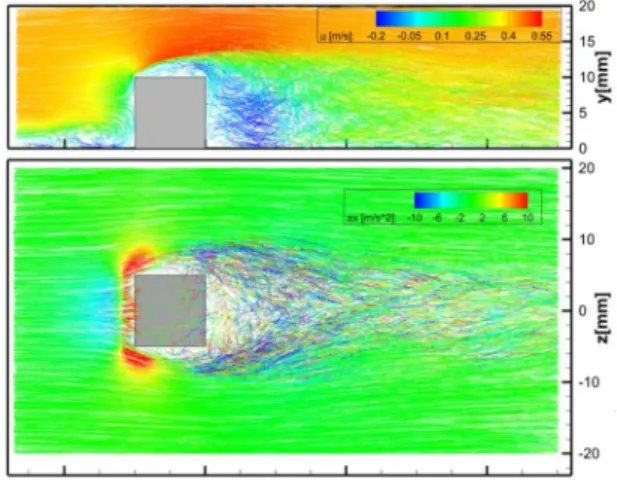
Fig. 11 Flow fields around the cube at center plane ( z=0 ) obtained
with TR-PIV for the laminar flow case (top row) and turbulent in-flow case (middle row). Bottom row shows corresponding in-flow fields obtained with LBM for the turbulent case. Mean streamwise velocity
(left column), mean wall-normal velocity (middle column) and turbu-lent kinetic energy (right column), all normalized by the in-coming flow velocity U∞=0.8 m/s
carried away by the suction along the sharp shear layer that is created at the edges of the cube. Here, the highest acceler-ations are seen (see Fig. 17, bottom left). Strongly turbulent flow is generated in the wake of the cube specifically for the higher laminar BL flow velocities.
Using the FlowFit algorithm, the densely tracked parti-cles can be used in conjunction with physical regulariza-tions to interpolate the velocity, acceleration and pressure field onto a regular grid. As a result the temporally resolved
3D velocity and acceleration gradient tensor is available. Figure 17, right shows an instantaneous FlowFit result with iso-surfaces of vorticity. The cube is covered by connected regions of shear vorticity that quickly break up into vorti-ces of different scales, as the flow becomes turbulent. The bent vortices surrounding the cube in upstream direction that were already visible in Fig. 17, right can now be clearly identified. A large horseshoe vortex, surrounding the lower part of the cube that breaks up when secondary hairpin-type
Fig. 12 Comparison between TR-PIV (top row) and LBM results (bottom row) for the velocity variances: streamwise velocity (left column) and wall-normal velocity (right column) at center plane ( z=0 ), all normalized by the in-coming flow velocity U∞=0.8 m/s
Fig. 13 Portion of the velocity profile time record for the
lami-nar condition downstream of the cube at x∕H=1.5 (Pos.3) at U∞=0.8 m/s showing streamwise velocity (top), wall-normal
veloc-ity (bottom), both normalized by the incoming bulk velocveloc-ity U∞
Fig. 14 Portion of the velocity profile time record for the turbulent
condition downstream of the cube at x∕H=1.5 (Pos.3) showing
streamwise velocity (top), wall-normal velocity (bottom), both nor-malized by the incoming bulk velocity U∞
vortices are developed, is visible. Two other flow field exam-ples visualized by 3D vorticity iso-contour surfaces of the laminar case with U∞=0.8 m/s are given in Fig. 18.
In Fig. 18, the influence of the cube on the stability of the laminar flow is clearly visible along the generated shear layers and the horse-shoe vortices. In all related shear flow regions first typical Kelvin-Helmholtz instabilities gener-ate waviness leading to the rapid evolution of hairpin-like vortices. The downstream development of similar vortex structures on top of the horseshoe vortices is as well visible on both sides of the cube. The hairpin-like vortices evolve in wall-normal and spanwise direction and are convected downstream inducing entrainment events through the wake shear layer and a spanwise growing of a turbulent wedge.
The higher wake dynamics of the laminar in-flow condi-tion in comparison to the turbulent case can also be observed in the spectra presented in Fig. 15. For the laminar case at
U
∞=0.8 m/s a strong signal is present at St= ̂
f ≈0.1 which
can be attributed to large scale vortex shedding from the cube and can be observed all the way to wall. This value is consistent with the value of St=0.104 reported in the
literature (Yakhot et al. 2006b; Meinders et al. 1999). For the turbulent case, the vortex shedding is much less pro-nounced and shifted toward higher frequencies, while the overall PSD is roughly reduced by a factor of 2. Closer to the wall the wake dynamics of the laminar case are also more pronounced in comparison to the turbulent condition which agrees with the visual impression obtained from Figs. 13
and 14.
Fig. 15 Pre-multiplied spectra of the normalized streamwise velocity
u at x∕H=1.5 in the wake of the cube for laminar BL in-flow (a) and turbulent BL in-flow (b), both at U∞=0.8 m/s. The dashed line
rep-resents St=0.104 as reported in literature
Fig. 16 a Particle tracking results for U∞=0.4 m/s laminar in-flow,
displaying a slice close to the wall ( y=0−1.2 mm) color-coded by
streamwise velocity. b 3D-STB result obtained at laminar in-flow of U∞=0.2 m/s with slice through volume at y=0−3.5 mm with
color coding of the wall-normal acceleration. Animated versions of these figures are available in the supplementary material
Fig. 17 3D STB result for U∞=0.4 m/s laminar in-flow. a Side
view on a 3 mm slice at the mid plane of the cube. Particle tracks of 60 successive time-steps, color-coded by streamwise velocity. b
View from above on a 1.3 mm slice near the top of the cube ( y=
9.5–10.8 mm), color-coded by streamwise acceleration. c Instantane-ous snapshot of vorticity iso-surfaces ( |𝜔|=170s−1 ) color coded by
u-velocity, as calculated by FlowFit from the STB tracking results. An animated version of the iso-vorticity rendering is available in the supplementary material
Fig. 18 Two successive time-steps of U∞=0.8 m/s laminar case with vorticity iso-surfaces by FlowFit
Fig. 19 Portion of the velocity time record of the wall-normal veloc-ity above the cube at x∕H= −0.4 (Pos.2) for the laminar condition
(top) at U∞=0.4 m/s and turbulent condition at U∞=0.8 m/s
(bot-tom). Both plots are normalized by the incoming bulk velocity U∞
Fig. 20 Pre-multiplied spectra of the wall-normal velocity above to
cube at x∕H= −0.4 for laminar BL in-flow (a) and turbulent BL in-flow (b)
Turning attention to the shear layer above the cube, the flow exhibits considerable differences between laminar and turbulent in-flow conditions. For the turbulent condition the shear layer dynamics are very random as testified by both the velocity time record (Fig. 19, bottom) and the associ-ated broad-band frequency spectrum (Fig. 20, bottom). The laminar in-flow, on the other hand, exhibits a shear layer with a non-periodic transition to short-lived, fine-scale vor-tex shedding whose signature can be seen in vertical velocity component of the time record in Fig. 19, top. The frequency of this intermittent shedding peaks at St≈2 and is more than
an order of magnitude higher than the large scale shedding of St≈0.1 observed in the wake of the cube.
3.4 3D bin‑averaging results
A straight-forward statistical approach which preserves the high spatial resolution of the available particle tracking data while being adaptable to the threshold requirements of statistical convergence of the different one- or multi-point statistics is the so called “bin-averaging” method. Here the complete data set of about 22, 000 time steps of the tracking results are used to build a dense grid of 9.85×10⁶ bins with
an individual cubic bin size of 0.253mm3 . A result of the
converged mean flow field color coded by the streamwise velocity is given in Fig. 21 and shows a volumetric overview of the mean flow field by three orthogonal slices through the domain. It represents a small part of the maximal possible
Fig. 21 Result of 3D mean velocity field for the laminar BL flow case at U∞=0.2 m/s based on bin-averaging approach and visualized
by three perpendicular vector planes color coded by the streamwise velocity. Data set consists of nearly 107
volume bins of size 0.253mm3
Fig. 22 Bin averaged 3D velocity fields of the laminar test cases at in reading order increasing U∞=[0.2; 0.4; 0.6; 0.8] m/s and
correspond-ing Re
H=[2000; 4000; 6000; 8000]. Color coded streamwise
veloci-ties uat four extracted planes, with the horizontal plane at y=1 mm above the wall. Iso-contour surfaces enclose negative u-velocity val-ues. Note the differences in the color bar
Fig. 23 Result of 3D mean velocity field for laminar boundary layer flow case at U∞=0.2 m/s based on bin-averaging approach (see
Fig. 21) and visualized by a vector plane at y=0.5 mm (indicative of
the wall shear stress distribution) (a) and at y=5 mm (b), both color coded by the streamwise velocity component
spatial dynamic range, which is given with the positional accuracy of the individual tracks ( ≈0.1 pixel, here ≈4𝜇 m)
and limited only by the possible number of statistical inde-pendent samples per bin. By applying symmetry conditions even higher spatial resolutions can be achieved (Fig. 22).
In Fig. 23, left a wall-parallel slice of the bin averaging result of Fig. 21 is given at y=0.5 mm. For this specific case
at U∞=0.2 m/s or ReH=2000 with 𝛿∕H=0.74 the
dis-played flow structure at the wall is a good and direct approxi-mation of the mean skin friction velocity vector distribution. The flow pattern and vector field of the near wall mean flow is very similar to the DNS results shown for ReH=3000 in
the paper by (Diaz-Daniel et al. 2017, Fig. 1). For calcula-tion of the overall flow induced drag the skin friccalcula-tion field could be integrated together with those at the surfaces of the cube itself. Access to a direct estimation of the surface
drag based on the flow field around an obstacle is considered a very interesting novelty for aerodynamic investigations. Together with the pressure field estimation, based on the same bin averaging result using the FlowFit approach in the entire volume (see Fig. 26), the classical drag estimation approach based on a wake integration of the pressure deficit can be tested and validated at different downstream wake distances allowing a quantitative comparison to the direct drag integration proposed here. This proposed approach might be addressed in a future campaign. It has not been attempted here because the volume size was not sufficient in span- and streamwise directions and the very small bin size (at least in wall-normal direction) required for estimating
Fig. 24 Mean velocity streamlines from TR-PIV measurements for
laminar boundary layer flow case at U∞=0.2 m/s at z=0 mm (a)
and corresponding streamlines cut of 3D STB bin-averaging result (b)
Fig. 25 Comparison between TR-PIV (a) and LBM results (b). The streamlines are plotted at the symmetry plane z=0 mm for the
turbu-lent test case at U∞=0.8 m/s
Fig. 26 Mean 3D pressure field iso-surfaces around the cube based
on bin-averaging (a) and the same pressure field color coded on iso-surfaces of mean streamwise velocity (b)
the average skin friction velocity field at all model surfaces would require a significantly higher number of samples to achieve statistical convergence.
A direct comparison of the streamlines upstream of the cube obtained from the TR-PIV measurement 3D bin-averaging and 3D STB data is provided in Fig. 24 for
U∞=0.2 m/s in the center-plane. Furthermore a comparison
between the time-averaged TR-PIV measurements and the LBM simulation is provided in Fig. 25, for the turbulent case at U
∞=0.8 m/s. The upstream horseshoe vortex, the
separated flows at the corners and the recirculation region sizes are well defined and reproduced by the simulation. The deceleration of the flow below the cube’s stagnation point generates a hierarchy of horse-shoe vortices with negative spanwise vorticity close to the wall. In between the rollers smaller counter-rotating vortices are induced with reduced vorticity magnitudes. In the 3D bin-averaged result the streamlines of the first-order and strongest horse-shoe vor-tex closest to the cubes front surface “escape” in spanwise direction (empty core) due to a small asymmetry of the aver-aged flow. This might be caused by the low frequency quasi-periodic oscillations in the wake downstream of the cube or by the inherent asymmetries of bluff-body wakes (Fig. 26).
3.5 Reynolds number effects for the laminar test cases
With increasing Reynolds numbers the flow around the cube changes mainly for three reasons: (a) the momentum of the incoming flow increases, while (b) at the same time the laminar boundary layer thickness decreases and (c) the dynamics of the transitional and turbulent flow struc-tures along the shear layers and in the wake increases. At higher flow velocities this leads to higher accelerations at the cube front edges and consequently to an increase of the flow separation domain size around the cube’s side and top faces as well as in the wake. The volume of negative mean streamwise velocities u, indicated by the blue iso-contour surfaces in Fig. 22, increase both in spanwise—as well as in streamwise direction with increasing Reynolds number. Furthermore, the extracted horizontal plane close to the wall shows an increasing upstream extension of an area of nega-tive streamwise velocities for the higher Reynolds number cases indicating the influence of the first, second and third generation of horse-shoe vortices induced in front of the cube (see Fig. 24). In the same extracted horizontal plane and in the middle crossflow plane (YZ-plane) the increase of the wall-normal momentum exchange due to the pres-ence of the streamwise aligned lateral horseshoe vortices can be clearly seen. More general flow features can also be observed in the 3D flow bin-averaged images of Fig. 22.
The transitional and turbulent flow structures in particu-lar (e.g., wavy and hairpin-like vortices in Figs. 17 and 18)
which are developing along the shear layers enveloping the negative u-velocity values and along the lateral cube faces the horse-shoe vortices change their character in the wake of the cube with increasing Reynolds number. As the range of scales and the amplitude of Reynolds stress events, which guide the momentum exchange through the mean shear lay-ers, increase with Reynolds number, also the dynamics of the flow separation region in the wake is affected: for the two steps from Re
H=2000 to 4000 and 6000, a significant
streamwise increase of the separation bubble in the cube wake can be observed with mean reattachment point mov-ing from x∕H=1.2 to 1.8). Increasing the conditions from Re
H= 6000–8000 only a small shift of the reattachment
point is observed by moving from x∕H=1.8 to 1.85). This
can be explained for the first two steps by the overall increase of the momentum deficit induced by the presence of the cube and the reduced turbulent exchange in the shear layers, while the last reduced step size is caused by a significant increase of momentum exchange driven by vortical structures (see Fig. 13) through the shear layers due to an already fully developed turbulent wake at the higher Reynolds numbers. A detailed view into the dynamics of the interaction of shear layer development and the complete wake would need fur-ther analysis of the different spectra for velocity and pressure fluctuations, preferably in 3D space. This would require a full set of time series of FlowFit data assimilation results together with the TR-PIV results combined with advanced modal decomposition analysis which are beyond the scope of the present paper and will be reserved for future work.
3.6 TR‑PIV versus 3D STB: Pros and Cons
In the present experimental investigation two particle based measuring techniques were applied in a complementary manner regarding spatial (and temporal) resolution and statistical convergence of the measured quantities. TR-PIV measurements were performed locally to obtain velocity ‘profiles’ of the mean velocity fields and related higher-order statistics. Additionally, the spatio-temporally grid-ded data of the time-resolved 2C vector fields enable the determination of related frequency spectra. TR-PIV profile measurements can be done with a single camera setup at high magnifications with a simple 2D calibration and high sample rates. The combined advantages on the hardware side are an increase of the camera frame rate with the reduc-tion of the CMOS camera sensor resolureduc-tion in one dimen-sion to a “2D column” imaging particles within a narrow collimated the laser light sheet. The collimation allows the local light energy density to be increased sufficiently for the illumination of small tracer particles even at high repetition rates. The employed cross-correlation based PIV analysis is fast, robust and well established, but induces low-pass spatial filtering effects (Raffel et al. 2018, Ch.6). In future