Nosetip Bluntness Effects on Transition at Hypersonic Speeds:
Experimental and Numerical Analysis
Pedro Paredes,∗
National Institute of Aerospace, Hampton, VA 23666, USA
Meelan M. Choudhari,† Fei Li,‡
NASA Langley Research Center, Hampton, VA 23681, USA Joseph S. Jewell,§ Roger L. Kimmel,¶
U.S. Air Force Research Laboratory, Wright-Patterson Air Force Base, OH 45433, USA Eric C. Marineau,‖
AEDC White Oak, Silver Spring, MD 20903, USA Guillaume Grossir∗∗
von Karman Institute for Fluid Dynamics, B-1640 Rhode-St-Genèse, Belgium
The existing database of transition measurements in hypersonic ground facilities has estab-lished that the onset of boundary layer transition over a circular cone at zero angle of attack shifts downstream as the nosetip bluntness is increased with respect to a sharp cone. However, this trend is reversed at sufficiently large values of the nosetip Reynolds number, so that the transition onset location eventually moves upstream with a further increase in nosetip blunt-ness. This transition reversal phenomenon, which cannot be explained on the basis of linear stability theory, was the focus of a collaborative investigation under the NATO STO group AVT-240 on Hypersonic Boundary-Layer Transition Prediction. The current paper provides an overview of that effort, which included wind tunnel measurements in three different facil-ities and theoretical analysis related to modal and nonmodal amplification of boundary layer disturbances. Because neither first and second-mode waves nor entropy-layer instabilities are found to be substantially amplified to initiate transition at large bluntness values, transient (i.e., nonmodal) disturbance growth has been investigated as the potential basis for a physics-based model for the transition reversal phenomenon. Results of the transient growth analysis indicate that stationary disturbances that are initiated within the nosetip or in the vicinity of the juncture between the nosetip and the frustum can undergo relatively significant nonmodal ∗Research Engineer, Computational AeroSciences Branch, NASA LaRC. AIAA Senior Member
†Research Scientist, Computational AeroSciences Branch. AIAA Associate Fellow ‡Research Scientist, Computational AeroSciences Branch.
§Research Scientist, (Spectral Energies, LLC), AFRL/RQHF. AIAA Senior Member ¶Principal Aerospace Engineer, AFRL/RQHF. AIAA Associate Fellow
‖Currently Program Officer for Hypersonics at the Office of Naval Research. AIAA Senior Member ∗∗Post-doctoral Fellow, Aeronautics and Aerospace Department
amplification and that the maximum energy gain increases nonlinearly with the nose radius of the cone. This finding does not provide a definitive link between transient growth and the onset of transition, but it is qualitatively consistent with the experimental observations that frustum transition during the reversal regime was highly sensitive to wall roughness, and furthermore, was dominated by disturbances that originated near the nosetip. Furthermore, the present analysis shows significant nonmodal growth of traveling disturbances that peak within the entropy layer and could also play a role in the transition reversal phenomenon.
Nomenclature
E = total energy norm
F = disturbance frequency
G = energy gain
ht = total enthalpy
hξ = streamwise metric factor
hζ = spanwise metric factor
J = objective function
K = kinetic energy norm
k = peak-to-valley roughness height
L = reference length
m = azimuthal wavenumber
M = Mach number
N = Logarithmic amplification factor ¯
q = vector of base flow variables ˜
q = vector of perturbation variables ˆ
q = vector of amplitude variables Rek k = roughness-height Reynolds number
Re∞ = freestream unit Reynolds number
ReRN = Reynolds number based on nose radius
ReξT = transition Reynolds number based on freestream velocity and transition location
rb = local radius of axisymmetric body at the axial station of interest
RN = nose radius
Tw = wall temperature
Tw,ad = adiabatic wall temperature
(u,v,w) = streamwise, wall-normal, and spanwise velocity components (x,y,z) = Cartesian coordinates
α = streamwise wavenumber
δh = boundary layer thickness
δS = entropy layer edge
κ = streamwise curvature
ω = disturbance angular frequency
ρ = density
(ξ, η, ζ) = streamwise, wall-normal, and spanwise coordinates
∆ξ = streamwise interval considered for optimal growth analysis
∆S = entropy increment
φ = angular coordinate
θ = cone half-angle
M = energy weight matrix
Superscripts ∗ = dimensional value H = conjugate transpose Subscript ∞ = freestream value 0 = initial position 1 = final position j = juncture location T = transition location Abbreviations
AFRL = Air Force Research Laboratory
AEDC = Arnold Engineering Development Complex DNS = direct numerical simulation
DPLR = data parallel-line relaxation FST = freestream turbulence
LIF = laser-induced fluorescence PNS = parabolic Navier-Stokes equations PSE = parabolized stability equations
I. Introduction
Laminar-turbulent transition of boundary-layer flows can have a strong impact on the performance of hypersonic vehicles because of its influence on the surface skin friction and aerodynamic heating. Therefore, the prediction and control of transition onset and the associated variation in aerothermodynamic parameters in high-speed flows is a key issue for optimizing the performance of the next-generation aerospace vehicles. Although many practical aerospace vehicles are blunt, the mechanisms that lead to boundary-layer instability and transition on blunt geometries are not well understood as yet. A detailed review of boundary layer transition over sharp and blunt cones in a hypersonic freestream is given by Schneider [1]. As described therein, both experimental and numerical studies have shown that the modal growth of Mack-mode instabilities (or, equivalently, the so called second-mode waves) is responsible for laminar-turbulent transition on sharp, axisymmetric cones at zero angle of attack. Studies have also shown that increased nosetip bluntness has a stabilizing effect on the amplification of Mack-mode instabilities, which is consistent with the observation that the onset of transition is displaced downstream as the nose bluntness is increased. However, while the boundary layer flow continues to become more stable with increasing nose bluntness, experiments indicate that the downstream movement in transition actually slows down and eventually reverses as the nose bluntness exceeds a certain critical range of values. The observed reversal in transition onset at large values of nose bluntness is contrary to the predictions of linear stability theory, and therefore, must be explained using a different paradigm. While no satisfactory explanation has been proposed as yet, one of the physical effects that have been suspected to cause this transition reversal is the role of surface roughness.
Earlier measurements related to the effect of nose bluntness on frustum transition over hypersonic blunt cones have been thoroughly documented by Stetson [2]. He concluded that the details of the nose tip flow played an important role in the transition reversal process, even though the onset of transition occurred significantly farther downstream over the frustum of the cone. Stetson [2] also observed that the measured transition locations within this regime were not easily reproducible across different runs. At a fixed set of freestream conditions, transition onset was found to vary across a wide range of frustum stations, and at times, the boundary layer flow remained laminar over the entire cone. Nonaxisymmetric transition patterns were observed even at zero angle of attack, and the measured length of the transition zone was much larger than that for cones with smaller values of nose bluntness. Finally, Stetson observed that frustum transition in the transition-reversal regime was highly sensitive to surface roughness in the nosetip region. For smaller nosetip bluntness prior to transition reversal, the surface finish on the nosetip (or the frustum) appeared to have
no effect on frustum transition. Polishing the blunt nosetip before the wind tunnel run for the large bluntness cones resulted in either higher frustum transition Reynolds numbers or a completely laminar flow over the model. Primarily on the basis of this last observation, Stetson speculated that frustum transition for large bluntness cones was dominated by disturbances originating near the nosetip. Therefore, roughness-induced transient growth appears to be a reasonable explanation for the transition-reversal phenomena in large bluntness cones at high speeds.
Historically, the term “bypass transition” has been used to identify transition paths that cannot be explained via modal amplification of small-amplitude disturbances [3]. Well-known examples of bypass transition include the transition due to high levels of freestream disturbances, as for example, in turbomachinery, or the subcritical transition observed in Poiseuille pipe flow experiments [4–6], transition due to distributed surface roughness on flat plates [7, 8] or cones [9], and subcritical transition observed on spherical forebodies [10–13]. Because of the strongly favorable pressure gradient over blunt bodies such as hemispherical nose tips and spherical segment capsules, the laminar boundary layer is highly stable; and hence, the observed onset of transition on such bodies has been known as the “blunt-body paradox”. In recent years, the phenomenon of transient, nonmodal amplification of disturbance energy has emerged as a possible explanation for many cases of bypass transition. Mathematically, the transient, nonmodal growth is associated with the nonorthogonality of the eigenvectors corresponding to the linear disturbance equations. Physically, the main growth mechanism corresponds to the lift-up effect [14–16], which results from the conservation of horizontal momentum in the course of spanwise varying wall-normal displacement of the fluid particles. The actual growth in any given scenario is determined by the details of the external disturbance environment. However, an upper bound on the magnitude of energy gain via transient growth can be predicted by using the so-called optimal growth theory, which is typically formulated to maximize the disturbance growth across a specified interval of streamwise locations. Regardless of the flow Mach number [17, 18], the disturbances experiencing the highest magnitude of transient growth have been found to be stationary streaks that arise from initial perturbations in the form of streamwise vortices. Schmid & Henningson [19] and Schmid [20] provide a thorough review of the transient growth theory and the earlier results from the literature.
Reshotko & Tumin [21] were able to successfully correlate the transition data from several wind tunnel experiments involving subcritical, nose tip transition by using a semiempirical correlation derived from the optimal transient growth theory, which provides an upper bound on the magnitude of transient growth under suitable constraints. Reshotko & Tumin [21] extended the ideas from Anderson et al. [22], who had investigated subcritical transition in a flat plate boundary layer due to moderate to high levels of freestream turbulence (FST) and had derived a correlation based on the optimal growth of boundary layer disturbances generated by the FST. Based on the hypothesis that a similar disturbance growth could also be initiated by distributed surface roughness over hypersonic blunt forebodies, Reshotko & Tumin [21] were able to develop a semiempirical transition correlation by linking a critical disturbance amplitude required for the onset of transition with the roughness height parameter via a gain function based on the optimal growth framework. Even though the relevance of the linear, optimal disturbance growth concept to realistic, rough nose tips remains
to be established, their work provides the first physics-based model toward a potential resolution of the blunt-body paradox. Unlike other established models based on empirical curve fits that are valid for a specific subclass of datasets, Reshotko & Tumin’s optimal-growth-based transition criterion has been able to provide a reasonable correlation with the measurements in various wind tunnel and ballistic range facilities and for a broad range of surface temperature ratios. In follow-on work, Paredes et al. [23, 24] have revised the Reshotko & Tumin correlation by including the effects of nonparallel basic state evolution, curvature terms, and the variation of both inflow and outflow locations for the transient growth interval. Their results indicate that application of a more thorough theoretical framework reveals certain new features of optimal growth characteristics that were not indicated by the parallel framework used in the previous correlation. However, despite these changes, the constants in the transition correlation remain close to their original values.
Not withstanding the questions related to the physical relevance of optimal growth theory, the successful correlation of much of the available data by the Reshotko & Tumin correlation raises the possibility that a similar framework could also correlate (or, perhaps, explain) the observations of transition reversal over blunt cones. That possibility was investigated during a collaborative efforts under the NATO STO group AVT-240 on Hypersonic Boundary-Layer Transition Prediction focused on the problem of blunt cone transition and the potential role of transient growth in the transition reversal phenomenon. While the problems of blunt-body paradox and transition reversal over blunt cones share a key similarity by way of transition onset in the absence of (significant) modal instability, they also exhibit two major differences. First, the onset of transition in the latter case is typically observed over the frustum of the cone, as opposed to the nose tip in the case of blunt body paradox. As such, the transient growth characteristics of blunt cone boundary layers are also expected to be different, and in fact, more complex than those over a blunt nose without any frustum. Besides investigating the transient growth features over blunt cones, the NATO group’s effort also included wind tunnel measurements in both U.S. and Europe, and a preliminary study related to the effects of an azimuthally-periodic array of roughness elements located near the sonic location over the nose tip. The current paper provides an overview of the collaborative work including both theoretical analysis and experimental measurements. The layout of the paper is as follows. First, experimental transition measurements over blunt cones at hypersonic freestream speeds from the literature are summarized and compared in Section II. In Section III, we apply the transient growth analysis to hypersonic blunt cones for selected flow conditions that match the experimental studies relevant to the NATO effort [2, 25]. Those results were used to determine the azimuthal spacing between roughness elements for the experimental measurements of roughness effects within the transition reversal regime. Section IV outlines the preliminary findings from that experiment, while the summary and conclusions are presented in Section V.
II. Overview of Transition Measurements over Blunt Cones
The effect of nosetip bluntness on boundary-layer transition is often assessed by plotting the transition Reynolds number as a function of the nosetip radius Reynolds number where both Reynolds numbers are based on the freestream conditions. Figure 1(a) presents the Reynolds number at the start of transition (ReξT) as a function of the nosetip Reynolds number (ReRN) for the experiments by Stetson [2] in the Air Force Research Laboratory (AFRL) Mach 6 high-Reynolds-number facility withRN =sharp (A1), 0.5 (A2), 1.0 (A3), 1.5 (A4), 2.0 (A5), 2.5 (A6), 5.1 (A7), 7.6
(A8), 10.2 (A9), 12.7 (A10), and 15.2 mm (A11) cones; and by Aleksandrova et al. [26] in the Central Aerohydrodynamic Institute (TsAGI) UT-1M Ludwieg tube with withRN =0.5 (B1), 1 (B2), 2 (B3), 3 (B4), 4 (B5), 5 (B6), 6 (B7), 7 (B8),
8 (B9), 10 (B10), 12 (B11), and 14 mm (B12) cones. Both data sets are at a nominal freestream Mach number of 6 on straight 8◦half-angle cones. The data from Stetson displays two distinct regions referred to as “small bluntness” where
the transition location moves downstream with increased bluntness, and “large bluntness” where the transition location rapidly moves upstream. The data from Aleksandrova et al. [26] (indicated by star symbols) has a positive slope (small bluntness behavior) up to a criticalReRN of 1.3×10⁵. Beyond this critical value, the transition appears to depend on uncontrolled disturbances due to nosetip roughness. In the critical region, groups of points clustered by nosetip radii of 3, 4, 5, 12, and 14 mm exhibit a decrease in the transition Reynolds number with an increasing nosetip Reynolds number, which is indicative of transition reversal. With the exception of the sharp and the 0.5 mm nosetips that consist of steel inserts, the cone model and nosetip inserts were made of AG-4 composite material. The roughness height of the AG-4 material was not specified by the authors, but is expected to be rougher than polished steel. The shape of the transition front, which was quantified using temperature-sensitive paint, revealed turbulent wedges at Reynolds numbers above the critical value. The authors attribute the formation of such wedges to the presence of uncontrolled nosetip roughness. The experiments from Aleksandrova et al. [26] illustrate that surface roughness has a significant effect on the emergence of the transition reversal. In Stetson’s Mach 6 experiments [2], the nominal model surface finish had a root-mean-square (rms) value of 15µin. (0.38 µm) and blunt nosetips were polished before each run. The polished nosetips most likely explain why the small bluntness behavior was extended to nosetip Reynolds numbers slightly above 9.0×10⁵in Stetson’s experiments. The sensitivity of frustum transition to roughness at high nosetip Reynolds numbers was investigated by Stetson by adding 45−50µin. (1.14−1.27µm) rms roughness on the 0.6 in. (15.2 mm) nosetip. The added roughness caused early frustum transition.
Figure 1(b) presents the Reynolds number at the start of transition as a function of the nosetip Reynolds number for three sets of experiments at nominal freestream Mach numbers between 9 and 10 on straight slender cones. The plot includes the experiments of Stetson [2] in Tunnel F at Mach 9 on 7◦half-angle cones withR
N =sharp (C1), 1.5
(C2), 4.5 (C3), 7.5 (C4), 10.5 (C5), 14.0 (C6), 22.5 (C7), 55.4 (C8); of Marineau et al. [25] in Tunnel 9 at Mach 10 on 7◦half-angle cones with R
N =0.15 (D1), 5.1 (D2), 9.5 (D3), 12.7 (D4), 25.4 (D5), and 50.1 mm (D6); and that of
Softley et al. [27, 28] in the G.E. shock tunnel on 5◦half-angle cones withR
104 105 106 107 ReRN 106 107 108 R eξ T A1 A2 A3 A4 A5 A6 A7 A8 A9 A10 A11 B1 B2 B3 B4 B5 B6 B7 B8 B9 B10 B11 B12 (a) 102 103 104 105 106 107 ReRN 106 107 108 R eξ T C1 C2 C3 C4 C5 C6 C7 C8 D1 D2 D3 D4 D5 D6 E1 E2 E3 E4 E5 E6 (b)
Fig. 1 Transition Reynolds number based on freestream as a function of the nose Reynolds number at (a) Mach 6and (b) Mach9to10which illustrates the effect of bluntness and the transition reversal.
(E4), 19.1 (E5), and 25.4 mm (E6). As seen at Mach 6, the Mach 10 data also displays the small bluntness and large bluntness regions. The boundary between the large bluntness and small bluntness occurs at varying Reynolds numbers of approximately 1.2×10⁵, 3.9×10⁵, and 9.0×10⁵, respectively, for Softley, Marineau, and Stetson. The reason for the variation in the critical Reynolds numbers among the three data sets is not clear, since the respective experiments report similar surface finishes of 30, 32, and 40µin. (0.76, 0.81, and 1.02µm). Just like Stetson, Softley and Marineau also polished the nosetip prior to each run, but from the results it appears that the polished surface finish might have been smoother in Stetson’s experiment.
As noted by Stetson [29], the use of “small bluntness” and “large bluntness” when discussing nosetip bluntness effects can be misleading, as the bluntness effect is related not only to the physical dimensions of the nosetip, but also to where transition occurs with respect to the nosetip. As discussed by Muir and Trujillo [30], the nosetip Reynolds number does not properly account for the various effects of the nosetip radius and unit Reynolds numbers. Stetson and Rushton [31] introduced the entropy-swallowing length as a parameter to relate the transition location to nosetip bluntness effects. Using Rotta’s correlation [32], the entropy-swallowing length is found to be a function of(Re∞)1/3
and(RN)4/3. One disadvantage of the entropy-swallowing length as a correlation parameter is that it cannot be easily
defined for arbitrary geometries. Moreover, the blunt cone data is usually correlated by normalizing the transition locations (location or Reynolds numbers) on blunt cones by the transition length on sharp cones in order to remove unit Reynolds number effects. Such an approach cannot be extended to arbitrary geometries.
Boundary-layer stability calculations have tried to explain the transition behavior in hypersonic blunt cones. The effect of bluntness on the second-mode instability was first investigated by Malik et al. [33] and Herbert & Esfahanian [34] and more recently by Marineau et al. [25, 35] and Jewell and Kimmel [36]. These recent studies include parabolized stability equation (PSE) analysis of the historical Stetson Mach 6 and Mach 9 blunt cone experiments using the STABL software suite [37]. The stability analyses agree that the transition reversal cannot be predicted by only considering
Mack’s second-mode instability mechanism. This is because increased bluntness stabilizes the second mode by moving the neutral point downstream due to local edge Mach number and local unit Reynolds number reductions within the entropy layer. This implies that the transition location based on Mack’s second-mode amplification keeps moving downstream and eventually transition does not occur as the bluntness increases. In addition, the boundary-layer stability studies found that the first mode is also not destabilized by bluntness, so that it cannot be responsible for the transition reversal.
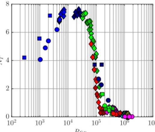
Even if transition reversal cannot be predicted with linear stability computations of the first and second modes, an approach combining the measurements and computations data will still be useful to evaluate where and when the transition process is no longer dominated by the second mode. Figure 2 presents a compilation of second-mode transitionN-factorsNT as a function of the nosetip Reynolds numberReRN for the Mach 6 experiments of Stetson [2] from Ref. [36] (diamonds), Mach 9 experiments of Stetson [2] from Ref. [35] (circles) and Mach 10 experiments of Marineau et al. [25] (squares). For values ofReRN below 1×10⁴,NT increases withReRN as a result of the increase in the unit Reynolds number. This behavior can be linked to an increase in the critical second-mode frequency fT,
which implies a lower tunnel noise content near fT. This effect, first discussed by Marineau et al. [25] and Marineau
[35], has recently been modeled by Balakumar and Chou [38] with direct numerical simulations (DNS) of the Tunnel 9 Mach 10 experiments. The approach includes the measured freestream noise spectrum and an empirical correlation (see Marineau et al. [25]) to determine the breakdown amplitude of the second mode. The sharp cone nosetip radius was not specified in either Stetson Mach 6 or Mach 9 experiments. To include these sharp cone data points in Fig. 2, the sharp nosetips were assumed to have the same radius as the sharp Tunnel 9 cone. A variation in the sharp cone nosetip radius does not change the trends, as it simply shifts the point left or right. ForReRN between approximately 4×10⁴and 1×10⁵, a steep decrease inNT withReRN is observed. Somewhere in this region, the transition process appears to not be dominated by second-mode amplification. Note that the departure from second-mode-dominated transition occurs prior to transition reversal. The decrease of NT with bluntness was discussed by Marineau [35] and attributed to a
decrease of the second-mode breakdown amplitudes and to an increase in the initial amplitudes. The decrease in the breakdown amplitudes is linked to the lower edge Mach number whereas the increase in the initial amplitudes is related to the decrease in the critical second-mode frequency fT as well as an increase in the receptivity coefficient withReRN. For these conditions, the measured and estimated transitionN-factors and the estimated receptivity coefficients are shown in Figs. 3(a) and 3(b), respectively.
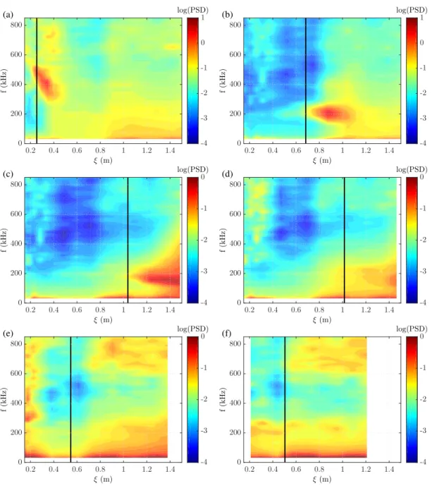
In contrast to Stetson’s blunt cone experiments, which measured just the transition location, Marineau et al. [25] also measured the boundary-layer instabilities by using a large number of high-frequency response pressure sensors (PCB®-132). These measurements captured the evolution of the pressure fluctuations over the surface of the cone. Figure 4 presents a map of the logarithm of the pressure power spectral density (log(PSD)) atRe∞≈17×106m−1for
102 103 104 105 106 107 ReRN 0 2 4 6 8 N T
Fig. 2 Computed second-mode N-factors at the experimental transition location (start of transition) as a function of the nosetip Reynolds number. The same symbols and colors as in Fig. 1 are used to indicate the nosetip radius. 104 105 ReRN 0 2 4 6 8 N T (a) 104 105 ReRN 10−1 100 101 102 CR /C R ,s (b)
Fig. 3 Effect of bluntness on (a) transitionN-factors and (b) receptivity for Stetson blunt cone experiments at Mach6. The same symbols and colors as in Fig. 1 are used to indicate the nosetip radius.
swallowed. This leads to a significant reduction of the edge Mach number compared to the sharp cone case. For the 5.1 mm nosetip in Fig. 4(b), the edge Mach number varies from 4.4 to 4.8 between the neutral point and the start of transition. The bluntness significantly delays the appearance of the second-mode waves and increases the distances over which growth and breakdown occur. As a result of these two factors, the transition location is moved further downstream on the blunt cone (from 0.25 m on the sharp cone to 0.68 m on the 5.1 mm cone, based on heat transfer measurements). In addition, the second-mode frequencies are significantly lower on the blunt cone due to the increased boundary-layer thickness. As the nosetip radius increases from 5.1 mm to 9.5 mm, the transition location moves further downstream and the unstable second-mode frequencies are further decreased. The increase from 9.5 mm to 12.7 mm has a minor effect on the transition location, which indicates that reversal is near. For the 12.7 mm nosetip, the start of transition occurs prior to significant growth of the second mode. This indicates that transition was not initiated by the second-mode instability. However, further downstream within the transitional region, the second-mode amplitudes keep increasing up to the downstream end of the cone. The 25.4 and 50.8 mm nosetips are in the reversal regime as the transition location has moved upstream compared to those at the smaller radii. In addition, transition occurs before the appearance of second-mode waves. This makes sense, as the edge Mach number at the start of transition for the 25.4 mm and 50.8 mm radii are 3.3 and 3.2 respectively, which are too low for second-mode growth. The results for 25.4 mm and 50.8 mm nosetips also reveal that the mechanism responsible for the transition reversal has a weak pressure signature, as no significant variation in the pressure PSD is found.
The use of fast-response heat flux sensors can help to characterize the transition mechanisms on blunt cones. For instance, time-resolved heat transfer measurements performed at Mach 9 by Zanchetta [39] in the Imperial College Gun Tunnel on a 5◦half-angle cone revealed that in the reversal regime, transitional events are formed in the
near-nose region and convect downstream. The formation frequency of the events was linked to the severity of the roughness environment. In certain cases, second-mode instability waves and these transition events were occurring concurrently; and the experiments indicated that the second mode was responsible for the completion of transition. Recent laser-induced-fluorescence-based (LIF) schlieren measurements from Grossir et al. [40] on a blunt 7◦half-angle
cone at Mach 11.9 in the von Karman Institute Longshot hypersonic wind-tunnel revealed disturbances with shapes quite different from the usual second-mode rope structures. The disturbances that extend above the edge of the boundary layer are seen in Fig. 5 for the 4.75 mm nosetip radius. These disturbances, that were not present on schlieren images for sharper cones, could be a manifestation of the blunt cone transition mechanism leading to the heat transfer fluctuation measured by Zanchetta [39].
In summary, the experimental and numerical studies agree that frustum transition in the reversal regime cannot be accounted for via linear, modal instability analysis. Furthermore, the experimental observations agree that frustum transition on large bluntness cones is highly sensitive to wall roughness and appears to be dominated by disturbances that originate in the vicinity of the nosetip. Therefore, roughness-induced transient growth emerges as the primary
0.2 0.4 0.6 0.8 1 1.2 1.4 ξ(m) 0 200 400 600 800 f (k H z) -4 -3 -2 -1 0 1 log(PSD) (a) 0.2 0.4 0.6 0.8 1 1.2 1.4 ξ(m) 0 200 400 600 800 f (k H z) -4 -3 -2 -1 0 1 log(PSD) (b) 0.2 0.4 0.6 0.8 1 1.2 1.4 ξ(m) 0 200 400 600 800 f (k H z) -4 -3 -2 -1 0 log(PSD) (c) 0.2 0.4 0.6 0.8 1 1.2 1.4 ξ(m) 0 200 400 600 800 f (k H z) -4 -3 -2 -1 0 log(PSD) (d) 0.2 0.4 0.6 0.8 1 1.2 1.4 ξ(m) 0 200 400 600 800 f (k H z) -4 -3 -2 -1 0 log(PSD) (e) 0.2 0.4 0.6 0.8 1 1.2 1.4 ξ(m) 0 200 400 600 800 f (k H z) -4 -3 -2 -1 0 log(PSD) (f)
Fig. 4 Contour map of the logarithm of the pressure power spectral density log(PSD) for cones with (a) RN =0.15mm (ξT =0.254m), (b)RN =5.1mm (ξT =0.683m), (c)RN =9.5mm (ξT =1.037m), (d)RN =12.7
mm (ξT =1.015m), (e)RN =25.4mm (ξT =0.546m), and (f)RN =50.8mm (ξT =0.504m), atRe∞ ≈17×106
m−1at Mach10in Tunnel9. The vertical, black line denotes the measured transition location.
Fig. 5 LIF-based schlieren flow visualization on4.75mm radius nosetip7◦half-angle cone in VKI atM∞=11.9
and Re∞ = 11.6×10⁶ m−1. Fields of view extend from x = 625mm until the end of the cone at 806mm.
candidate for the experimentally-observed trend in laminar-turbulent transition.
III. Transient Growth Analysis for Hypersonic Blunt Cones
This section presents the transient growth analysis of blunt circular cones with conditions selected to match a subset of the configurations from the experiments conducted by Stetson [2] in the Air Force Research Laboratory (AFRL) Mach 6 High Reynolds Number facility and by Marineau [25] in the Arnold Engineering Development Complex (AEDC) Tunnel 9 at Mach 10. Modal instability analysis for the AFRL configurations has been already performed by Jewell & Kimmel [36], and Marineau [25] has described similar analysis for the AEDC configurations. They found that both first-mode and Mack-mode waves were either damped or weakly unstable for the present configurations; and therefore, transition reversal cannot be predicted with the modal analysis. Another modal instability mechanism that might play a role in the transition reversal is the entropy-layer instability [41, 42]. However, although not shown here, our analysis did not revealed any substantially amplified entropy-layer modes for the configurations of interest. Therefore, the transient growth mechanism is investigated as a potential cause for the transition reversal. First, the basic state solutions are presented in subsection III.A. Second, the transient growth theory is briefly introduced in subsection III.B. Then, a detailed transient growth analysis of the selected blunt cones configurations is presented in subsection III.C.
A. Laminar Boundary Layer over Blunt Cones
The basic states used in the present analysis correspond to the laminar boundary layer flow over the selected blunt cone configurations. The laminar boundary layer flows were computed by Jewell & Kimmel [36] and Marineau [25] with reacting, axisymmetric Navier-Stokes equations on a structured grid. The solver was a version of the NASA data parallel-line relaxation (DPLR) code [43], that is included as part of the STABL-2D software suite, as described by Johnson [44] and Johnson et al. [45]. This flow solver employs a second-order-accurate finite-volume formulation. The inviscid fluxes are based on the modified Steger-Warming flux vector splitting method with a monotonic upstream-cente scheme for the conservation laws (MUSCL) limiter. The time integration method is the implicit, first-order data parallel line relaxation (DPLR) method. Additional details about the basic state solution and the grid convergence study are given by Jewell & Kimmel [36] for the AFRL configurations and by Marineau [25] for the AEDC configurations. 1. AFRL Configurations
The AFRL Mach 6 facility operates at stagnation pressures p0 from 700 to 2100 psi (4.83 to 14.5 MPa). The working fluid is air and is treated as ideal gas because of the relatively low temperature and pressure. The blunt cones used in the experiments have a half-angle of 8◦and a base radius of 2.0 in. (0.0508 m). A total of 196 experiments
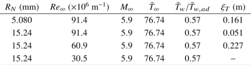
encompassing 108 unique conditions comprised the Stetson [2] Mach 6 results. Table 1 shows the details of the four configurations selected for the present analysis. The present analysis uses the 7◦half-angle variable-bluntness cone
that is currently used in the experiments in the AFRL Mach 6 facility. The thermal wall condition is isothermal with a constant wall temperature equal to ¯Tw =300.0 K.
Table 1 Details of the four AFRL configurations used in the present study. The wall temperature isT¯w =300
K. The measured transition locations,ξT, are extracted from Ref. [46].
RN (mm) Re∞(×106m−1) M∞ T¯∞ T¯w/T¯w,ad ξT (m)
5.080 91.4 5.9 76.74 0.57 0.161
15.24 91.4 5.9 76.74 0.57 0.051
15.24 60.9 5.9 76.74 0.57 0.227
15.24 30.5 5.9 76.74 0.57 −
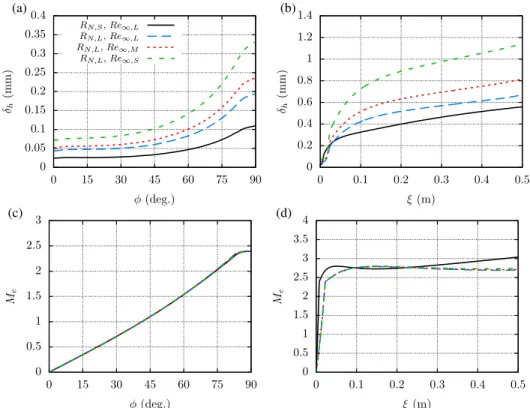
The streamwise evolution of the boundary layer thicknessδhand edge Mach numberMeis plotted in Fig. 6. The
boundary-layer edge,ηe=δh, is defined as the wall-normal position whereht/ht,∞=0.995, withhtdenoting the total
enthalpy, i.e.,ht=h+0.5(u¯2+v¯2+w¯2), wherehis the static enthalpy. The evolution of boundary layer thicknessδh
within the nose region and along the entire geometry is shown in Figs. 6(a) and 6(b), respectively. The boundary layer thickness is nearly constant from the stagnation point up toφ≈30◦, which is characteristic of stagnation boundary layer flow. Fromφ≈45◦, the boundary layer thickness grows monotonically up to the end of the cone, as shown in Fig. 6(b).
Figures 6(a) and 6(b) also show that the boundary layer thickness for the smaller nose radius (RN =9.53 mm) cone is
smaller than for the larger nose radius (RN =15.24 mm) cone with the same freestream conditions (Re∞=91.4×10⁶
m−1). Figures 6(c) and 6(d) show the evolution of the edge Mach number in the nose region and in the entire cone,
respectively. The edge Mach number is determined by inviscid theory to the leading order, and therefore, the evolution within the nose is nearly coincident for the four configurations (Fig. 6(c)). However, the edge Mach number evolution is clearly distinguishable from the smaller to the larger nose radius cases when it is plotted against the streamwise coordinate for the entire geometry (Fig. 6(d)). The sonic location, which coincides with the peak of the streamwise mass-flux within the nose [23, 24], is found atφ=41.4◦. The edge Mach number remains belowM
e=3 along the
entire geometry for the large nose radius cones and only becomes slightly larger thanMe=3 at the end of the cone for
the smaller nose radius case. 2. AEDC Configurations
The Air Force AEDC Hypervelocity Wind Tunnel No. 9 (Tunnel 9) is a hypersonic, nitrogen gas, blowdown wind tunnel with interchangeable nozzles that allow for testing at Mach numbers of 7, 8, 10, and 14 over a 0.177×10⁶m−1to 158.8×10⁶m−1unit Reynolds number range. A detailed description of the facility can be found in Ref. [25]. The blunt cones used in the experiments of Marineau et al. [25] had a base diameter of 15 in. (0.381 m) and interchangeable nose tips with radius of 0.152 mm to 50.80 mm. The test matrix for the 24 run test program is provided in Ref. [25]. The working fluid is nitrogen at a relatively low temperature and pressure. Thus, the effects of chemistry and molecular
0 0.05 0.1 0.15 0.2 0.25 0.3 0.35 0.4 0 15 30 45 60 75 90 δh (mm) φ(deg.) RN,S,Re∞,L RN,L,Re∞,L RN,L,Re∞,M RN,L,Re∞,S (a) 0 0.2 0.4 0.6 0.8 1 1.2 1.4 0 0.1 0.2 0.3 0.4 0.5 δh (mm) ξ(m) (b) 0 0.5 1 1.5 2 2.5 3 0 15 30 45 60 75 90 M e φ(deg.) (c) 0 0.5 1 1.5 2 2.5 3 3.5 4 0 0.1 0.2 0.3 0.4 0.5 M e ξ(m) (d)
Fig. 6 Streamwise evolution of (a,b) boundary layer thickness and (c,d) edge Mach number of the laminar boundary layer flows over the AFRL configurations. The legend refers toRN,S =5.08mm,RN,L =15.24mm,
Re∞,L =91.4×10⁶m−1,Re∞,M =60.9×10⁶m−1,Re∞,S =30.5×10⁶m−1.
vibration are omitted from the calculations. The viscosity law used is the Sutherland’s law and the heat conductivity is calculated using Eucken’s relation. Table 2 shows the details of the four configurations selected for the present analysis. The used thermal wall condition is isothermal with a constant wall temperature equal to ¯Tw =300.0 K. The
four configurations share a similar freestream unit Reynolds number ofRe∞ ≈17.5×10⁶m−1and a freestream Mach
number ofM∞ ≈9.78. The nose radius values varies fromRN =9.53 mm toRN =50.8 mm.
Table 2 Details of the four AEDC configurations used in the present study. The wall temperature isT¯w =300
K. The measured transition locations,ξT, are extracted from Ref. [25].
RN (mm) Re∞(m−1) M∞ T¯∞ T¯w/T¯w,ad ξT (m)
9.530 17.6×10⁶ 9.797 51.01 0.340 1.037 12.70 17.4×10⁶ 9.795 51.17 0.339 1.015 25.40 17.3×10⁶ 9.791 51.13 0.340 0.546 50.80 17.6×10⁶ 9.777 51.27 0.340 0.504
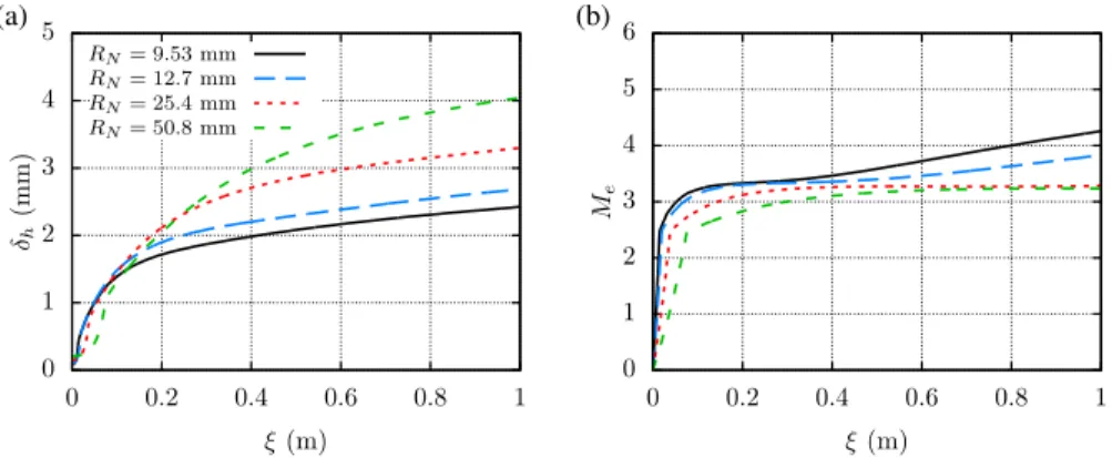
The boundary layer thicknessδh and edge Mach numberMefor the four configurations are plotted in Figs. 7(a) and
7(b), respectively. As observed in the comparison of the AFRL configurations of Fig. 6(b), despite the same freestream conditions, the boundary layer thickness in the frustum part of the cone is larger for larger nose radius values. Also, the edge Mach number is larger for the smaller nose radius cases, although remains smaller thanMe =4.5 for the four
0 1 2 3 4 5 0 0.2 0.4 0.6 0.8 1 δh (mm) ξ(m) RN= 9.53 mm RN= 12.7 mm RN= 25.4 mm RN= 50.8 mm (a) 0 1 2 3 4 5 6 0 0.2 0.4 0.6 0.8 1 M e ξ(m) (b)
Fig. 7 Streamwise evolution of (a) boundary layer thickness and (b) edge Mach number of the laminar boundary layer flows over the AEDC configurations.
configurations.
B. Transient Growth Theory
Transient growth analysis is performed using the linear PSE as explained in the literature [18, 23, 47–49]. The analysis focuses on stationary perturbations because, despite of the speed regime, they experience the largest transient growth. For completeness, the present section outlines the methodology, which bears strong similarities with the optimization approach based on the linearized boundary layer equations [17, 22, 50]. The advantage of the PSE-based formulation is that it is also applicable to more complex base flows where the flow evolves along the streamwise direction and the boundary layer approximation may not hold. The PSE approach can also be easily extended to unsteady disturbances. While infinite Reynolds number asymptotic results cannot be directly computed using this technique, good agreement is achieved between the two methodologies for incompressible and compressible regimes as shown by Paredes et al. [18].
In the PSE context, stationary perturbations have the form ˜ q(ξ, η, ζ)=qˆ(ξ, η)exp " i Z ξ ξ0 α(ξ 0)dξ0+ mζ−ωt !# +c.c., (1)
where c.c.denotes complex conjugate. The suitably nondimensionalized, orthogonal, curvilinear coordinate system
(ξ, η, ζ)denotes streamwise, wall-normal, and azimuthal coordinates and(u,v,w)represent the corresponding velocity
components. Density and temperature are denoted byρandT. The streamwise and azimuthal wavenumbers areα andm, respectively; andωis the angular frequency of the perturbation. The Cartesian coordinates are represented by
(x,y,z). The vector of perturbation fluid variables is ˜q(ξ, η, ζ,t)=(ρ,˜ u˜,v,˜ w,˜ T˜)Tand the vector of amplitude functions
is ˆq(ξ, η)=(ρ,ˆuˆ,v,ˆ w,ˆ Tˆ)T. The vector of basic state variables is ¯q(ξ, η)=(ρ,¯ u¯,v,¯ w,¯ T¯)T.
Upon introduction of the perturbation form (1) into the linearized NS equations together with the assumption of a slow streamwise dependence of the basic state and the amplitude functions, thus neglecting the viscous derivatives inξ,
the PSE are recovered as follows Lqˆ(ξ, η)= A+B ∂ ∂η +C ∂2 ∂η2 +D 1 h1 ∂ ∂ξ ! ˆ q(ξ, η)=0. (2)
The linear operatorsA,B,CandDare given by Pralits et al. [47] andh1 is the metric factor associated with the streamwise curvature. The system of Eqs. (2) is not fully parabolic due to the term∂pˆ/∂ξin the streamwise momentum equation [51–54]. However, for purely stationary disturbances (ω =0 andα =0), this term can be dropped from the equations as justified in Refs. [48, 55]. For nonstationary perturbations (ω,0), a commonly adopted solution is
to replace∂pˆ/∂ξbyΩP N S∂pˆ/∂ξ, whereΩP N Sis the Vigneron parameter [56–58]. This parameter was originally introduced for the integration of the parabolized Navier-Stokes equations (PNS) , and is determined by
ΩP N S =min(1,Mξ2), (3)
where Mξ is the local streamwise Mach number. The Vigneron approximation ensures numerical stability of the marching scheme by suppressing upstream influence within the solution. For locally supersonic flow, the equations are not altered becauseΩP N S =1. For a disturbance field withα,0, a portion of the elliptic behavior is absorbed in
the wave part via the term iαpˆand the residual upstream influence can be suppressed by choosing a sufficiently large marching step [53], without having to invoke the Vigneron approximation.
The optimal initial disturbance, ˜q0, is defined as the initial (i.e., inflow) condition atξ0that maximizes the objective function,J, which is defined as a measure of disturbance growth over a specified interval [ξ0, ξ1]. The definitions used in the present study correspond to the outlet energy gainJ=Goutand mean energy gainJ=Gmeanand are defined as
Gout = E(ξ1) E(ξ0), (4) Gmean 1 ξ1−ξ0 Rξ1 ξ0 E(ξ0)dξ0 E(ξ0) , (5)
whereEdenotes the energy norm of ˜q. The energy norm is defined as E(ξ)=
Z
ηqˆ(ξ, η)
HM
Eqˆ(ξ, η)h1h3dη, (6)
whereh3is the metric factor associated with the azimuthal curvature,MEis the energy weight matrix and the superscript
Hdenotes conjugate transpose. The selection ofJ=Goutcorresponds to the “outlet energy gain” that is commonly used in studies of the optimal-perturbation problem [22, 50]. The selection ofJ=Gmeandefines the “mean energy gain” and corresponds to the optimization of the mean energy. This latter definition accounts for a possible overshoot
in the disturbance energy evolution that are not accounted for by the former definition and is found to be present in hypersonic blunt forebodies [23, 24], as well as in the nosetip of blunt cones as documented in what follows.
The choice of the energy norm is known to influence the optimal initial perturbation as well as the magnitude of energy amplification [17, 49, 59]. Here, we use the positive-definite energy norm derived by Mack [60] and used by Hanifi et al. [61] for transient growth calculations, which is defined by
ME =diag " ¯ T(ξ, η) γρ¯(ξ, η)M2,ρ¯(ξ, η),ρ¯(ξ, η),ρ¯(ξ, η), ¯ ρ(ξ, η) γ(γ−1)T¯(ξ, η)M2 # . (7)
Additionally, the kinetic energy norm is also used for optimization in this paper. The kinetic energy of a perturbation is defined by K(ξ)= Z ηqˆ(ξ, η) HM Kqˆ(ξ, η)h1h3dη, (8) where MK =diag0,ρ¯(ξ, η),ρ¯(ξ, η),ρ¯(ξ, η),0. (9)
To differentiate when the total energy normEor the kinetic energy normKare used, a corresponding subscript is added to the energy gain, resulting in four options for the objective function:Gout
E ,GmeanE ,GoutK , andGmeanK . In the present
study, the transient growth amplification is also expressed in terms of the logarithmic amplification ratio, the so-called N-factor, based on the total energy norm, which is defined as
NE =12ln GoutE =− Z ξ ξ0 αi(ξ0)dξ0+1/2 lnfˆE(ξ)/ˆE(ξ0)g. (10)
Furthermore, the present study uses theN-factor based in other disturbance magnitude norms, as the kinetic energy,NK,
maximum temperature,NT, or maximum streamwise velocity,Nu. These definitions are equivalent to that of Eq. (10),
but with their respective norms.
The variational formulation of the problem to determine the maximum of the objective functional Jleads to an optimality system [18], which is solved in an iterative manner, starting from a random solution atξ0that must satisfy the boundary conditions. The PSE,Lq˜ =0, are used to integrate ˜qup toξ1, where the final optimality condition is used to obtain the initial condition for the backward adjoint PSE integration,L†q˜†=cmeanF(q˜), wherecmean =0 for
the outlet energy gain optimization andcmean =1 for the mean energy gain optimization, andF(q˜)is a function of
the direct solution [47]. Atξ0, the adjoint solution is used to calculate the new initial condition for the forward PSE integration with the initial optimality condition. The iterative procedure finishes when the value ofGhas converged up to a certain tolerance, which was set to 10−4in the present computations.
PSE along the wall-normal coordinate. The discretized PSE are integrated along the streamwise coordinate by using second-order backward differentiation. The number of discretization points in both directions was varied in selected cases to ensure convergence of the optimal gain predictions. The wall-normal direction was discretized usingNy =161,
with the nodes being clustered toward the wall [63]. No-slip, isothermal boundary conditions are used at the wall, i.e., ˆ
u=vˆ =wˆ =Tˆ =0. The amplitude functions are forced to decay at the farfield boundary by imposing the Dirichlet conditions ˆρ=uˆ=wˆ =Tˆ =0, unless otherwise stated. The farfield boundary coordinate is set just below the shock layer. Verification of the present optimal growth module against available transient growth results from the literature is shown in Ref. [18].
In what follows, we study the axisymmetric boundary layer over circular cones in hypersonic freestream flows. The freestream conditions and geometries are selected to match a subset of configurations used in the experiments conducted at AFRL [2, 36] and at AEDC [25]. For this problem, the computational coordinates,(ξ, η, ζ), are defined as
an orthogonal body-fitted coordinate system. The metric factors are defined as
h1 = 1+κη, (11)
h3 = rb+ηcos(θ), (12)
whereκdenotes the streamwise curvature,rbis the local radius, andθis the local half-angle along the axisymmetric
surface, i.e., sin(θ)=drb/dξ. For our study, the half angle,θ, is 7◦andκ =0 in the frustum region. The end of the
nose and beginning of the frustum is denoted as the juncture location that is defined asξj =RNπ/2. The streamwise
coordinate within the nosetip region is represented by an angular coordinate defined asφ=ξ/RN. The nosetip Reynolds
number, ReRN = ρ¯∞u¯∞RN/µ∞ is used to scale the energy gain. The length scale LRN = RN/ p
ReRN is used to normalize the spanwise disturbance wavelength defined asλ=2πrb/m.
C. Transient Growth Results
For a nonselfsimilar boundary layer such as the boundary layer over blunt cones, both the initial and final locations must be varied in order to obtain the overall picture of the optimal growth characteristics [23]. A special feature of the transient growth analysis for the blunt cones of interest is that the results naturally split into two parts, one that deals with transient growth intervals that are limited to the nose region, where the results are expected to resemble those for the hemisphere forebody reported by Paredes et al. [23], and a second one that deals with transient growth intervals that extend into the frustum region, where transition is observed in the experiments. Detailed transient growth results are first presented for the AFRL configurations in subsections III.C.1 and III.C.2. Because stationary disturbances usually yield the highest transient growth overall, a majority of the analysis in section III is focused on the zero frequency case. However, motivated by the findings of Cook et al. [64], who performed a resolvent analysis of a similar blunt cone
0 15 30 45 60 75 90 φ0(deg.) 0 15 30 45 60 75 90 φ1 (d eg .) 50 100 150 200 250 Gmean E (a) 0 15 30 45 60 75 90 φ0(deg.) 0 15 30 45 60 75 90 φ1 (d eg .) 10 20 30 40 50 60 GmeanK (b)
Fig. 8 Contours of (a) optimal mean total energy gainGmeanE and (b) optimal mean kinetic energy gainGmeanK within the nose region of theRN =15.24mm andRe∞=91.4×10⁶m−1case. The solid line in the contour plot
indicates the value ofφ1corresponding to maximum energy gain for a givenφ0.
configuration at hypersonic conditions and reported significant nonmodal growth of planar, traveling waves inside the entropy layer, the transient growth analysis is extended to traveling disturbances in subsection III.C.3. Finally, a brief summary of results is presented for the AEDC configurations in subsection III.C.4.
1. Transient Growth Interval within the Nose Region
Herein, transient growth results with initial and final disturbance locations within the nose region for the AFRL configurations introduced in Table 1 are investigated. The optimal mean total energy gain (GmeanE ) and optimal mean kinetic energy gain (GmeanK ) for theRN =15.24 mm andRe∞=91.4×10⁶m−1case are plotted in Figs. 8(a) and 8(b),
respectively. Figure 8(a) shows that the highest total energy gain occurs for relatively short optimization intervals in the vicinity of the stagnation point, as indicated by the black line nearly parallel to the lower boundary of the plot. However, the kinetic energy budget for these perturbations initiated near the stagnation point is rather small. This fact is confirmed by the optimal mean kinetic energy gain (GmeanK ) plot of Fig. 8(b). The optimal kinetic energy gain exhibits a maximum in the interior of the domain atφ0=42.4◦that nearly coincides with the sonic location,φ
M e=1=41.4◦. These results
indicate the same features as the results reported by Paredes et al. [23] for a hypersonic hemisphere forebody. The optimal growth results for a specified inflow locationξ0of the flow are characterized in terms of the combination of azimuthal wavenumbermand outflow locationξ1that lead to the maximum value of the energy gain. Thus, the effect of nosetip radiusRN on the maximum value of the optimal energy gain, optimal wavenumber, and optimal
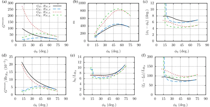
growth interval, is analyzed next. Figure 9 shows the optimal total and kinetic energy gains as a function of the inflow location (Figs. 9(a) and 9(d)), as well as the corresponding azimuthal wavenumber (Figs. 9(b) and 9(e)) and the optimal growth interval (Figs. 9(c) and 9(f)). Results are shown for theRN =5.08 mm andRN =15.24 mm cones at the same
0 50 100 150 200 250 300 0 15 30 45 60 75 90 G mean φ0(deg.) GE,RN,S GK,RN,S GE,RN,L GK,RN,L (a) 0 200 400 600 800 1000 0 15 30 45 60 75 90 m φ0(deg.) (b) 0 2 4 6 8 10 12 0 15 30 45 60 75 90 ( φ1 − φ0 ) (deg.) φ0(deg.) (c) 0 5 10 15 20 25 0 15 30 45 60 75 90 G mean /R eR N (10 − 5) φ0(deg.) (d) 0 2 4 6 8 10 12 14 0 15 30 45 60 75 90 λ0 /L RN φ0(deg.) (e) 0 50 100 150 200 0 15 30 45 60 75 90 ( ξ1 − ξ0 ) /L R N φ0(deg.) (f)
Fig. 9 (a,d) Optimal mean energy gain and corresponding (b,e) azimuthal wavenumber and (c,f) optimization interval within the nose region for RN,S = 5.08 mm and RN,L = 15.24 mm cones at same freestream unit
Reynolds number,Re∞=91.4×10⁶m−1.
gains are larger for the larger nose radius, although as shown in Fig. 9(d), the scaling is not perfectly linear because, as indicated by Paredes et al. [24], small deviations from the linear scaling occur as a result of the differences in the ratio of boundary-layer thickness to the radius of the surface curvature. Figure 9(b) shows that the optimal azimuthal wavenumber is nearly twice as large for the larger nose radius cone in comparison with the case of the smaller nose radius. The scaling of the initial disturbance wavelength withLRN plotted in Fig. 9(e) shows a reasonable scaling with the boundary layer thickness. On the other side, the optimal growth interval plotted in Fig. 9(c) does not scale withLRN (orRN) as shown in Fig. 9(f), presumably because the ratio of boundary-layer thickness to the radius of the surface
curvature plays an important role for this parameter. 2. Transient Growth along the Frustum Region
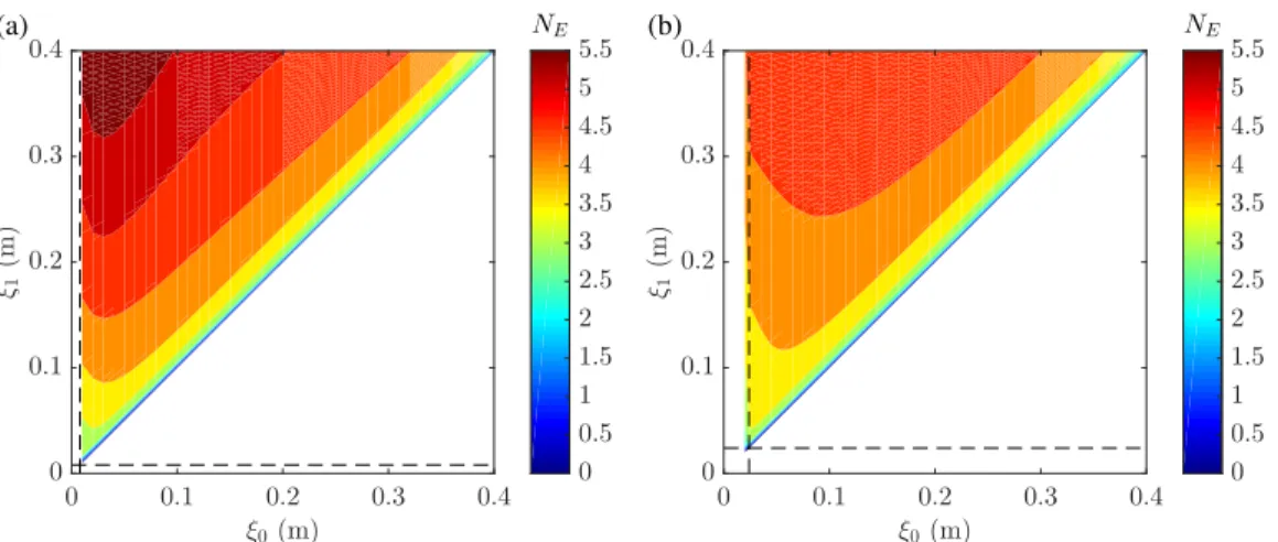
Next, transient growth across spatial intervals that extend into the frustum region is studied in detail for the AFRL configurations. In this case, we find it more convenient to plot the transient growth amplification in terms of theN-factor based on the total energy norm defined in Eq. (10). Figures 10(a) shows theN-factor contours for initial and final locations on the frustum for theRN =5.08 mm AFRL cone atRe∞=91.4×10⁶m−1. Similar results for the larger
nose radius,RN =15.24 mm, are shown in Fig. 10(b). TheN-factor values are larger for the smaller nose radius cone
except for initial and final locations near the juncture of the cone, i.e., beginning of the frustum. TheNEvalues are
larger than 5.5 in the studied range of parameters for the smaller nose radius case (Fig. 10(a)). For the larger nose radius case, theNE values are larger than 4.5 in the range ofξ0andξ1values studied here, although theNE=3.5 value is
0 0.1 0.2 0.3 0.4 ξ0(m) 0 0.1 0.2 0.3 0.4 ξ1 (m ) 0 0.5 1 1.5 2 2.5 3 3.5 4 4.5 5 5.5 NE (a) 0 0.1 0.2 0.3 0.4 ξ0(m) 0 0.1 0.2 0.3 0.4 ξ1 (m ) 0 0.5 1 1.5 2 2.5 3 3.5 4 4.5 5 5.5 NE (b)
Fig. 10 Contours ofN-factor values defined asNE =1/2ln(GoutE )in the frustum region of the (a)RN =5.08
mm and (b)RN =15.24mm cones. The juncture locationξjis marked with a vertical and a horizontal dashed
line. The freestream unit Reynolds number isRe∞=91.4×10⁶m−1.
reached at smaller values ofξ1than for the smaller radius case when the initial disturbance location is near the juncture locationξ0 ≈ξj.
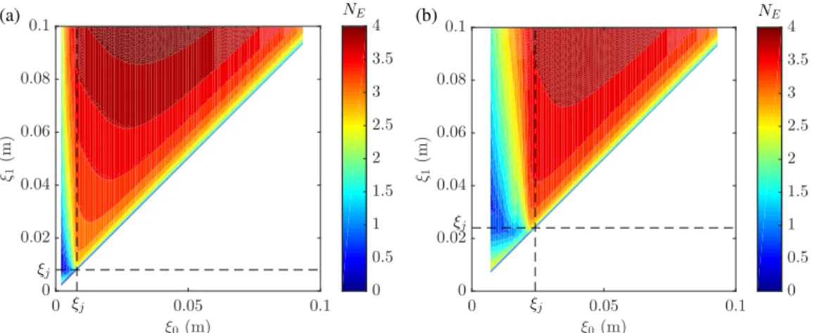
Figures 11(a) and 11(b) show a magnified view of theN-factor contours from Figs. 10(a) and 10(b), respectively, for initial and final locations in the vicinity of the juncture between the nose and the frustum of the cone. Both figures show different behavior of the transient growth amplification for disturbances initiated within the nose region (ξ0 < ξj) and
those that are initiated downstream of the juncture location (ξ0 ≥ξj). The disturbances initiated in the nose have a maximum for very short optimal growth intervals, as previously shown in Fig. 9. For larger optimal growth intervals, the transient growth amplification first decreases and then increases again forξ1 > ξj. On the other side, disturbances
initiated downstream of the nose (ξ0 ≥ξj) experience a monotonic increase in energy gain factor asξ1is increased. Remarkably, disturbances initiated in the vicinity of the juncture location (ξ0 ≈ξj) experience a quite rapid growth for the blunter case and short transient growth intervals (Fig. 11(b)), resulting in relatively significant values ofNEjust
downstream of the juncture location.
The AFRL experiments investigated the effect of an azimuthally-periodic array of roughness elements mounted near the sonic point atφ=45◦. To help gain some insight into the role of transient growth as a mechanism for roughness
effects, we next examine the details of transient growth disturbances initiated in the nose region atφ0 =ξ0/RN =45◦,
which coincides with the location of the roughness array. A description of the experimental findings is deferred to section IV. Figure 12 shows the mean total energy gain and corresponding azimuthal wavenumber as a function of the optimal growth interval,∆ξ=ξ1−ξ0, for the four AFRL configurations shown in Table 1. Figure 12(a) shows that the trend previously observed forξ0 < ξj atRe∞ =91.4×10⁶m−1(Fig. 11(b)) also applies at other Reynolds
numbers. Specifically, the optimal energy gain has a maximum immediately downstream of the inflow station and then decays up to a plateau zone before increasing again for longer transient growth intervals. For the same freestream unit
ξj ξj 0 0.05 0.1 ξ0(m) 0 0.02 0.04 0.06 0.08 0.1 ξ1 (m ) 0 0.5 1 1.5 2 2.5 3 3.5 4 NE (a) ξj ξj 0 0.05 0.1 ξ0(m) 0 0.02 0.04 0.06 0.08 0.1 ξ1 (m ) 0 0.5 1 1.5 2 2.5 3 3.5 4 NE (b)
Fig. 11 Contours of N-factor values defined as NE = 1/2ln(GoutE ) in the vicinity of the nose region of the
(a) RN = 5.08mm and (b) RN =15.24mm cones. The juncture locationξj is marked with a vertical and a
horizontal dashed line. The freestream unit Reynolds number isRe∞=91.4×10⁶m−1.
Reynolds number, the initial peak in optimal energy gain is larger for the larger nose radius cone than for the smaller nose radius case, but this situation is reversed for larger optimal growth intervals (∆ξ >0.02 m). Figure 12(b) shows that the three regions translate into a discontinuous evolution of the corresponding azimuthal wavenumber. The scaling of the optimal mean total energy gain withReRN (Fig. 12(c)) and of the corresponding initial azimuthal wavelength withLRN (Fig. 12(d)) is reasonable for the cases with same nose radiusRN =15.24 mm and different freestream unit Reynolds numbers, but not for the smaller nose radius case (RN =5.08 mm) and outside the nose region.
Figure 13 shows further details of the transient growth disturbances initiated in the nose atφ0 =45◦for the blunter
cone at the highestRe∞configuration (RN =15.24 mm andRe∞ =91.4×10⁶m−1). Three cases based on the trends
observed in Fig. 12 are plotted; namely, (A)∆ξ=0.0030 m andm=420; (B)∆ξ=0.023 m andm=150; and (C) ∆ξ=0.091 m andm=80. The case (A) corresponds to the first peak in mean energy gain that is larger for the larger nose radius cone (Fig. 12(a)). The evolution of the disturbance amplitude√E/E0for the case (A) shows a rapid rise to its peak value within a rather short distance from the initial disturbance location and a slower subsequent decay with values lower than 1 for streamwise locations in the frustum region. The initial optimal perturbation plotted in Fig. 13 is mostly contained within the boundary layer thickness; and hence, such initial disturbance profiles are better suited for excitation via surface roughness than some other cases where the initial profiles extend well outside of the boundary layer. The disturbance amplitude evolution of the case (B) has a smaller initial peak and then remains below 6 along the streamwise domain plotted in Fig. 13. The initial optimal perturbation associated with this case (B) is similar to that in case (A), but the peaks of the perturbation variables are located somewhat farther from the wall, which presumably makes this perturbation less likely to be excited via surface roughness. The energy gain evolution for case (C) (∆ξ=0.091 m,m=80) shows rather small disturbance amplification near the inflow location and then a monotonic amplification up toξ=0.2 m. Figure 13 shows that the optimal initial perturbation shape in case (C) is more complex
0 20 40 60 80 100 0 0.02 0.04 0.06 0.08 0.1 G mean E ξ1−ξ0(m) RN,S,Re∞,L RN,L,Re∞,L RN,L,Re∞,M RN,L,Re∞,S (a) 0 100 200 300 400 500 600 700 800 0 0.02 0.04 0.06 0.08 0.1 m ξ1−ξ0(m) (b) 0 2 4 6 8 10 12 14 16 0 0.02 0.04 0.06 0.08 0.1 G mean E /R eR N (10 − 5) ξ1−ξ0(m) (c) 0 20 40 60 80 100 120 0 0.02 0.04 0.06 0.08 0.1 λ0 /L R N ξ1−ξ0(m) (d)
Fig. 12 (a,c) Optimal mean energy gain and corresponding (b,d) azimuthal wavenumber with initial distur-bance locationφ0 =45◦ (ξ0 =0.04m for the RN =5.08mm cone andξ0 =0.012m for theRN =15.24mm
cone). The legend refers toRN,S =5.08mm,RN,L=15.24mm,Re∞,L =91.4×10⁶ m−1,Re∞,M =60.9×10⁶
0 5 10 15 20 25 0 0.05 0.1 0.15 0.2 p E /E 0 ξ(m) (A) (B) (C) 0 0.1 0.2 0.3 −1 0 1 η (mm) ˆ q0(10−2) ˆ u ˆ v ˆ w ˆ T ˆ ρ (A) 0 0.1 0.2 0.3 −1 0 1 η (mm) ˆ q0(10−2) (B) 0 0.1 0.2 0.3 −1 0 1 η (mm) ˆ q0(10−2) (C)
Fig. 13 Evolution of the disturbance amplitude√E/E0and corresponding initial optimal perturbations for the RN =15.24mm andRe∞ =91.4×10⁶m−1 configuration. The selected optimization intervals and azimuthal
wavenumbers are (A)∆ξ=0.0030m andm=420; (B)∆ξ=0.023m andm=150; and (C)∆ξ=0.091m and m=80. The initial disturbance location is set at the nosetip atφ0=45◦that corresponds toξ
0 =0.012m. The horizontal, dash-double dot lines indicates the edge of the boundary layer based on total enthalpy,η=δh.
than that for cases (A) and (B), because the perturbation profiles for wall-normal and spanwise velocity components have two and three peaks instead of one and two peaks, respectively. Also, the perturbation profiles have a larger wall-normal extension and the peaks of these profiles are located farther from the wall. In summary, the results shown in Fig. 13 indicate that roughness-induced perturbations atφ0=45◦can experience transient growth in a short interval within the
nose region. The transient growth streaks can lead to the onset of nonstationary streak instabilities that typically amplify rather rapidly and induce transition shortly after their onset; see Refs. [65–70] for details on secondary instability of streaks in high-speed boundary layers.
Previously, disturbances initiated in the vicinity of the juncture location,ξj =RNπ/2, were found to experience
a larger growth for the larger nose radius cone and relatively short transient growth intervals. This finding is further investigated here. Figure 14 shows the mean gain in total energy and corresponding azimuthal wavenumber as a function of the optimal growth interval,∆ξ=ξ1−ξ0, for the four AFRL configurations shown in Table 1. Figure 14(a) shows in details that the trend observed in Fig. 11(b) is forRe∞=91.4×10⁶m−1is also found at other Reynolds numbers.
Specifically, the energy gain has a monotonic increasing evolution as∆ξis increased, and the energy gain is larger for larger nose radius for relatively short optimization intervals (∆ξ <0.13 m). The difference between the energy gain values for the two nose radii (RN =5.08 and 15.24 mm) and same freestream unit Reynolds number (Re∞=91.4×10⁶
m−1) reaches about a factor of 2 for∆ξ=0.05 m. The azimuthal wavenumbers associated with the optimal energy gain
values of Fig. 14(a) are shown in Fig. 14(b). The azimuthal wavenumber quickly decreases and as the length of the transient growth interval increases, albeit at a decreasing rate. Compared to the large bluntness cases (RN =15.24
mm), the smaller radius case (RN =5.08 mm,Re∞=91.4×10⁶m−1) shows a notable, different behavior of both the
optimal energy gain and the associated azimuthal wavenumbers. This difference is clearly observed in the scaled mean energy gain and scaled initial wavelength plotted in Figs. 14(c) and 14(d), respectively. The large nose radius cases
0 0.5 1 1.5 2 2.5 3 3.5 4 0 0.05 0.1 0.15 0.2 0.25 G mean E (10 3) ξ1−ξ0(m) RN,S,Re∞,L RN,L,Re∞,L RN,L,Re∞,M RN,L,Re∞,S (a) 0 100 200 300 400 500 0 0.05 0.1 0.15 0.2 0.25 m ξ1−ξ0(m) (b) 0 5 10 15 20 25 30 35 40 0 0.05 0.1 0.15 0.2 0.25 G mean E /R eR N (10 − 4) ξ1−ξ0(m) (c) 0 20 40 60 80 100 0 0.05 0.1 0.15 0.2 0.25 λ0 /L RN ξ1−ξ0(m) (d)
Fig. 14 (a,c) Optimal mean energy gain and corresponding (b,d) azimuthal wavenumber with initial distur-bance location set in the juncture at ξ0 = ξj = RNπ/2(ξ0 = 0.008m for RN =5.08mm and ξ0 = 0.024m for RN = 15.24 mm.) The legend refers to RN,S = 5.08 mm, RN,L = 15.24 mm, Re∞,L = 91.4×10⁶ m−1,
Re∞,M =60.9×10⁶m−1,Re∞,S =30.5×10⁶m−1.
(RN =15.24 mm) show a perfect scaling of both properties as the unit Reynolds number is varied, but the scaled values
corresponding to the small radius case (RN =5.08 mm) are clearly different from the blunt nose cases. The reason for
this poor scaling of the transient growth parameters with nose radius could be due to the lack of selfsimilarity of the boundary layer profiles near the nose.
Figure 15 shows further details of the transient growth disturbances initiated at the juncture location for the RN =15.24 mm andRe∞=91.4×10⁶m−1configuration. The three cases shown in Fig. 15 for theRN =15.24 mm
case correspond to (A)∆ξ=0.0295 m andm=200; (B)∆ξ=0.0668 m andm=150; and (C)∆ξ=0.2066 m and m=110. Figure 15 shows that the peak in disturbance amplitude moves slightly downstream as the optimal growth interval becomes longer from case (A) to case (C). This peak is barely reached at the end of the cone length for the case (C). The optimal initial perturbations associated with the three cases are plotted in Fig. 15. The wall-normal extension and the peaks of these profiles are located closer to the wall for shorter optimal growth intervals, which makes them more closely related to roughness-induced perturbations. A wall-mounted device is not expected to generate a perturbation with the wall-normal extension of the optimal perturbation corresponding to case (C). Although not shown here, equivalent results for the small radius case (RN =5.08 mm,Re∞=91.4×10⁶m−1) and an optimal growth interval
0 20 40 60 80 100 0 0.1 0.2 0.3 0.4 0.5 p E /E 0 ξ(m) (A) (B) (C) 0 0.1 0.2 0.3 0.4 0.5 −1 0 1 η (mm) ˆ q0(10−2) 10׈u ˆ v ˆ w 10×Tˆ 10×ρˆ (A) 0 0.1 0.2 0.3 0.4 0.5 −1 0 1 η (mm) ˆ q0(10−2) (B) 0 0.1 0.2 0.3 0.4 0.5 −1 0 1 η (mm) ˆ q0(10−2) (C)
Fig. 15 Evolution of the disturbance amplitude√E/E0and corresponding initial optimal perturbations for the RN =15.24mm andRe∞ =91.4×10⁶m−1 configuration. The selected optimization intervals and azimuthal
wavenumbers are (A)∆ξ=0.0295m andm=200; (B)∆ξ=0.0668m andm=150; and (C)∆ξ=0.2066m and m=110. The initial disturbance location is set at the junctureξ0 =ξj that corresponds toξ0 =0.024m. The
horizontal, dash-double dot lines indicates the edge of the boundary layer based on total enthalpy,η=δh.
to the large radius cone (RN =15.24 mm,Re∞=91.4×10⁶m−1) plotted in Fig. 15. Similar to results for disturbances
initiated near the sonic location, these results withξ0=ξj indicate that roughness-induced perturbations can experience
greater transient growth for larger nosetip bluntness at the same freestream conditions. Therefore, transition onset could be driven by roughness-induced transient growth if the streak amplitude required for streak instabilities is reached. 3. Transient Growth of Traveling Disturbances along the Frustum Region
Next, we present salient findings pertaining to the nonmodal growth of traveling disturbances over the frustum region of the AFRL cone for the case ofRN =5.08 mm andRe∞=91.4×10⁶m−1. A detailed parameter study of
traveling mode disturbances is deferred to Paredes et al. [71]. The procedure used for the transient growth analysis of traveling disturbances is the same as that used earlier for the stationary disturbances withα=0, except with the addition of the streamwise pressure gradient term that is approximated with Eq. (3) based on the work by Vigneron et al. [56] for PNS equations. For the results presented herein, we confine our attention to a transient growth interval of
(ξ0;ξ1)=(0.04; 0.161)m. The selected outflow location corresponds to the transition location measured by Jewell et
al. [46] as indicated in Table 1, whereas the inflow location was chosen on the basis of a parameter study, which showed that the maximum energy gain occurs forξ0 =0.04 m for most combinations of frequency and azimuthal wavenumber. Figure 16 shows the contours of theN-factor based on the total energy gain,NE, as a function of the frequency,
F, and azimuthal wavenumber,m. The outlet energy gain is selected as the objective function for the optimal growth analysis. One may observe that the maximum energy gain ofNE=4.59 is achieved by a stationary, three-dimensional
perturbation withF =0.0 kHz and m=82. This stationary disturbance is the same as that studied previously in section III.C.2. Additionally, Fig. 16 shows a second, local maximum (NE =3.27) in theN-factor contours for planar