Using mutual information to select test suites in a black-box framework

USING MUTUAL INFORMATION TO SELECT TEST

SUITES IN A BLACK-BOX FRAMEWORK

ALFREDO IBIAS MARTÍNEZ

MÁSTER EN MÉTODOS FORMALES EN INGENIERÍA INFORMÁTICA FACULTAD DE INFORMÁTICA

UNIVERSIDAD COMPLUTENSE DE MADRID

Trabajo Fin de Máster en Métodos Formales en Ingeniería Informática Junio 2019 Director: Manuel Núñez Convocatoria: Junio-Julio 2019 Calificación: Sobresaliente - 10

Autorización de difusión

Alfredo Ibias Martínez

Junio 2019

El abajo firmante, matriculado en el Máster en Métodos Formales en Ingeniería Infor-mática de la Facultad de InforInfor-mática, autoriza a la Universidad Complutense de Madrid (UCM) a difundir y utilizar con fines académicos, no comerciales y mencionando expresa-mente a su autor el presente Trabajo Fin de Máster: “Using mutual information to select test suites in a black-box framework”, realizado durante el curso académico 2018-2019 bajo la dirección de Manuel Núñez en el Departamento de Sistemas Informáticos y Computación, y a la Biblioteca de la UCM a depositarlo en el Archivo Institucional E-Prints Complutense con el objeto de incrementar la difusión, uso e impacto del trabajo en Internet y garantizar su preservación y acceso a largo plazo.

Resumen en castellano

Lainformación mutua es una medida usada en Teoría de la Información para cuantificar la cantidad de similaridad entre dos variables aleatorias que actúan sobre dos conjuntos. En este trabajo, adaptamos este concepto y mostramos cómo puede usarse para seleccionar un buen conjunto de tests, en un escenario de caja negra y usando el enfoque de maxi-mizar la diversidad. Aportamos evidencias experimentales para mostrar la utilidad de la medida propuesta. También mostramos que el tiempo necesario para calcular la medida es despreciable cuando lo comparamos con el tiempo necesario para aplicar tests adicionales. Finalmente, comparamos nuestra medida con las mejores medidas disponibles para prior-ización de tests y mostramos que nuestra propuesta las supera.

Además, en este trabajo presentamos un enfoque basado en Programación Genética, respaldado por una herramienta, para generar conjuntos de tests utilizando medidas basadas en la Teoría de la Información.

Palabras clave

Abstract

Mutual Information is an information theoretic measure designed to quantify the amount of similarity between two random variables ranging over two sets. In this paper, we adapt this concept and show how it can be used to select agood test suite, in a black-box scenario and following a maximize diversity approach. We provide experimental evidence to show the usefulness of the measure. We also show that the time needed to compute the measure is negligible when compared to the time needed to apply extra testing. Finally, we compare our measure with current test prioritization measures and show that our proposal outperforms them.

As a side result, in this thesis we present a Genetic Programming approach, fully sup-ported by a tool, to generate test suites using Information Theory based measures.

Keywords

Contents

4.4 Research questions answers . . . 38

4.5 A tool to compare different measures . . . 43

4.5.1 The Genetic Programming algorithm . . . 43

4.5.2 The tool . . . 48

5 Threats to validity 53

6 Final discussion: alternative definitions 55

7 Conclusions 61

Acknowledgements

I would like to thank my thesis supervisor for his invaluable help and advice and for all the work he did to help me during this thesis. I would also like to thank Professor Robert M. Hierons and David Griñan for their support and their revisions of the work. Finally, I would like to thank my family for his moral and economical support.

Dedication

Chapter 1

Introduction

Software testing [3, 36] is the main technique to validate complex systems with the goal of increasing their reliability. Traditionally, software testing has been a mainly manual process, strongly depending on the knowledge of the specific group of testers. However, for more than 20 years, it has been shown that testing can have a formal basis [19]. Actually, formal testing is currently an active research area [6, 9, 24] and the existence of several tools that support formal testing has led to the recognition that the combination of formal methods and testing strongly facilitates test automation [41].

One of the problems that testing activities confront is that, being a time/resources con-sumption part of the software development process, an appropriate testing process usually needs more time than the available one (mainly due to budget constraints because testing can cost more than 50% of the development budget [36]). Therefore, it is very important to define methodologies that reduce the time without notably decreasing the confidence on the reliability of the system. A good starting point to diminish the time devoted to testing is to reduce the number of tests that we apply to the System Under Test (SUT). In fact,

the possible number of tests needed to exhaustively test even the simplest systems is exor-bitant. For example, exhaustive testing of a black-box implementation of a method adding two numbers on a 32-bit machine needs around 8·1028 _{tests. Therefore, it is imperative} to select a reduced number of tests having good capabilities to detect faults in the SUT.

choosing among different test suites, with the same size, the one that might have a greater expectation of finding faults.

We work within a black-box framework, that is, the SUT is a black-box from which we

only assume that we know its alphabet. Therefore, we cannot make any assumptions about the internal structure of theSUT. A side-effect of this setting is that we will not be sure that

we are totally covering theSUTbecause we cannot know whether a certain internal state has

been reached, despite the length of the applied tests. On the contrary, we have complete access to the specification of the system that we want to build. In order to simplify the presentation, we will assume that the specification of a system is given by a Finite State Machine (FSM) but our work can be easily adapted to deal with other state-based formalisms. In this context, it makes perfect sense to choose between different finite test suites, but with the same number of inputs, which one we apply to the SUT. We will define an information

theoretic measure to perform this choice. Specifically, we will define a notion inspired by

mutual information [42] and use it to compute, among different test suites, the one with the lowest mutual information. Our intended goal is to indirectlymaximize diversity because it has been widely recognised that diversity has a strong impact on test quality [8,17,21,22]. In order to assess the validity of our approach we performed experiments using the following approach. We started with a specification that we used with two goals:

• Derivation of test suites. We randomly traverse the specification to generate test suites. As usual when testing from FSMs, a test will be a sequence of (input, output)

pairs.

• Generation of mutants. We will generate mutants from the specification. The rationale is that a test suite is better than another one if the first one kills more mutants than the second one. In this setting, we do not need to worry about the problem of equivalent mutants [29,32] because we will compare numbers of killed mutants: none of the test suites will kill equivalent mutants.

Next we describe our scenario, which we consider to be highly realistic in practical terms. We consider that our testing process has the following properties:

• It is easy to generate different test suites.

• It is relatively easy to select which one of them is the best one (where being the best is equivalent to get the best score in a given measure).

• It is expensive to apply a lot of tests (so that we cannot perform exhaustive testing). For our experiments, we fix the size of the test suites, the number of generated mutants and the size of the FSMs (number of states, size of alphabet, outgoing transitions, etc...).

Then, we generate test suites and compare their capabilities to detect mutants versus our measure score and show that there is a correlation.

Summarizing the results of our experiments, we repeated the process 50 times and we obtained that our method chooses the test suite that kills more mutants around 75% of the times. Moreover, we obtained a correlation of our measure with the mutation score of −0.650256. These results allow us to claim that there is a relevant correlation between our measure and the ability to kill mutants. In addition, we provide a cheap method (in terms of computational power) to choose between test suites. Note that if the application of test suites were cheap (for example, in terms of time), then it would be better to apply all the available tests. However, the application of tests can be time intensive (in addition to the proper monetary costs). In this case, we really need to choose a reduced number of test. Our work provides a method that almost 75% of the times chooses the a priori best test suite. Moreover, our experiments show that the time needed to compute our measure is negligible when compared to the time needed to apply a single test suite. Finally, our experiments show that our measure gets better results than the current best information theory based measures.

Information Theory has been already used for testing [7,11,34,37–39,44]. In particular, the problem of choosing among different test suites has been addressed before [16, 17, 20]

and different test prioritization techniques have been compared [23].

We have already used Information Theory for black-box testing in order to detect failed error propagation in the execution of a test [26]. However, to the best of our knowledge, this is the first work where a measure inspired in Information Theory is specifically made to choose between test suites in a black-box testing framework.1 _{Also, the measure proposed in}

this work improves the results obtained by previously proposed test prioritization measures. The rest of the thesis is structured as follows. In Section2we review some basic concepts and notation that we will use along the thesis. In Section 3 we formally define our measure and show some simple examples to motivate the usefulness of its current definition. In Section 4 we report on our experiments. In Section 5 we analyse some threats to the validity of our results. In Section 6 we discuss some decisions that we took during the research presented in this thesis. Finally, in Section 7 we give our conclusions and some lines for future work.

1

Some work has somehow adapted measures specifically designed in white-box testing to a black-box testing setting [23].

Chapter 2

Preliminaries

In this thesis, systems will be modelled as Finite State Machines (FSMs). In order to define

anFSM, we first need to set some previous notations. Given a setA, we letA∗ _{denote the set}

of finite sequences of elements of A; ǫ∈A∗ _{denotes the empty sequence. We let A}+ _denote the set of non-empty sequences of elements of A. We let |A| denote the cardinal of set A. Given a sequence σ∈A∗_{, we have that|σ|denotes its length. Given a sequenceσ ∈A}∗ _and

a ∈A, we have thatσa denotes the sequence σ followed by a and aσ denotes the sequence

σ preceded bya.

Throughout this thesis we let I be the set of input actions and O be the set of output actions. It is important to differentiate between input actions and inputsof the system. In our context an input of a system will be a non-empty sequence of input actions, that is, an element of I+

(similarly for outputs and output actions).

An FSM is a (finite) labelled transition system in which transitions are labelled by an

input/output pair. We use this formalism to define specifications.

Definition 1. We say that M = (Q, qin, I, O, T)is a Finite State Machine (FSM), where Q

is a finite set of states, qin∈Q is the initial state, I is a finite set of inputs,O is a finite set

of outputs, andT ⊆Q×(I×O)×Qis the transition relation. A transition(q,(i, o), q′_)∈T,

also denoted by q −−→i/o q′ _{or by (q, i/o, q}′_{), means that from state q after receiving input i it}

is possible to move to state q′ _{and produce output o.}

(q′_{, o)∈ Q×O such that (q, i/o, q}′_{)∈ T. We say that M is input-enabled if for all q ∈ Q}

and i∈I there exists (q′_{, o)∈Q×O such that (q, i/o, q}′_)∈T.

We letFSM(I, O)denote the set of finite state machines with input setI and output set O.

As usual, we assume that SUTs are input-enabled: the SUT should be able to react,

somehow, to any external stimulus. In particular, if the tester applies an input action at a certain stage, then the SUTshould be able to provide a response (that is, an output action).

This assumption is, actually, realistic because if an input could not be applied in some state of the SUT, then we could always assume that there is a response to the input that reports

that this input is blocked. We assume that the FSMs are deterministic, but we do not force

specifications to be input-enabled. We have this restriction mainly for compatibility with work on white-box testing that we would like to use as comparison.

A model can be identified with its initial state and we can define a process corresponding to a state q ofM by makingq the initial state. Thus, we use states and processes and their notation interchangeably. AnFSMcan be represented by a diagram in which nodes represent

states of theFSMand transitions are represented by arcs between the nodes. We use a double

circle to denote the initial state.

We will assume the test hypothesis[27]: theSUTcan be modelled as an object described

in the same formalism as the specification (in our case, an FSM). Note that we do not need

to have access to this description; we are indeed in a black-box testing framework because we only assume the existence of such FSM. Actually, it would be enough to assume that

each time that the SUTreceives a sequence of input actions, it returns a sequence of output

actions. This will be clear when we use mutants, to simulate possible SUTs, and we test

them applying sequences of input actions and observing sequences of output actions. Our main goal while testing is to decide whether the behaviour of an SUT conforms to

the specification of the system that we would like to build. In order to detect differences between specifications and SUTs, we need to compare their behaviours and the main notion

Definition 2. Let M = (Q, qin, I, O, T) be an FSM, σ = (i1, o1). . .(i_k, o_k) ∈ (I ×O)∗ be a

sequence of pairs and q∈ Q be a state. We say that M can perform σ from q if there exist states q1. . . q_k ∈ Q such that for all 1 ≤ j ≤k we have (q_j−1, i_j/o_j, q_j) ∈ T, where q0 =q.

We denote this by either q ==σ⇒ qk or q σ

==⇒. If q=qin then we say that σ is a trace of M.

We denote by traces(M) the set of traces of M. Note that for every state q we have that

q ==ǫ⇒ q holds. Therefore, ǫ∈traces(M) for every FSM M.

Next we define the notion of test. As we have already explained, a test is a sequence of (input action, output action) pairs. A test suite will be a set of tests.

Definition 3. LetM = (Q, qin, I, O, T)be anFSM. We say thatt= (i1, o1). . .(i_k, o_k)∈(I×

O)+

is a testforM ift∈traces(M). We define thelengthoftas the length of the sequence,

that is, |t| = k. We define the sequence of inputs of t as α = i1. . . i_k and the sequence of

outputs of t as β = o1. . . o_k (we will sometimes use the notation t = (α, β) ∈ (I+×O+)).

A test suite for M is a set of tests for M. Given a test suite T = {t1, . . . , tn}, we define

the length of the test suite as the sum of the lengths of its tests, that is, |T |=P

i=1,...,n|ti|.

Let t = (α, β) be a test for M. We say that the application of t to an FSM M′ fails if

there exists β′ _{such that (α, β}′_{)∈ traces(M}′_{) and β 6= β}′_{. Similarly, let T be a test suite}

for M. We say that the application of T to an FSM M′ fails if there exists t ∈ T such that

the application of t to M′ _fails.

Intuitively, a test (α, β) for M denotes that the application of the sequence of input actions α to a correct system (with respect to M) should show the sequence of output actions β. Note that if we would allow non-determinism, then the previous inequality must be appropriately replaced to express that the behaviours of the SUT must be a subset of

those of the specification, and we will have a notion of conformance similar to ioco [43]. Next we introduce some notation for random variables. First we recall the notion of

entropy associated with a random variable, which we will use to inspire our measure. The concept of entropy is a ”measure of the average uncertainty in the random variable. It is the

number of bits on average required to describe the random variable” [42]. In other words, entropy is a measure of the amount of information of a given set with a random variable ranging over it.

Definition 4. Let A be a set and ξA be a random variable over A. We denote by σξA the

probability distribution induced by ξA. The entropy of the random variable ξA, denoted by

H(ξA), is defined as:

H(ξA) =−

X

a∈A

σξA(a)·log2(σξA(a))

In order to select good test suites, which can detect a high amount of faults in the system, it is useful to have ameasure on the goodness of a test suite. Let us emphasize that measures will be, in general, heuristics to find good solutions and that each measure should be validated with experiments. Usually, higher values of a measure will be associated with better solutions, but this relation can be the other way around. We introduce a general notion of measure.

Definition 5. A measure is a function

f :FSM_{(I, O)× P(I}+_×O+_)→R+_{∪ {0}}

Intuitively, a measure is a function that receives anFSMand a test suite and returns a real

number representing how good the measure considers that this test suite is to detect faults in anSUT. This notion of measure allows us to use information both from the specification and

from the test suite that we are evaluating, although it not necessarily has to use information from both, that is, a measure could work only with the information from the test suite and not use the specification at all, or the other way around.

Finding the best test suite according to a measure (that is, the test suite that gets the best score) is usually an NP-complete problem (due to the combinatorial explosion). Genetic Programming [30, 33] (in fact, any genetic algorithm) has been a successfully used to find good enough solutions to NP-complete problems [28]. Therefore, we could rely on Genetic

Programming in order to obtain relatively good test suites. Next we briefly describe the main components of a genetic algorithm (the basic structure is given in Algorithm 1):

• An encoding of the population in genes.

• An initial population composed by randomly generated individuals expressed in the selected codification.

• A fitness function to evaluate the individuals of the population.

• A stopping criterion.

• A next population selection method, which usually keeps the best individuals and dis-cards the worst ones (with respect to the fitness function values).

• A crossover method that generates new individuals from the mixture of the genes of the existing ones.

• A mutation method that can modify some individuals in order to obtain new genes, which might have not been present before.

Genetic Programming consists in using a genetic algorithm where the codification of the population in genes does not use a linear structure (as a vector) but a tree-like structure [30]. Therefore, all the elements of a genetic algorithm have to be adapted to work with this structured types.

Most of the work using genetic algorithms to generate test suites rely on a linear structure to represent the test suite. Specially, they usually rely on a vector of the inputs of the test suite [14,15,31,40]. This encoding of a test suite presents a problem: if the specification is not input-enabled, then the algorithm could generate invalid tests that will always fail when applied to theSUT, even if it is totally equivalent to the specification. As we are working with

deterministic but not necessarily input-enabled specifications, we have to face this problem, and grammar-guided Genetic Programming gives a solution to it. Grammar-guided Genetic

Initialize population; Evaluate population;

while termination criterion not reached do Select next population;

Perform crossover; Perform mutation; Evaluate population; end

Algorithm 1: Genetic algorithm: general scheme.

Programming allows us to ensure the correctness of the generated test suites. It also allows us to use the information from the output that each input generates in each state of theFSM

(as the inputs do not have to generate the same output in all the states). Finally, a problem that comes with this kind of algorithms is that current crosses for grammar-guided Genetic Programming does not keep the size of the solution. Therefore, as we will see later, we will have to adapt the crosses that we perform to keep this size within the limits that we need.

Chapter 3

Our measure

In order to choose between test suites, we might consider test suites with low mutual in-formation between the tests conforming the test suite. As we already explained in the introduction of the thesis, our goal is to increase test diversity with the hope that this will be reflected in the capability of the test suite to detect faults (in our experiments, to kill mutants). Therefore, lower values of mutual information should be associated with higher diversity.

First, let us remind the classical definition of mutual information [42].

Definition 6. Let A and B be two sets and ξA and ξB be two discrete random variables

ranging, respectively, over A and B. We denote by I(ξA;ξB) the mutual information of ξA

and ξB and we define it as

X

b∈B

X

a∈A

σξA,B(a, b)·log2

σξA,B(a, b)

σξA(a)·σξB(b)

where ξA,B is the joint probability distribution, defined as usual, ofξA and ξB.

In order to compute our measure, we might consider both the input part of the test and the expected output with the goal of also increasing output diversity [2]. The intuition behind maximizing diversity as our goal is very simple. Assume that we have an FSM with

a set of (input/output) pairs labelling its transitions. Obviously, if we select two different (input/output) pairs, then we can ensure that this selection corresponds to traverse two

q0 q1 q2 q3 q4 q5 i1/o1 i2/o1 i2/o2 i3/o3 i1/o1 Figure 3.1: Example of FSM.

different transitions of the FSMonce. However, selecting one (input/output) pair twice leads

to a scenario where we might traverse the same transition of the FSMtwice 1_{. Actually, this}

happens with probability 1

n, where n is the number of times that the (input/output) pair

labels a transition of the FSM. This implies that, even if we have a big n, we will have a non-zero probability of being traversing the same transition more than once. This scenario also shows that we have to be careful when looking for diversity, as the probability decreases whennincreases. For example, we cannot consider to be the same to haven = 2than having

n = 200. Therefore, our algorithms will not automatically discard test suites where the same pair appears more than once. Instead, our algorithms should take that into account and weight somehow the difference between repeating a transition that appears fewer times in the FSM versus repeating a transition that appears a lot of times in the FSM. We illustrate

this idea with a simple example.

Example 1. Consider the FSM _{given in Figure 3.1 and the following two test suites for M:}

T1 ={(i2i4, o1o4),(i1i2, o1o2)} T2 ={(i1i3, o1o3),(i1i2, o1o2)}

On the one hand, T1 has a mutual information of0. Even though the input i2 appears twice

in the test suite, we know that the pairs (i2, o1) and (i2, o2) represent completely different

behaviours. On the other hand, T2 has a mutual information equal to 0.53 and this value 1

Note that systems may have the same answer to the same input at different stages of their behaviour. However, and the experiments reported in this thesis confirmed this, it is more likely that different occur-rences of the same (input action, output action) pair in a test will be associated with traversing the same transition after a loop has been performed.

is, obviously, greater than 0. Therefore, our measure should choose the first test suite if we consider a measure based on mutual information.

First, we would like to compute the mutual information of two tests. Each test is a sequence of (input action, output action) pairs. If we abstract the position of the pair in the sequence, we obtain a set of pairs. We use the notation (i, o) ∈n t to denote that the

pair (i, o) appears n times in the test t. In a similar way, we will overload this notation ((i, o) ∈m M) to also denote that the pair (i, o) appears in m transitions of the FSM M.

Given two testst1 and t2, in order to compute I(ξ_t1;ξt2)we have to give a proper definition

of σt(x). Our first attempt was to give an intuitive definition forσ. Therefore, we used the

uniform distribution as the probability distribution used in the mutual information formula. That is, if a label appears inm transitions of the machine, then the probability of this label will be 1

m. Intuitively, 1

m is the probability that the pair x corresponds to a specific pair

labelling a transition of the specification M. With this definition we are ensuring that the weight of each occurrence is proportional to the probability of corresponding to the same transition.

Unfortunately, this choice does not induce a probability distribution over the pairs ap-pearing in the tests. Therefore, it is not a mathematically valid formulation for the mutual information between two tests. Then, we have to search for alternatives that keep, as long as possible, the initial intuition. After several proposals and tries (that we will discuss in Chapter 6), the best alternative that we obtain was the following one.

Definition 7. Let M = (Q, qin, I, O, T) be an FSM, t be a test for M and x ∈I ×O be an

input/output pair appearing int. We say thatξM

t,x(or simplyξt,xto not overload the notation)

is the random variable corresponding to x according to M if its probability distribution is given by: σξt,x(id) =    1 m·s if label(id) =x, x∈m M, m≥1 0 otherwise

where id ∈ [1,|T|] is a unique identificator for each transition of M, label(id) is the in-put/output pair labelling the transition identified by id, and s= X

x∈t

x∈mM

1 m.

We define the joint probability of two tests t1, t2 of M as:

σξt1,x1,ξt2,x2(id) =        n1 m1·s1 · n2 m2·s2 · P S2 if x1 =label(id) =x2, m1 =m2 1 m1·s1 · 1 m2 ·s2 otherwise where x1 ∈_n1 t1, x2 ∈n2 t2, x1 ∈m1 M, x2 ∈m2 M, s1 = X x1∈t1 x1∈m1M 1 m1 , s2 = X x2∈t2 x2∈m2M 1 m2 , P = 1−S1, S1 = X x1∈t1 x2∈t2 x16=x2 1 m1·s1 · 1 m2·s2 and S2 = X x1∈t1 x2∈t2 x1=x2 n1 m1·s1 · n2 m2·s2

This formulation has a downside (in addition to its complexity). Actually, the experi-ments showed that it gets worse results than the initial intuition that we had. Therefore, we decided to reconsider our initial intuition and considered a pseudo-random variable. This type of variable has a pseudo-probability distribution associated with it. Intuitively, a pseudo-probability distribution is a function such that given an element returns a value between 0 and 1, although it does not have to sum up to 1.

Definition 8. Let M = (Q, qin, I, O, T) be an FSM, t be a test for M and x ∈I ×O be an

input/output pair present in t. We define ξM

t,x (or simply ξt,x to not overload the notation)

as the pseudo-random variable corresponding to x according to M, with a pseudo-probability distribution given by:

σξt,x(id) =    1 m if label(id) =x, x∈m M, m ≥1 0 otherwise

where id ∈ [1,|T|] is a unique identificator for each transition of M and label(id) is the input/output pair labelling the transition identified by id.

as pseudo-probability distribution function: σξt1,x1,ξt2,x2(id) =        1 m1 · 1 ✟m✟2 ·✟m✟2 if x1 =label(id) =x2, m1 =m2 1 m1 · 1 m2 otherwise where x1 ∈t1, x2 ∈t2, x1 ∈m1 M and x2 ∈m2 M.

Note that our intuition assumes a uniform distribution over the set of transitions of

M with the same label. We could choose another distribution for those probabilities2_{, for}

example, increasing the probability associated with transitions that are reached from the initial state after a smaller number of transitions. However, this would complicate the computation of our measure and our preliminary experiments did not show a significant improvement of the measure. Therefore, we will stick to uniform distributions for simplicity and for its good properties when we do not have additional information about the real

distributions (in particular, this distribution maximizes entropy [13]). Once said this, it is important to remark that we should not consider uniform distributions if we had evidence that they are not appropriate, because using the true distribution leads to better results. For example, this is the case if we had probabilistic user models indicating the experimental probabilities with which users will chose each input [4].

The following result allows us to simplify the formula given in Definition 6. Lemma 1. Let M be an FSM _{and t1, t2 be tests for M. Let ξt}

1, ξt2 be the pseudo-random variables corresponding, respectively, to t1 and t2 and according to M. We have

I(ξt1;ξt2) = X y∈t2 y∈mM X x∈t1 x=y log2(m) m

Proof. In order to compute the terms of the sum defining mutual information, that is,

σξt1,t2(x, y)·log2

σξt1,t2(x, y)

σξt1(x)·σξt2(y)

2

It is important to remark that we are assuming a scenario where we have no information about the true probability distribution governing those transitions. We use the uniform distribution because it leads to better results in these situations.

we will distinguish two cases: x = y and x 6= y. First, let us consider x = y. Note that σξt1(x) = σξt2(x), because these values depend only on M and x. In addition, the

composition of an element of a test and itself is the probability of the element (as we stated in Definition 8). Therefore,σξt1,t2(x, x) =σξt1(x). Now, taking into account Definition 8we

have that if x=y then the previous term is equal to

1 m · 1 m ·m·log2    1 m · 1 m ·m 1 m · 1 m   = 1 m ·log2    1 1 m   

and, simplifying, we conclude that this term is equal to

log2(m)

m

Now, let us consider x 6= y. In this case, σξt1,t2(x, y) = σξt1(x)·σξt2(y) and, therefore, we

have log2(1) and this is equal to 0. Therefore,

σξt1,t2(x, y)·log2

σξt1,t2(x, y)

σξt1(x)·σξt2(y)

= 0

The result immediately follows from these two cases.

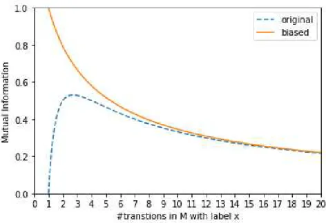
An important remark about this formulation to compute our measure inspired in mutual information is that it is not monotonous and it is equal to 0 if all the transitions of the specification are pairwise different. Since we are interested in values that are useful to compare test suites (therefore, we need monotony and we should avoid to “divide by zero”), we can solve this problem with a simple transformation. The dashed curve in Figure 3.2 shows the behaviour of the previous formula. We will do a small translation in the X axis of the logarithm of the formula, so that its behaviour is the one given by the solid curve. Definition 9. Let M be an FSM and t₁, t₂ be tests for M. Let ξ_t

1, ξt2 be the pseudo-random variables corresponding, respectively, to t1 and t2 and according to M. We have that the

modified mutual information formula will be

BMI(ξt1;ξt2) = X y∈t2 y∈mM X x∈t1 x=y log2(m+ 1) m

Figure 3.2: Measure comparison plot.

We will call this formula biased mutual information (BMI).

In the following example we illustrate the importance of this translation.

Example 2. Consider the FSM _{M depicted in Figure 3.3 and the test suites T1 = {t1 =} (i2i1i1, o2o1o1), t2 = (i2i4i4, o2o4o4)} and T2 = {t3 = (i3i1i1, o3o1o1), t4 = (i3i2i2, o3o2o2)}.

Note that the only pair appearing in botht1 andt2 is(i2, o2)(this transitions appears9times

in M); similarly, the only common pair for t3 and t4 is (i3, o3) (this transitions appears 1

time in M). The (biased) mutual information of each test suite can be computed as follows:

BMI(ξt1;ξt2) = log2(9 + 1) 9 = log2(10) 9 ≈0.3691 BMI(ξt3;ξt4) = log2(1 + 1) 1 = log2(2) 1 = 1 I(ξt1;ξt2) = log2(9) 9 ≈0.3522 I(ξt3;ξt4) = log2(1) 1 = 0

Therefore, the first test suite would be better if we consider biased mutual information, but would be worse if we consider mutual information. In principle, we should preferT because

q16 q15 q14 q0 q1 q2 q3 q19 q18 q17 q5 q6 q7 q8 q21 q20 q22 q11 q12 q4 q10 q23 q9 q13 i1/o1 i2/o2 i3/o3 i1/o1 i1/o1 i2/o2 i 2/o2 i2/o2 i1/o1 i1/o1 i1/o1 i2/o2 i2/o2 i1/o1 i2/o2 i1/o1 i1/o1 i2/o2 i2/o2 i2/o2 i1/o1 i4/o4 i4/o4 Figure 3.3: Example of FSM.

it is more likely that it will check more transitions thanT2. In fact, in this example we know

that the second test suite will traverse the same transition twice.

We are aware that the previous example shows that BMI works in one (ad hoc) example. In the next section, we will present experimental evidence to show that this measure works for randomly generated systems.

So far, we have defined biased mutual information for a test suite consisting of two tests. Fortunately, it is very easy to extend our notion to deal with more than 2 tests. This is so because we do not need to know the biased mutual information between all the sequences of (input/output) pairs of the test suite; we need to compute the cumulative amount of biased mutual information between all the possible pairs of these sequences (so it is easily done with a summation). Therefore, if we have a specification M (as usually, we omit M in the following notation) and a test suite T ={t1, . . . , tk} then

I(T) =I(ξt1, . . . , ξtk) = X i=1_,...,k X j=_i+1_,...,k I(ξti, ξtj) =

=X i=1,...,k X j=i+1,...,k X y∈ti X x∈tj σξ_{tj ,ti}(x, y)·log2 σξ_{tj ,ti}(x, y) σξ_tj(x)·σξ_ti(y)

Now, using Lemma 1 and Definition 9, we have that the biased mutual information of T is

BMI(ξt1, . . . , ξtk) = X i=1,...,k X j=i+1,...,k X y∈_ti y∈mM X x∈_tj x=y log2(m+ 1) m

We have to add to the previous expression the biased mutual information of each test of the test suite. This is computed as:

BMI(ξt;ξt) = X y∈_nt y∈mM (n−1)·n 2 · log2(m+ 1) m

This addition allows us to give a more precise formulation because it will give lower priority to tests corresponding to the repeated traversal of a loop in the specification. In fact, we are penalising the repetition of the same (input/output) pair (and therefore, potentially the same transition) in the test.

Therefore, the final formula to compute the biased mutual information of a test suite T

is given in the following definition.

Definition 10. Let M be an FSM_{andT ={t1, . . . , tk} be a test suite for M. Letξt}

1, . . . , ξtk

be the pseudo-random variables corresponding, respectively, tot1, . . . , tkand according to M.

We have BMI(ξt1, . . . , ξt_k) = X i=1,...,k X y∈_nti y∈mM    X j=i+1,...,k X x∈_tj x=y log2(m+ 1) m + (n−1)·n 2 · log2(m+ 1) m   

In the next chapter of this thesis we will describe several experiments confirming that our measure works reasonably good to choose among two different test suites the one that has more potential to detect faults in the SUT.

Chapter 4

Empirical evaluation

In this chapter we show our results concerning the usefulness of our measure to choose good

test suites. First, we clearly state our research questions.

4.1

Research questions

In order to test our measure, we will first check how wellit works.

Research Question 1. Are lower levels of biased mutual information associated with higher fault coverage?

If we have a positive answer (with statistical relevance) to this question, then we would like to see how our strategy compares to a purely random choice and with currently proposed Information Theory measures.

Research Question 2. Have test suites selected by biased mutual information higher fault coverage than the ones randomly selected?

Research Question 3. Have test suites selected by biased mutual information higher fault coverage than the ones selected by test set diameter (TSDm)?

Finally, we would like to check whether our measure is time consuming in a way such that it might be better to use the time needed to compute the measure to apply additional tests.

Research Question 4. How does the time to execute the selection method scale as the size of the test suite increases? How does the time needed to compute the selection method relate to the time needed to apply a test suite?

Before we show the results of the experiments, we briefly describe how our FSM subjects

are computed.

4.2

FSM Generator

In order to perform our experiments we need to generate FSMs. We developed an FSM

generator that randomly generates FSMs given some parameters. We used the OpenFST

library [1]1_{to represent}

FSMs. Once we had a proper representation of ourFSMs, we developed

a tool to generate these FSMs. In order to have a general tool that can be used in a range of

experiments, we included some basic parameters:

• NREP: the number of FSMs that we want to generate.

• MAX_ST AT ES: the maximum number of states an FSM can have.

• MIN_ST AT ES: the minimum number of states an FSMmust have.

• MAX_T RANSIT IONS: the maximum number of transitions each state of anFSM

can have.

• MIN_T RANSIT IONS: the minimum number of transitions each state of an FSM

must have.

• NUM_INP UT S: the number of inputs.

• NUM_OUT P UT S: the number of outputs. 1

This library is intended to work with Finite State Transducers (as its name indicates). These are a kind of FSMs with an (input/output) pair in each transition and a weight. Therefore, we simply ignored the weight.

Result: NREP FSMs. machine= 0;

while machine < NREP do

Set a random number S of states between MIN_ST AT ES and

MAX_ST AT ES for the FSM;

Choose the state 0as initial state;

for each state 0≤i < S −1 of the machine do

Set a random number T of transitions between MIN_T RANSIT IONS

and MAX_T RANSIT IONS for the state; for each transition 0≤j < T of the state do

if j == 0 then

Set the state i+ 1 as the end of the transition; else

Set a random state as the end of the transition; end

Set a random input label for the transition; Set a random output label for the transition; Save this transition to the FSMfile;

end end

Create the binary file that the OpenFST library uses;

machine+ +; end

Algorithm 2: FSM generation algorithm.

After setting these basic parameters, the program can be executed. The execution flow for generating an FSM using our tool is given in Algorithm 2. Note that, by construction,

the tool returns connected FSMs (all states are reachable from the initial state).

In order to create input-enabled FSMs with our tool we simply set:

MIN_T RANSIT IONS =MAX_T RANSIT IONS =NUM_INP UT S

4.3

Experiments

In order to answer our research questions, we performed different experiments. The first ones tries to address RQ1, RQ2 and RQ4, while the last ones tries to answer RQ3. The code developed to answer these questions has an MIT license and can be downloaded from

Figure 4.1: Schema of our experiment scenario.

4.3.1

Measure convenience

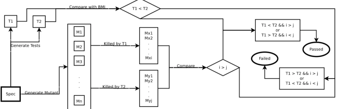
First, we need to know if our measure is valid for our purposes. In order to do so we will follow the schema presented in Figure 4.1. We started with 100 randomly generated FSMs.

These FSMs had 50 states. Each state has a random number, between 2 and 5, of outgoing transitions. Each transition will have a pair (input/output) where the input and output alphabets have 5 elements 2_.

For each FSM, we first go through it storing all the possible (input/output) labels of the

transitions and the number of times a label appears. Then, we generate 2 test suites, of size 100, from theFSMrepresenting the specification3 _{and compute our measure to chose the} best one. Finally, we produce 1000 mutants of the original FSM. We only use the mutation

operator consisting in modifying the incoming state of a transition because our experiments showed that mutations on the labels of the transitions are easier to detect during testing.

We apply the test suites to the mutants and compute which test suite kills more mutants. We repeat this procedure for each FSMand then compute how many times our selected test

suite was the one that killed more mutants. We produce apercentage of success, that is, how many times the test suite chosen by our measure was the one killing more mutants (in case

2

Later, we will see experiments with alphabets of different size, FSMs with different number of states and/or different number of outgoing transitions. We do not report results on these scenarios because they are similar to the ones presented in this thesis.

3

of ties, either concerning the value of our measure or the number of killed mutants, we avoid this result). We repeated the whole process 50 times, getting 50 different percentages of success (each percentage is obtained from100differentFSMs). Therefore, the final percentage

is computed after repeating the experiment 5000 times.

The results of our experiments are given in Table4.1. First, we randomly generated test suites without any checking. Therefore, our initial test suites had repeated and/or redundant tests 4_{. In this setting, the results show that our measure is very good: the percentage of}

success was 62.2402%. Then, we ensured that our test suites did not have either repeated tests or prefixes of another test. Our results where almost the same: we got, on average, a percentage of success equal to 62.4924%. Therefore, our measure is equally good given any kind of test suite and, very important, none of the experiments showed a result with a percentage of success lower than 50%. An important remark we have to do is that this scenario is a very complex one, due to the small alphabet. The complexity comes from the fact that with FSMs with smaller alphabets, it is easier that in a test a (input/output) pair

is repeated. This leads to bigger similarity in the test suites and therefore it is harder to detect differences. In the next section we will discuss what happens when we have bigger alphabets.

In Table 4.2 we display a summary of these results, where we can see that they are almost the same. We have only a small difference between the percentages of success. We think that it was be produced due to the randomness associated with the process. Also, we can see that in both cases, all the values are in the range [0.5−0,8), with the majority of them belonging to the range [0.6−0.7). Finally, we can see that there are almost no differences between the maximum and minimum values. These observations reinforce the idea that our measure is equally good if we allow the test suite to have repeated tests or not. Therefore, and thinking as we would do when doing proper testing, during the rest of the experiments we will always consider the case where we do not allow the test suite to

4

Note that in this specific situation, a test suite will be a multi-set of tests instead of a set. This is so because we need to take into account how many times a certain test appears in the test suite.

Run Number With possible without

repetition of tests repetition of tests

1 0.65 0.555556 2 0.59596 0.62 3 0.666667 0.535354 4 0.602041 0.62 5 0.71 0.642857 6 0.58 0.59596 7 0.66 0.612245 8 0.56 0.65 9 0.65 0.585859 10 0.656566 0.71 11 0.69697 0.520408 12 0.59 0.646465 13 0.63 0.656566 14 0.63 0.636364 15 0.602041 0.737374 16 0.58 0.71 17 0.663265 0.636364 18 0.606061 0.646465 19 0.616162 0.581633 20 0.65 0.608247 21 0.585859 0.686869 22 0.59 0.57 23 0.540816 0.666667 24 0.653061 0.61 25 0.565657 0.626263 26 0.602041 0.61 27 0.61 0.587629 28 0.670103 0.63 29 0.639175 0.618557 30 0.632653 0.636364 31 0.540816 0.59596 32 0.626263 0.57 33 0.618557 0.632653 34 0.68 0.585859 35 0.6 0.646465 36 0.606061 0.64 37 0.58 0.57 38 0.66 0.61 39 0.59 0.626263 40 0.69697 0.663265 41 0.656566 0.69697 42 0.545455 0.656566 43 0.59 0.63 44 0.714286 0.656566 45 0.6 0.540816 46 0.571429 0.642857 47 0.63 0.61 48 0.606061 0.61 49 0.61 0.628866 50 0.714286 0.68

Type of #runs #runs #runs min value max value %success test suite [0.5,0,6) [0.6,0.7) [0.7,0.8) (mean)

with possible repetitions 15 32 3 0.540816 0.714286 62.2402%

without repetitions 13 34 3 0.520408 0.737374 62.4924%

Table 4.2: Summary of the results of the first experiment. have neither repeated nor redundant tests.

4.3.2

Measure analysis

Once we can claim, with experimental evidence, that our measure works, we would like to do a sanity check. We repeated the experiments using the same FSMs but different

test suites and mutants, and evaluated what is the correlation between our measure score and the mutation score (i.e. the number of killed mutants). We obtained an average Pearson correlation of −0.369134 and an average Spearman correlation of −0.356978. The fact that the correlations are negative implies that lower scores of our measure will obtain higher mutation scores, what gives us an affirmative answer to RQ1. More important, these correlations are consistent with the results from the previous experiment. Specifically, if we select the test suite with lower biased mutual information, then we will be selecting the test suite that kills more mutants approximately 62% of the times. This implies that the correlation should be negative. The full results are displayed in Table 4.3.

In order to decide how well our measure performs in terms of time, we realized another experiment. For this experiment, we produced 100 new FSMs, with the same parameters as

before, but with a bigger alphabet (specifically, of size 25). We wanted to check how the results can change in a more relaxed scenario. We generated test suites without repetitions because the previous experiments show that the results are nearly the same. This time we also recorded the time that it takes to compute our measure (we will use these values to assess the performance of our measure). The results are given in Table 4.4.

On average, the percentage of success was75.0605%. These results are much better than the results from the first experiments. So we can conclude that our method works better in

Run Number Pearson correlation Spearman correlation 1 −0.378529 −0.447121 2 −0.407239 −0.308503 3 −0.305347 −0.299361 4 −0.338248 −0.257336 5 −0.342747 −0.374436 6 −0.634282 −0.541008 7 −0.731647 −0.731102 8 −0.273694 −0.312782 9 −0.247209 −0.220384 10 −0.395459 −0.409929 11 −0.259926 −0.298081 12 −0.170457 −0.0308619 13 −0.414295 −0.456907 14 −0.507343 −0.693233 15 −0.58775 −0.624765 16 −0.44744 −0.545865 17 0.123024 0.232103 18 −0.383787 −0.300752 19 −0.534142 −0.471783 20 0.00977185 −0.0647103 21 −0.505013 −0.486649 22 −0.354695 −0.484575 23 −0.492013 −0.408578 24 −0.357769 −0.355907 25 −0.460478 −0.391877 26 −0.584937 −0.660399 27 −0.425394 −0.415194 28 −0.224411 −0.227905 29 −0.495339 −0.596992 30 −0.674246 −0.603391 31 −0.0656146 0.00300865 32 −0.468773 −0.438511 33 −0.433851 −0.395637 34 −0.564793 −0.456735 35 −0.553955 −0.548872 36 −0.383386 −0.40271 37 −0.285205 −0.221302 38 0.110759 0.0721805 39 −0.689946 −0.61203 40 −0.664481 −0.54778 41 −0.333295 −0.275188 42 −0.328676 −0.34501 43 −0.158634 −0.202484 44 −0.0459975 0.0428894 45 −0.245797 −0.300113 46 −0.380434 −0.359398 47 −0.325745 −0.26968 48 −0.462855 −0.37594 49 −0.132061 −0.17833 50 −0.242898 −0.248966

Run Number Percentage of success Elapsed Time 1 0.76 0.000842141 2 0.721649 0.000793936 3 0.85 0.000822785 4 0.767677 0.000821019 5 0.826531 0.000813211 6 0.680412 0.000838903 7 0.77 0.000841091 8 0.74 0.000789195 9 0.806122 0.000826917 10 0.707071 0.000835529 11 0.717172 0.000853626 12 0.74 0.00082674 13 0.8 0.000840832 14 0.787879 0.000840821 15 0.76 0.00086412 16 0.75 0.000841077 17 0.714286 0.000850253 18 0.69 0.00082661 19 0.747475 0.0008403 20 0.714286 0.000846815 21 0.707071 0.000871455 22 0.65 0.000806566 23 0.757576 0.000827078 24 0.7 0.000842363 25 0.77 0.000819572 26 0.76 0.000836346 27 0.693878 0.00083186 28 0.717172 0.00085203 29 0.74 0.000836536 30 0.76 0.00085497 31 0.767677 0.000844704 32 0.795918 0.000847846 33 0.767677 0.000852514 34 0.78 0.000832202 35 0.71 0.000828946 36 0.795918 0.000863082 37 0.767677 0.000832604 38 0.83 0.000833852 39 0.83 0.000831776 40 0.838384 0.000874901 41 0.636364 0.000850119 42 0.737374 0.000826633 43 0.83 0.000844154 44 0.767677 0.000823715 45 0.686869 0.000835953 46 0.747475 0.000843442 47 0.69 0.000844199 48 0.73 0.000821044 49 0.7 0.000852965 50 0.814433 0.000873662

FSMs with big alphabets.

Concerning time, on average we needed 0.00083786 seconds for the computation of our measure for test suites of size 100.5 _{Therefore, we needed a time of the order of thousandths}

of a second to compute our measure for all the test suites used in our experiment. In principle, we can conclude that the time needed to compute our measure is acceptable for our purposes but we would like to compare this time with the time needed to apply a test suite, so we performed another experiment.

As a performance check, in order to answer RQ4 we repeated the previous experiment as follows. First, we recorded the time needed to compute our measure for test suites of size

100, 200, 300, 400, 500, 600, 700, 800, 900 and 1000. We also recorded the time needed to apply these test suites over 1000 mutants assuming that the time needed to execute a transition is 0, 0.000001, 0.00001, 0.0001, 0.001, 0.01, 0.1 and 1 seconds. Note that in our setting, the execution of a transition is instantaneous but if we test a real system, then there will be a delay, depending on the computations needed to compute the result, between the application of an input and the reception of an output. Also note that we do not need to assume these delays when computing our measure because we compute it using only the specification and the involved test suites: neither test application nor transition executions are needed. With all these values, we compared the average time needed to compute our measure over one test suite versus the average time needed to apply a test suite over a mutant and we got the results that we can see in Figure 4.2. It is important to note that the average time to compute our measure includes the time needed to generate the map of I/O pairs from the specification. This time depends on the size of the specification and it is computed only once for all the measure computations. Therefore, although we added it to the time needed to compute our measure for one test suite, computing it for two test suites will not double the time. Instead, it will simply add the time that is reflected on the plot

5

The experiments were run on a GNU/Linux machine with an AMDR Ryzen threadripper 1920X at

3.50GHz×12 cores and with 32GB of RAM (although only one core was running at a time and we did not

for transition time equal to 0 because, in this case, the time needed to generate the I/O pairs map is assumed to be 0.

As we can deduce from Figure 4.2, as long as the time needed to perform a transition is higher than 0.001seconds, computing our measure is much faster than applying test suites. If this time is higher than0.1seconds then we need minutes (or even hours if it is higher than

1second) to apply a test suite. As an additional result of our experiments, we validated that the time needed to compute our measure scales (approximately) quadratically with respect to the test suite size.

This last fact is important because the time to execute a test suite follows a nearly logarithmic scale with respect to the test suite size. This is so because we are cutting the execution of a test whenever we found a failure, as this implies that the implementation does not pass the test. Note that if we would continue the execution after a failure is found, then the scale in time should be (nearly) lineal. Anyway, there will always be a test suite size where the time needed to select a test suite will be equally to the time needed to execute a test suite. Therefore, we should take into account that for some test suites it will be better to execute two test suites than to select one using our measure.

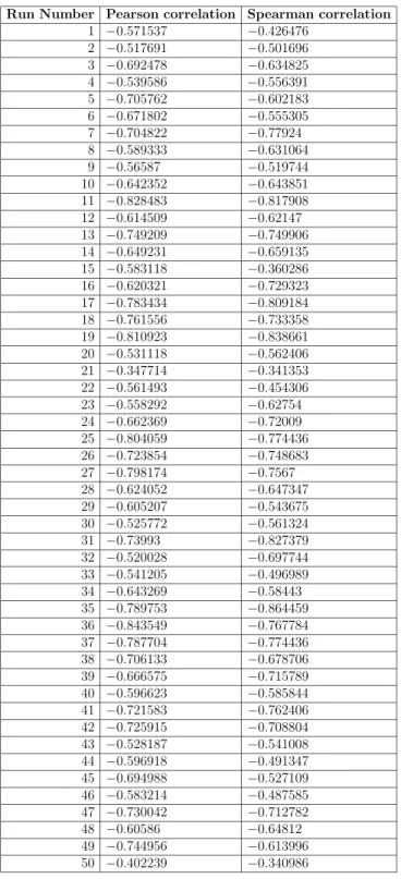
Finally, in order to observe the consistency in the Pearson and Spearman correlations between our measure and mutation scores, we repeated the experiment that started this section. However, this time we used the FSMs having an alphabet of 25 elements that we used in the last two experiments. The results show that the consistency holds because we got even better correlations. Specifically, we obtained an average Pearson correlation of

−0.650256and an average Spearman correlation of−0.634711. The full results are displayed on Table 4.5.

4.3.3

Measure comparison

Finally, we wanted to compare our measure with previous proposals. In this regard, we compared our measure with the Test Set Diameter (TSDm) measure and method [16].

Figure 4.2: Time comparison plots (from left to right, from top to bottom, with transition time of 0, 0.000001, 0.00001, 0.0001, 0.001, 0.01, 0.1and 1seconds).

Run Number Pearson correlation Spearman correlation 1 −0.571537 −0.426476 2 −0.517691 −0.501696 3 −0.692478 −0.634825 4 −0.539586 −0.556391 5 −0.705762 −0.602183 6 −0.671802 −0.555305 7 −0.704822 −0.77924 8 −0.589333 −0.631064 9 −0.56587 −0.519744 10 −0.642352 −0.643851 11 −0.828483 −0.817908 12 −0.614509 −0.62147 13 −0.749209 −0.749906 14 −0.649231 −0.659135 15 −0.583118 −0.360286 16 −0.620321 −0.729323 17 −0.783434 −0.809184 18 −0.761556 −0.733358 19 −0.810923 −0.838661 20 −0.531118 −0.562406 21 −0.347714 −0.341353 22 −0.561493 −0.454306 23 −0.558292 −0.62754 24 −0.662369 −0.72009 25 −0.804059 −0.774436 26 −0.723854 −0.748683 27 −0.798174 −0.7567 28 −0.624052 −0.647347 29 −0.605207 −0.543675 30 −0.525772 −0.561324 31 −0.73993 −0.827379 32 −0.520028 −0.697744 33 −0.541205 −0.496989 34 −0.643269 −0.58443 35 −0.789753 −0.864459 36 −0.843549 −0.767784 37 −0.787704 −0.774436 38 −0.706133 −0.678706 39 −0.666575 −0.715789 40 −0.596623 −0.585844 41 −0.721583 −0.762406 42 −0.725915 −0.708804 43 −0.528187 −0.541008 44 −0.596918 −0.491347 45 −0.694988 −0.527109 46 −0.583214 −0.487585 47 −0.730042 −0.712782 48 −0.60586 −0.64812 49 −0.744956 −0.613996 50 −0.402239 −0.340986

TSDm method

The TSDm method [16] produces a test suite from a pool of tests. This method uses test set diameter (TSDm) measures as a guide to generate test suites. In order to assess the suitability of our measure, we will use it in combination with the TSDm method to evaluate its goodness with respect to different test set diameter measures.

Specifically, we select in each step, from a pool of tests, the test that will be removed from the test suite. In other words, if we take out this test from the pool, then the test suite conformed by the remaining tests of the pool has the best score6 _{of the measure when}

compared to the test suites that will be produced from taking out another test from the pool. This process is iteratively performed until we obtain a test suite of the desired size.

In order to perform the comparison, we started using the same 100 FSMs from the first

experiment. For each FSM, we first go through it storing all the possible (input/output)

labels of the transitions and the number of times a label appears. Then we produced two test suites of size100executing the TSDm method over the same pool of100tests, using the Input-TSDm (ITSDm) measure for one test suite and our BMI for the other test suite. After that, we produce 1000 mutants of the original FSM, with mutations consisting, as before, in

changing the target state of a transition to another state. The states of the mutants are completed with bogus self-loop transitions to ensure input-enabledness.

Finally, we computed the mutation score applying the test suites to the mutants. We repeated this procedure for each FSM and then computed how many times the test suite

generated using BMI was the one with higher mutation score. With this result we produced a percentage of success, that is, how many times the test suite generated with our measure was the one with higher mutation score (in case of ties on the number of killed mutants, as usual, we avoid this result). We repeated the whole process 50 times, getting 50 different percentages of success (each percentage is obtained from100 different FSMs). Therefore, the

final percentage is computed after repeating the experiment 5000 times. 6

Run Number Percentage of success BMI Percentage of success ITSDm 1 0.857143 0.142857 2 0.880952 0.119048 3 0.875 0.125 4 0.864865 0.135135 5 0.891892 0.108108 6 0.871795 0.128205 7 0.906977 0.0930233 8 0.809524 0.190476 9 0.904762 0.0952381 10 0.828571 0.171429 11 0.948718 0.0512821 12 0.875 0.125 13 0.809524 0.190476 14 0.853659 0.146341 15 0.909091 0.0909091 16 0.863636 0.136364 17 0.847826 0.152174 18 0.886364 0.113636 19 0.933333 0.0666667 20 0.875 0.125 21 0.918919 0.0810811 22 0.888889 0.111111 23 0.833333 0.166667 24 0.833333 0.166667 25 0.844444 0.155556 26 0.897436 0.102564 27 0.9 0.1 28 0.854167 0.145833 29 0.926829 0.0731707 30 0.930233 0.0697674 31 0.893617 0.106383 32 0.893617 0.106383 33 0.911111 0.0888889 34 0.945946 0.0540541 35 0.906977 0.0930233 36 0.883721 0.116279 37 0.883721 0.116279 38 0.897436 0.102564 39 0.866667 0.133333 40 0.909091 0.0909091 41 0.92 0.08 42 0.837209 0.162791 43 0.894737 0.105263 44 0.904762 0.0952381 45 0.956522 0.0434783 46 0.857143 0.142857 47 0.930233 0.0697674 48 0.854167 0.145833 49 0.869565 0.130435 50 0.948718 0.0512821

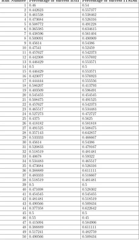
The results of the experiment took a lot of time to compute. So, we only managed to obtain the first result and the percentage of success was 100%. However, we realized that our measure took around78% more time to produce the better test suite than the ITSDm. This could be considered as a kind of cheating: our measure is much better but it takes much longer to compute it. Therefore, we decided to perform two quicker experiments.

The first one consists in cutting the times to the half. In order to do so, as we cannot cut off the computation of the measure, we decided to reduce the pool for the BMI measure to a 50%of the pool that the ITSDm will have to produce the test suite. Then, the pool for BMI corresponds to the first50tests from the pool of the ITSDm, although our experiments show that it would be essentially the same to select any50tests from the ITSDm pool. The results of this experiment are given in Table 4.6. They show that our measure is very good: the percentage of success was 88.5836%, what implies that with half of the resources, our measure clearly outperforms ITSDm.

The last experiment comes from the decision to give both measures the same time to produce the test suite. In order to do so, we shrink the pool for BMI to 22 tests from the pool of the ITSDm. The results of the experiment are given in Table 4.7. As we can see, a curious effect appears: our measure is better only 46.89% of the time. So, we have slightly worse results but we have a handicap of 78%. More important, there are runs where our measure gets a success score of more than 50%.

TSDm measure

We wanted also to test our measure versus the TSDm measure in a more active way. Instead of choosing from a pool of randomly generated test suites, we wanted to compare how good is each measure in order to create a good test suite. Then, we wanted to compare their performance as a measure to guide an evolutive programming method to generate test suites.

In order to do so, we will use the tool that we developed during this academic year. The tool is able to generate test suites using Genetic Programming [25]. The framework and

Run Number Percentage of success BMI Percentage of success ITSDm 1 0.46 0.54 2 0.442623 0.557377 3 0.461538 0.538462 4 0.473684 0.526316 5 0.508772 0.491228 6 0.365385 0.634615 7 0.438596 0.561404 8 0.509091 0.490909 9 0.45614 0.54386 10 0.47541 0.52459 11 0.457627 0.542373 12 0.442308 0.557692 13 0.446429 0.553571 14 0.5 0.5 15 0.446429 0.553571 16 0.423077 0.576923 17 0.444444 0.555556 18 0.586207 0.413793 19 0.403509 0.596491 20 0.545455 0.454545 21 0.508475 0.491525 22 0.457627 0.542373 23 0.465517 0.534483 24 0.527273 0.472727 25 0.4375 0.5625 26 0.418182 0.581818 27 0.491525 0.508475 28 0.357143 0.642857 29 0.533333 0.466667 30 0.45614 0.54386 31 0.520833 0.479167 32 0.518519 0.481481 33 0.40678 0.59322 34 0.534483 0.465517 35 0.473684 0.526316 36 0.388889 0.611111 37 0.483333 0.516667 38 0.518519 0.481481 39 0.5 0.5 40 0.471698 0.528302 41 0.454545 0.545455 42 0.481481 0.518519 43 0.490566 0.509434 44 0.377358 0.622642 45 0.5 0.5 46 0.55 0.45 47 0.415094 0.584906 48 0.388889 0.611111 49 0.517241 0.482759 50 0.490566 0.509434

implementation of the tool are explained later on Section 4.5; here we will only discuss the results of this comparison.

We decided to make an extensive comparison of our measure versus the possible versions of the TSDm measure. Specifically, we decided to compare BMI with the Input-TSDm (ITSDm), the Output-TSDm (OTSDm) and the InputOutput-TSDm (IOTSDm). This way, we cover all the possibilities that we have to use the TSDm measure when working in a black-box scenario. Also, in order to address some of the threats to the validity of our results that we will discuss later, we changed the FSMs that the tool provides to make the

comparison by the 100 FSMs that we have been using in our experiments.

The results can be seen in Tables 4.8 (ITSDm), 4.9 (OTSDm) and 4.10 (IOTSDm). As we can see, our measure got better results in all the three comparisons. For ITSDm, BMI killed more mutants 70.5488%of the times, killing an average of 48.5651% of the mutants, while ITSDm killed more mutants 29.4512% of the times, killing an average of 45.5551%

of the mutants. Similarly, for OTSDm, BMI killed more mutants 71.0744% of the times, killing an average of49.2625%of the mutants, while OTSDm killed more mutants28.9256%

of the times, killing an average of 45.1924% of the mutants. Finally, for IOTSDm, BMI killed more mutants 66.9494%of the times, killing an average of 48.8414% of the mutants, while IOTSDm killed more mutants 33.0506%of the times, killing an average of 46.5447%

of the mutants.

With these results, we can conclude that the measure that gets a better performance against BMI is IOTSDm. In any case, none of them managed to get better results than our measure in the majority of the runs. Therefore, we can claim that our measure is better, in order to generate tests suites, than the test set diameter measures.

4.4

Research questions answers

As a recap of all the results that we obtained along all the experiments, we can answer the Research Questions we performed at the beginning of this chapter.

Run Percentage of Percentage of Percentage of killed Percentage of killed Number success BMI success ITSDm mutants by BMI mutants by ITSDm

1 0.72619 0.27381 0.501798 0.446298 2 0.666667 0.333333 0.466654 0.479782 3 0.730769 0.269231 0.493308 0.418359 4 0.725 0.275 0.512737 0.462038 5 0.666667 0.333333 0.425722 0.459042 6 0.682353 0.317647 0.468518 0.498447 7 0.692308 0.307692 0.466859 0.454359 8 0.702703 0.297297 0.452919 0.431595 9 0.733333 0.266667 0.498853 0.42044 10 0.830986 0.169014 0.509408 0.368718 11 0.653846 0.346154 0.464744 0.481641 12 0.75 0.25 0.453184 0.436276 13 0.613333 0.386667 0.48644 0.520147 14 0.703704 0.296296 0.500951 0.459642 15 0.696203 0.303797 0.518215 0.463215 16 0.707317 0.292683 0.515537 0.459268 17 0.75641 0.24359 0.475551 0.440897 18 0.670886 0.329114 0.509975 0.478494 19 0.728571 0.271429 0.477114 0.426729 20 0.7 0.3 0.513737 0.475263 21 0.701299 0.298701 0.525195 0.437857 22 0.736842 0.263158 0.458303 0.414711 23 0.666667 0.333333 0.485393 0.477429 24 0.7 0.3 0.525543 0.476471 25 0.691358 0.308642 0.412543 0.472506 26 0.68 0.32 0.47492 0.440453 27 0.736111 0.263889 0.437694 0.44525 28 0.697368 0.302632 0.513342 0.466895 29 0.746667 0.253333 0.507933 0.440147 30 0.666667 0.333333 0.490747 0.432093 31 0.6375 0.3625 0.425737 0.48605 32 0.675676 0.324324 0.488392 0.473122 33 0.679487 0.320513 0.517949 0.469654 34 0.642857 0.357143 0.496655 0.521512 35 0.773333 0.226667 0.513773 0.422067 36 0.75 0.25 0.560369 0.419286 37 0.662338 0.337662 0.496286 0.493156 38 0.842105 0.157895 0.52675 0.373513 39 0.763158 0.236842 0.455658 0.415053 40 0.696203 0.303797 0.519494 0.454 41 0.682927 0.317073 0.490073 0.503963 42 0.618421 0.381579 0.425632 0.477 43 0.769231 0.230769 0.457026 0.405397 44 0.707317 0.292683 0.518951 0.436354 45 0.684932 0.315068 0.397822 0.486041 46 0.782051 0.217949 0.510462 0.407321 47 0.675 0.325 0.443737 0.498713 48 0.728395 0.271605 0.484185 0.45637 49 0.692308 0.307692 0.502397 0.483474 50 0.671053 0.328947 0.490763 0.485961

Run Percentage of Percentage of Percentage of killed Percentage of killed Number success BMI success OTSDm mutants by BMI mutants by OTSDm

1 0.671053 0.328947 0.469737 0.469513 2 0.716049 0.283951 0.443963 0.444654 3 0.706667 0.293333 0.509373 0.433827 4 0.6625 0.3375 0.51235 0.470938 5 0.772152 0.227848 0.492114 0.413241 6 0.7375 0.2625 0.4797 0.432113 7 0.82716 0.17284 0.514617 0.376037 8 0.662162 0.337838 0.497973 0.474189 9 0.65 0.35 0.455862 0.497288 10 0.72 0.28 0.424533 0.427547 11 0.768293 0.231707 0.500756 0.433927 12 0.674699 0.325301 0.516904 0.496217 13 0.688312 0.311688 0.478065 0.439857 14 0.716216 0.283784 0.507824 0.455189 15 0.743902 0.256098 0.509695 0.420878 16 0.74026 0.25974 0.467909 0.428377 17 0.73494 0.26506 0.500229 0.452181 18 0.697368 0.302632 0.479408 0.489118 19 0.693333 0.306667 0.49524 0.4992 20 0.717949 0.282051 0.429705 0.445808 21 0.631579 0.368421 0.414434 0.493724 22 0.675 0.325 0.511787 0.420313 23 0.675325 0.324675 0.504247 0.472584 24 0.783784 0.216216 0.589486 0.415959 25 0.6 0.4 0.4587 0.516563 26 0.649351 0.350649 0.459545 0.469156 27 0.739726 0.260274 0.515932 0.43737 28 0.703704 0.296296 0.496481 0.437605 29 0.691358 0.308642 0.477136 0.486815 30 0.717949 0.282051 0.466821 0.448103 31 0.684932 0.315068 0.47074 0.491438 32 0.72 0.28 0.547787 0.481773 33 0.712329 0.287671 0.493822 0.439699 34 0.74359 0.25641 0.554 0.423615 35 0.674419 0.325581 0.49086 0.461756 36 0.695122 0.304878 0.534622 0.466829 37 0.704225 0.295775 0.482155 0.462211 38 0.782051 0.217949 0.457526 0.398359 39 0.74359 0.25641 0.451513 0.433064 40 0.771429 0.228571 0.517071 0.401386 41 0.692308 0.307692 0.472885 0.468487 42 0.689189 0.310811 0.521703 0.475824 43 0.671053 0.328947 0.475263 0.488539 44 0.675 0.325 0.511925 0.458288 45 0.779221 0.220779 0.512506 0.425143 46 0.72973 0.27027 0.493946 0.460041 47 0.68 0.32 0.52008 0.442267 48 0.716216 0.283784 0.519041 0.453149 49 0.797297 0.202703 0.504824 0.411757 50 0.716049 0.283951 0.522815 0.452642