Cognitive Skills, Openness and Growth
Parantap Basu
yDurham University
Keshab Bhattarai
zUniversity of Hull
September 4, 2011
AbstractA signi…cant positive relationship exists between the ratios of trade and educational spending to GDP implying that countries which are more open on the trade front also spend more on education. An open economy en-dogenous growth model with human capital is developed to understand this stylized fact. The model predicts that countries with greater cognitive skills spend more on education, and grow faster. These countries open up on the trade front to …nance import of raw materials for investment goods produc-tion which becomes scarce due to the diversion of resources to educaproduc-tion. The model highlights the importance of the productivity of human capital or cognitive skill as an important economic fundamental determining the cross country correlation between growth, trade share and education share.
JEL Classi…cation: F41, O11, O33, O41
Keywords: Growth, Openness, Human capital, Cognitive Skill
Forthcoming in Economic Record. We have greatly bene…tted from useful comments made by two referees and the editor. The usual disclaimer applies.
yDepartment of Economics and Finance, Durham University, 23/26 Old Elvet,
Durham DH1 3HY, UK. e-mail: parantap.basu@durham.ac.uk.
zCorresponding Author, Business School, University of Hull, Hull, East
York-shire, HU6 7RX, UK. email:K.R.Bhattarai@hull.ac.uk.
This is the peer reviewed version of the following article: BASU, P. and BHATTARAI, K. (2012), Cognitive Skills, Openness and Growth. Economic Record, 88: 18–38, which has been published in final form at doi: 10.1111/j.1475-4932.2011.00764.x. This article may be used for non-commercial purposes in accordance With Wiley Terms and Conditions for self-archiving.
1
Introduction
While the relationships between trade openness and growth as well as growth and education have been well explored, little e¤ort has been made to under-stand these variables in an integrated growth model. Do open countries invest more in human capital? The issue is relevant for both empirical and theoret-ical reasons. It is well known that human capital is a vehicle of growth and growing economies are more open. A plethora of literature exists showing the connection between growth and education in a closed economy context (Barro (1991), Mankiw, Romer and Weil (1992), Jorgenson and Fraumeni
(1992), Parente and Prescott, (2002)).1 There is also a signi…cant volume
of literature addressing the issue of openness and growth (Grossman and
Helpman (1990), Manning (1982), Cartiglia (1997)).2 However, it is not
clear from the extant literature what common fundamentals link education, openness and growth. This paper is a quest for such fundamentals.
We propose that the cognitive skills of a country’s population are pow-erfully connected to growth, openness and education. The cognitive skills of pupils re‡ect the quality of schooling. Hanushek and Woessmann (2008) measure these cognitive skills by the Programme for International Student Assessment (PISA) test scores in mathematics and science, primary through the end of secondary school for all years (PISA scale divided by 100). They argue that di¤erences in quality of schooling make cognitive skills di¤er even though the years of schooling are the same across countries. This results in cross-country di¤erences in returns to schooling and growth rates.
1Bils and Klenow (2000), however, point out that the growth e¤ects of schooling may
be overestimated due to reverse causality from growth to schooling. Basu and Bhattarai (2011) show that the growth e¤ect of schooling could depend on the government bias in education.
2 Basu and Guariglia (2007) point out that FDI can complement human capital and
could be bene…cial for growth at the expense of greater inequality. Galor and Mountford (2008) further show that gains from trade are more directed towards investment in educa-tion and growth in OECD countries while these gains are more channelled towards higher fertility and population growth in case of developing countries.
The development facts that we present in the next section show that there is a signi…cant cross country positive correlation between trade share, educa-tion share and cognitive skills. This motivates us to develop an open economy growth model to understand this linkage. In our model, the principal driver of this skill-based technical change is cognitive skill. Higher cognitive skills of pupils could enhance the returns from schooling which provides the nation an incentive to divert raw labour from the goods to education sector. This gives rise to a relative scarcity of physical capital with respect to human capital. If the bulk of physical capital is made from imported raw materials from abroad, such a shortage makes it necessary for the economy to open up more on the trade front. Thus countries with higher cognitive skills invest more in education and also become more open on the trade front. We demon-strate this hypothesis in terms of an open economy endogenous growth model with human capital in the tradition of Becker (1975) and Lucas (1988). The paper derives closed form solutions for balanced growth rate, educational investment rate and openness showing how cognitive skills jointly determine all these three macroeconomic variables. To the best of our knowledge, our paper is the …rst in the literature which explores the role of cognitive skills in determining openness, education and growth within an endogenous growth model.
The rest of the paper is organized as follows. The following section doc-uments some development facts. Section 3 lays out the endogenous growth model. Section 4 describes the long run properties of the model. Section 5 performs short run analysis in terms of impulse responses. Section 6 con-cludes.
2
Some Development Facts
To gain empirical motivation, in this section we present some cross-country development facts about education, openness, growth and cognitive skills.
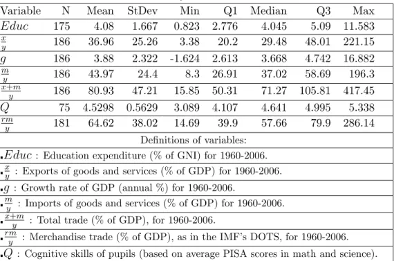
Table 1 reports the summary statistics for these variables. Data show enor-mous variations across countries. Among 186 countries, openness measured
by the ratios of exports xy , imports my and sum of exports and imports
(x+ym) to GDP vary remarkably. Small and highly developed countries like Singapore export around 221 percent of GDP followed by Aruba, Hong Kong, Luxemburg and Macao which have openness of more than 100 percent. On the other extreme, there are countries such as Argentina, Brazil, USA and India with exports less than 10 percent of their GDP. Only 45 countries in the world export more than 50 percent of their GDP. The median export ratio is 29 percent. Similar variation is seen in the education spending
ra-tio (Educ) among 175 countries. Countries like Guam, American Samoa
and New Caledonia spend more than 10 percent of gross national income (GNI) in education while countries like Laos, Congo, Chad, Haiti, Myanmar, Bangladesh, Somalia and Indonesia have less than 1.5 percent of their GNI in it. The range of cognitive skills in the sample of 77 countries is from 3.089 (South Africa) to 5.338 (South Korea). Average growth rate of GDP was 3.88 percent per year. Ukraine (-1.6 percent) and Bosnia and Herzegovina (16.9 percent) are outliers mainly because of missing data series.
To motivate our theoretical model where the home country produces in-vestment goods with the aid of imported raw materials, we take merchandise imports (de…ned in the IMF’s DOTS from the World Bank’s WDI database)
to be a good indicator of imported raw materials (rm). Such imports
in-clude spare parts, food, agricultural raw materials, fuels, ores & metals and
manufactured products. These imported raw materials are the US dollar
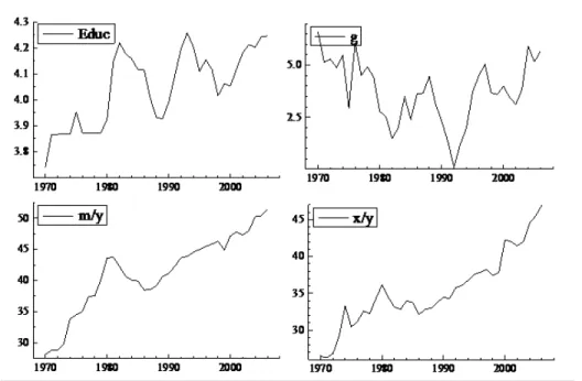
c.i.f value of goods purchased from the rest of the world as shown in Table 1. The trends of cross country averages of ratio of education spending to GNI, growth rates of GDP and ratios of imports and exports to GDP are shown in Figure 1 for the last thirty …ve years.3 The secular rising trends in
3See the note of Table 1 for de…nitions of variables and the Appendix B for the list of
Table 1: Summary Statistics: 1971-2007
Variable N Mean StDev Min Q1 Median Q3 Max
Educ 175 4.08 1.667 0.823 2.776 4.045 5.09 11.583 x y 186 36.96 25.26 3.38 20.2 29.48 48.01 221.15 g 186 3.88 2.322 -1.624 2.613 3.668 4.742 16.882 m y 186 43.97 24.4 8.3 26.91 37.02 58.69 196.3 x+m y 186 80.93 47.21 15.85 50.31 71.27 105.81 417.45 Q 75 4.5298 0.5629 3.089 4.107 4.641 4.995 5.338 rm y 181 64.62 38.02 14.69 39.9 57.66 79.9 286.14 De…nitions of variables: Educ: Education expenditure (% of GNI) for 1960-2006.
x
y : Exports of goods and services (% of GDP) for 1960-2006.
g : Growth rate of GDP (annual %) for 1960-2006.
m
y : Imports of goods and services (% of GDP) for 1960-2006. x+m
y : Total trade (% of GDP), for 1960-2006. rm
y : Merchandise trade (% of GDP), as in the IMF’s DOTS, for 1960-2006.
Q: Cognitive skills of pupils (based on average PISA scores in math and science).
import and export ratios indicate the rapid pace of globalization in the last four decades. This rise is associated with an increase in the ratio of education spending to GDP during this period.
2.1
Cross-country relationship between education,
open-ness and growth
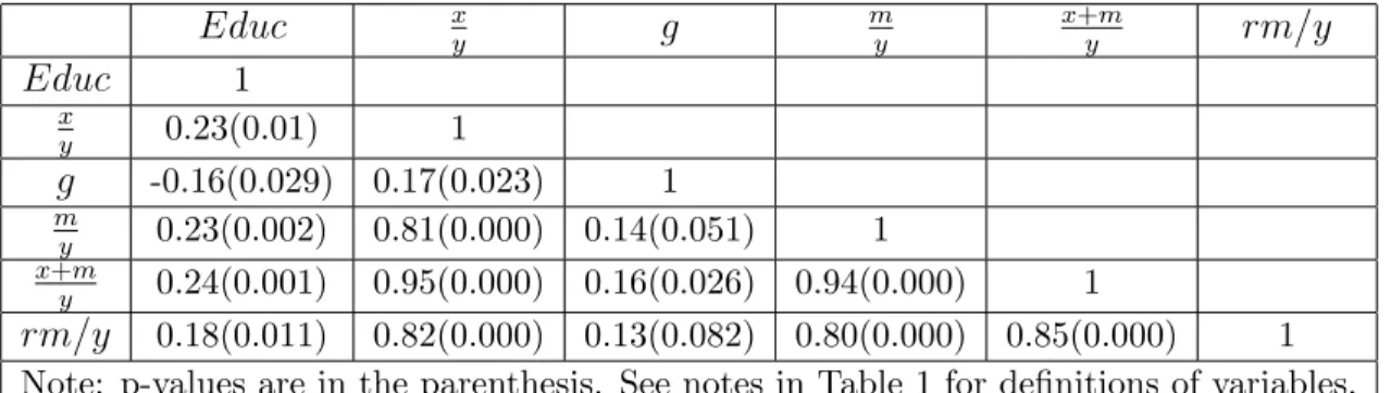
Table 2 reports the cross-country correlations between time averages of open-ness, growth and education spending ratios. Four measures of openness are
used, namely x=y; m=y,(x+m)=y and rm=y which are de…ned in Table 1.
For all these four measures, statistically signi…cant (at the 5% level) positive correlations are found between openness and education as well as openness and growth. These positive correlations are reasonably robust with respect to …ner partitions of countries.
Table 2: Pearson Correlation Coe¢ cients among Ratios of Education Spending, Imports and Exports and Growth Rates
Educ xy g my x+ym rm=y Educ 1 x y 0.23(0.01) 1 g -0.16(0.029) 0.17(0.023) 1 m y 0.23(0.002) 0.81(0.000) 0.14(0.051) 1 x+m y 0.24(0.001) 0.95(0.000) 0.16(0.026) 0.94(0.000) 1 rm=y 0.18(0.011) 0.82(0.000) 0.13(0.082) 0.80(0.000) 0.85(0.000) 1 Note: p-values are in the parenthesis. See notes in Table 1 for de…nitions of variables.
Table 2 also shows a negative correlation between growth rates and ed-ucation spending. This re‡ects the fact that low income countries tend to grow faster than higher income countries which makes the education share to correlate negatively with growth. To verify this conjecture, we sort the data between low income and high income countries. For low income coun-tries, the correlation is -0.17 while for high income countries it is .002. The relationship between education and growth is nonlinear and it cannot be captured by a linear regression analysis. Basu and Bhattarai (2011) identify government bias in education as a crucial determinant of the strength of re-lationship between growth and public spending on education and …nd a U shaped relation between education and growth.
2.2
Panel Regressions
To check further for robustness of the relationship, we run panel regressions covering a sample period of 1971-2006 for 14 categories of countries in the world after controlling for …xed and random e¤ects. These 14 groups based on the World Development Indicators (2007) include countries with low in-come, middle inin-come, lower middle inin-come, upper middle inin-come, Asia and Paci…c, Latin American, Middle Eastern, South Asia, South Africa, high
in-come, high income OECD and highly indebted ones. Each country has 36 years of observation from 1971 to 2006. One degree of freedom is lost for each country in the dynamic panel regression. List of countries included in each of these 14 categories is given in Appendix B2.
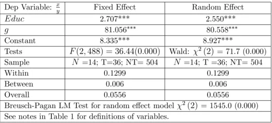
Tables 3 and 4 report static panel regressions of export share xy ;import share (m
y) on education share (Educ) and growth rate (g).
4 While both
models are signi…cant on the basis of F and 2 tests, the random e¤ect
model is recommended by the Breusch-Pagan LM test.5
Table 3: Static Panel Regression of Export Ratio on Education Spending Ratio and Growth Rate
Dep Variable: xy Fixed E¤ect Random E¤ect
Educ 2.707*** 2.550*** g 81.056 80.558 Constant 8.335*** 8.927*** Tests F(2;488) = 36:44(0:000) Wald: 2(2) = 71.7 (0.000) Sample N =14; T=36; NT= 504 N =14; T =36; NT= 504 Within 0.1299 0.1299 Between 0.006 0.006 Overall 0.0556 0.0556
Breusch-Pagan LM Test for random e¤ect model 2(2) = 1545.0 (0.000) See notes in Table 1 for de…nitions of variables.
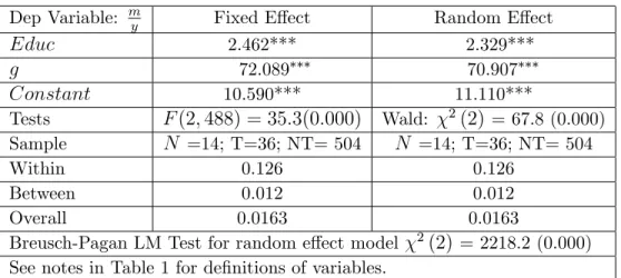
We …nd clear evidence of positive impacts of education spending ratio
(Educ) and growth rates (g) on ratios of exports x
y and imports
m y .
Fixed and random e¤ect estimates presented in Tables 3 and 4 provide strong empirical evidence for the central hypothesis of this paper that countries that
4These regression results are robust on the grounds of stationarity and cointegration
criteria. We have performed common panel unit root tests and Pedroni’s (1999) panel cointegration tests involving my; xy; Educand gand found a long run relationship. These results are not reported here for brevity but available from the authors upon request.
5It is important to note that the panel regression results reported here only show a long
run relationship between openness, education and growth. Many factors could contribute to an endogenous long run relationship between these three variables. In this paper, we focus on cognitive skills.
spend more on education and grow faster are more open. The Breusch-Pagan LM test suggests that random e¤ect model is more appropriate although there is little di¤erence in the estimates between these two models.
Table 4: Static Panel Regression of Import Ratio on Education Spending Ratio and Growth Rate
Dep Variable: my Fixed E¤ect Random E¤ect
Educ 2.462*** 2.329*** g 72.089 70.907 Constant 10.590*** 11.110*** Tests F(2;488) = 35:3(0:000) Wald: 2(2) = 67.8 (0.000) Sample N =14; T=36; NT= 504 N =14; T=36; NT= 504 Within 0.126 0.126 Between 0.012 0.012 Overall 0.0163 0.0163
Breusch-Pagan LM Test for random e¤ect model 2(2) = 2218.2 (0.000) See notes in Table 1 for de…nitions of variables.
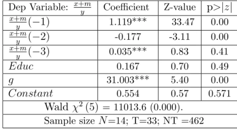
In these panel regressions, there is a potential problem of endogeneity of regressors due to correlation of the unobserved panel level e¤ects with
the lagged dependent variables. This could lead to inconsistency of
esti-mates. Arellano and Bover (1995) and Blundell and Bond (1998) employ
a GMM method to remove such inconsistency which is appropriate for a large panel and fewer periods. Estimations based on Blundell-Bond (1998)
system method are reported in Tables 5 and 6. Both Arellano-Bover and
Blundell-Bond estimation methods perform better than the Arellano-Bond
(1991) estimator for our sample. A robust and signi…cant dynamic panel
relationship holds between the overall trade share and growth. Although ed-ucation spending ratio has a positive sign as expected, it is not statistically signi…cant. This issue could be investigated further as richer and better data sets become available.
Table 5: Dynamic Panel Regression of Trade Ratio on Education Spending Ratio and Growth Rate: Arellano-Bover/Blundell-Bond Estimation
Dep Variable: x+ym Coe¢ cient Z-value p>jzj
x+m y ( 1) 1.119*** 33.47 0.00 x+m y ( 2) -0.177 -3.11 0.00 x+m y ( 3) 0.035*** 0.83 0.41 Educ 0.167 0.70 0.49 g 31.003*** 5.40 0.00 Constant 0.554 0.57 0.571 Wald 2(5) = 11013.6 (0.000). Sample sizeN=14; T=33; NT =462
Table 6: Dynamic Panel Regression of Import Ratio on Education Spending Ratio and Growth Rate: Arellano-Bover/Blundell-Bond Estimation
Dep Variable: my Coe¢ cient Z-value p>jzj
m y( 1) 1.151*** 34.33 0.00 m y( 2) -0.338*** -5.89 0.00 m y( 3) -0.124*** 2.94 0.00 Educ 0.093 0.71 0.48 g 15.226*** 5.00 0.00 Constant 1.135** 2.11 0.04 Wald 2(5)= 7933.6 (0.000) Sample sizeN=14; T=33; NT =462
2.3
Is cognitive skill a driver of the cross-country
rela-tionship between openness, education and growth?
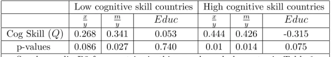
The central hypothesis of this paper is that the cross-country relationship between openness, education and growth is attributed to cross-country vari-ation of a common fundamental which is cognitive skill. To see the empirical plausibility of such a hypothesis we compute the cross-country correlation and regression of export, import and education shares on cognitive skill which are reported in Tables 7 and 8. The high cognitive skill of pupils, measured
by international test scores in mathematics and science could result from numerous factors including better quality of schooling, as well as education
subsidy.6 Using cross section data set from Hanushek and Woessmann (2008)
for cognitive skills for 2006 we compute the cross-country correlations of cog-nitive skills with export, import and education shares for all 75 countries and selectively for low and high cognitive skill countries as reported in Table 7.
High-cognitive skill countries with a score more than 4.803 tend to spend less time on education and have a higher trade share.
Table 7: Pearson correlation coe¢ cients among cognitive skill, imports, exports and education shares
Low cognitive skill countries High cognitive skill countries
x y m y Educ x y m y Educ Cog Skill(Q) 0.268 0.341 0.053 0.444 0.426 -0.315 p-values 0.086 0.027 0.740 0.01 0.014 0.075
See Appendix B2 for countries in this sample and also notes in Table 1
The data for cognitive skill are limited and only available for a single year, 2006, from Hanushek and Woessmann (2008). Thus standard Granger causality tests are not possible. We thus explore the causal relation between cognitive skills and the above variables using a cross section regression of av-erages of growth rate (g), education ratios (Educ) imports my and exports
shares x
y on cognitive skill as a right hand side variable. The e¤ects of
cognitive skills on openness and growth are found to be positive and signif-icant at the 5% level as shown in Table 8. The coe¢ cient of cognitive skill on education spending ratio regression is negative but not found statistically signi…cant at the 5% level. However, when splitting the sample between low cognitive skill and high cognitive skills (using the median as the cut-o¤ point), a positive relationship, although not statistically signi…cant, emerges
6Hanushek and Woessmann (2008) dataset contains 75 countries. They compute the
cognitive skills average of each country based on PISA test scores in mathematics and science. We thank them for providing us this data.
between these two variables for low cognitive-skill countries.
Reverse regressions of cognitive skill on growth or openness measures (not reported here for brevity) are not found to be statistically signi…cant which tends to suggest that cognitive skill is the driving force in determining the three important macroeconomic variables. Although such static regressions do not necessarily lead us to conclude anything about the causal ordering, it provides enough motivation for our endogenous growth model where cogni-tive skill is a driver of the cross-country relationship between openness and growth.
Table 8: Regression of growth rate, export and import shares on congnitive skills
g Educ Educ_low Educ_high xy my
Constant -18.95 18.62** 3.35 16.88** -558.0* -470.8* Cognitive-skill (Q) 4.50*** -2.76 0.11 -2.41 120.0** 102.0** R2 0.18 0.10 0.02 0.08 0.20 0.18 F 4.2** 3.4* 0.05 2.86 7.7*** 6.9** DW 2.6 1.75 2.04 1.71 2.70 2.60 N 33 33 41 34 33 33
See notes on Table 1. Educ_lowandEduc_highstand for education ratios of low
and high cognitive skill countries respectively.
The development facts emerging from these panel correlation and regres-sion analyses can be summarized as follows. First, there is a signi…cant cross-country positive correlation between trade openness and educational
investment. Second, countries with a higher cognitive skill index tend to
grow faster and are more open on the trade front. These correlation and re-gression results are used to motivate the formulation of an endogenous growth model in the next section. The central object of this growth modelling is to understand the linkage between cognitive skill, openness and education by cross country variation of cognitive skills alone.
3
The Model
The model is a small open economy adaptation of the Lucas-Uzawa (Lucas,
1988) model. There are two sectors, goods and education. We view the
problem from the perspective of a representative small open economy in a
global environment. The home country produces the output in the goods
sector (yt) with physical capital (kt) and home grown intangible or human
capital (ht). The human capital evolves following the linear technology:
ht+1 = (1 h)ht+Qtht (1)
where h2(0;1)is the rate of depreciation7 andQtis a crucial human capital
fundamental called cognitive skills of the home country’s population. Given the current level of human capital (ht), the human capital achieved in the
following period will be greater if the cognitive skills, Qt are higher. The
introduction of this cognitive skills variable is motivated by the recent work of
Hanushek and Woessmann (2008).8 By cognitive skill, we mean the learning
ability of pupils. This learning ability could depend partly on parent’s and pupil’s schooling e¤orts. We posit the following technology for the cognitive skill.
Qt=AHt:lHt (2)
where >0and lHt is the fraction of raw labour time (inelastically supplied
at unity) allocated to schooling. We do not impose any restriction such as diminishing returns to schooling e¤orts in augmenting cognitive skill as the nature of returns to scale in human capital is a debatable question. In fact, increasing returns to cognitive skill are quite plausible ( exceeding unity)
7Alternatively(1
h)could be thought of as the degree of intergenerational
transmis-sion of knowledge as in Bandyopadhyay and Basu (2005).
8Basu and Guariglia (2008) also use the same human capital investment technology to
if there is family based externality.9 For example, in addition to parent’s
own e¤ort, the child can additionally bene…t if other family members such as grandparents could spend time on the child’s education. This is akin to what Friedman (1962) calls "neighbourhood e¤ect" of education in a free society.
In our calibration exercise, we allow a range of variation of around the
baseline value of unity.10 The variableA
Ht is an exogenous educational total
factor productivity (TFP) variable that depends on a host of institutional and public policy factors including positive externality and social returns of public spending on education.11
Final goods (yt) are produced with the help of human and physical capital
via the Cobb-Douglas production technology:
yt =AGtkt (lGtht)1 (3)
with 0 < < 1: The variable AGt is the date t exogenous total factor
productivity (TFP) in the goods sector, andlGt (= 1 lHt) is the fraction of
raw labour directed to the goods sector production.
We assume the following stationary stochastic processes for these two TFP shocks around the steady state:
AGt AG = G(AGt 1 AG) + Gt (4)
AHt AH = H(AHt 1 AH) + Ht (5)
9 For example, Romer (1986) speci…es a production technology with increasing returns
to knowledge capital.
10When equals unity, the human capital technology reduces to Lucas (1988) technology
which we treat as our baseline for calibration. In our sensitivity analysis, we allow to range from 0.98 to 1.02.
11We abstract from public policy and institutional factors that could in‡uence public
policy. Basu and Bhattarai (2010) explore a model where the cognitive skill could depend on the public spending on education. Basu (2009) argues that malnutrition could impair pupil’s learning ability.
where AG and AH are the steady state TFP of the goods and education
sectors. Autocorrelation coe¢ cients G and H are positive fractions and
G t
and Ht are white noises.
Final goods are used for consumption (ct), domestic investment (idt) and
export (xt). The resource constraint facing the home country is:
ct+idt +xt=yt (6)
The home country imports raw materials (rmt)at a …xed pricepk: Examples
of these imported raw materials are machine tools, technology blueprints, patents etc.
Investment goods (ik
t) are produced combining domestic nontraded
in-vestment goods (idt) and imported raw materials (rmt) in …xed proportions
using the following Leontief production function:
ikt = min idt; rmt (7)
which means that ik
t =idt =rmt along an e¢ cient production frontier.12
The domestic physical capital stock evolves following the standard linear depreciation rule:
kt+1 = (1 k)kt+ikt (8)
The home country …nances these imported raw materials by a combina-tion of export and foreign borrowing (bt) at a …xed world interest rate, r .
The current account equation is given by:
12An example could help to motivate such a technological environment. Suppose the
home country produces an extra computer (ik
t ). It requires a home produced mother board
(id
t ) and an imported co-processor (rmt ). Thus an increase in investment in physical
capital necessitates an equi-proportionate increase in imported raw materials/intermediate input.
xt+bt+1 = (1 +r )bt+pkrmt (9)
The home country faces a borrowing constraint. The amount that it can borrow in the international market is constrained by the current capital stock of home country, which means13:
bt kt (10)
The time-line is as follows. At datet, the state of the economy is charac-terized bykt,htandbt. The home country after realizing the TFP shocks, Gt
and Ht , makes decisions about goods production (yt), schooling time (lHt),
exports (xt); external borrowing (bt+1) and consumption (ct) which
maxi-mizes the following expected utility functional:
E0 1 X t=0 t U(ct) subject to (1) through (10).
Assuming that the borrowing constraint binds, plugging (7), (8) , (9) and (10) into (6) one gets the combined resource constraint:
ct+pkkt+1 f(1 +pk)(1 k) 1 r gkt=yt: (11)
13Such a borrowing constraint can be motivated as follows. While setting a credit
limit, the external lending agency (say the World Bank) takes into consideration the long run growth prospect of the home country. Thus in principle, the borrowing limit is determined by the present value of the future stream of output of the home country. Since along a balanced growth path, home country’s output/capital ratio is a constant, the borrowing limit is thus proportional to the capital stock,kt: We assume here an exogenous
borrowing constraint. Such a borrowing constraint can be rationalized by following the lines of reasoning of Eaton and Gersovitz (1981) who show that the borrowing limit is the minimum of the amount that a country wishes to borrow and the credit ceiling determined by the lender based on their perception of default risk of the sovereign country.
4
Balanced Growth Properties
Hereafter we specialize to a logarithmic utility function, U(ct) = lnct; to
analyze the long run and short run properties of the model. In order to
focus on the long run properties of the model, we assume also that the two
productivity variables, AGt and AHt are …xed at the stationary levels AG
and AH:
The balanced growth equations for the key macroeconomic variables are as follows. The Appendix A.2 shows the details of the derivation.
Growth Rate: 1 +g = ht+1 ht = kt+1 kt = ct+1 ct = [1 h+AHlH 1(lH + lG)] (12) Export Share in GDP: xt GDPt = (1 h+AH)(p k 1) + (1 +r ) (1 k)pk M P K : lG lG+ (1 )lH (13) Import Share in GDP:
Denote the import bill of raw materials asmt. By de…nition,mt=pk:rmt:
Thus, import share in GDP is given by:
mt GDPt = p k f (1 +AH h) (1 k)g M P K : lG lG+ (1 )lH (14)
where M P K denotes the marginal product of physical capital.
Education Share in GDP:
Educ= (1 )lH
lG+ (1 )lH
(15) where GDPat date t is de…ned as:
GDPt = tyt+ tQtht (16)
Few clari…cations about these equations are in order. Equation (12)
is the balanced growth rate which depends in a quite standard way on the relative time allocations, the productivity parameters entering the human
capital technology (1) and the subjective discount factor : Export and
im-port shares in (13) and (14) depend on the balanced growth properties of the model and thus they depend on the same set of parameters as well as the goods sector technology coming through the marginal product of capital term. The share of education in GDP in (15) is carefully computed by tak-ing into account that the GDP consists of …nal goods and education services which are produced in two di¤erent sectors. These two items have di¤erent shadow prices which are proportional to the marginal costs of diverting re-sources from one sector to the another. While computing the GDP one needs to multiply each item by its respective shadow prices which are the relevant Lagrange multipliers. This explains the GDP equation (16).
4.1
Comparative Statics and Simulation
The primary purpose of this section is to understand how the steady state balanced growth rate (g), openness (measured by ((x+m)=GDP) and educa-tion share (Educ) respond to changes in the long run cognitive skills (Q). It may be noted from (2) that cognitive skill is endogenous because it depends
on the time allocated to the education sector, lH. How this time spent on
schooling in‡uences cognitive skill Q depends on the two schooling
technol-ogy parameters, namely AH and ; which are our main focus of attention
in this section. Countries may di¤er in these two cognitive skill parameters which could give rise to cross country dispersion in growth, education share
and openness.14 Such a comparative statics analysis could give useful insights
why high-cognitive-skill countries invest more in schooling, grow faster and are more open, which is the central question in this paper.
An inspection of the growth equation, (12), the export and import share equations (13) and (14), the education share (15) equation reveals that these two cognitive skill parameters appear either explicitly or implicitly in all
these equations. We start from a baseline case = 1 for which we have
tractable analytical results. We have the following proposition.
Proposition 1 If = 1, along the balanced growth path, the following results hold: lH = (1 )(1 h) AH (17) Educ= (1 )lH 1 lH (18) k h = 2 4 AG pk(1 h+AH) + (1 +r ) (1 k)(1 +pk) 3 5 1 1 (1 lH) (19) M P K =pk(1 h+AH) + (1 +r ) (1 k)(1 +pk) (20)
Proof: Appendix A.3.
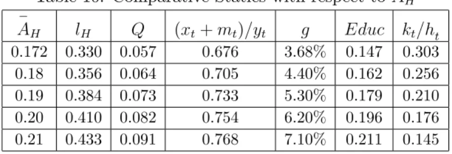
A sharp implication of Proposition 1 is that a long run increase in cogni-tive skill (AH) raises the time allocation (lH) to the education sector and a
higher education share (Educ). This results in a higher stock of human cap-ital which depresses the ratio of physical to human capcap-ital ratio (k=h). Thus it raises the marginal product of capital (M P K). Because of nonlinearity,
14It is needless to mention here that many factors besides cognitive skills could give
rise to cross country variation in these three key variables. Our focus in this paper is on cognitive skill.
it is not analytically obvious how export and import shares in equations (13)
and (14) respond to a change in AH. We, therefore, resort to a numerical
simulation based on a calibrated version of this model. This baseline model will also be used in the next section for performing short run analysis.
There are nine parameters, AG, AH, pk, r , , , h, k, and which
describe the preferences, technology and accumulation processes in the
econ-omy. Parameters and are …xed at the conventional levels as in many
studies including Prescott (1986). The second moment parameters for the
two forcing processes AGt and AHt are also …xed at levels as in Ma¤ezzoli
(2000). The world interest rate r is …xed at 4% in line with the Bank of
England estimate.15 The depreciation rates k and h are …xed at the values
calibrated by Ma¤ezzoli (2000) who also has a two sector growth model
sim-ilar to ours. The goods sector TFP scale parameter AG is …xed at 1.2 as in
Basu et al. (2011). The human capital productivity scale parameter AH is
…xed to target a 3.67% median growth rate for our sample of 182 countries. The relative price of capitalpk is …xed at 6 to target the median trade share
of 71.27% for our sample of 186 countries. The cognitive skill parameter
is …xed at 1 on par with Proposition 1. Such a value of gives rise to a 2:1
time allocation between goods and education sectors which is consistent with other studies including Benk et al. (2009) and Basu et al. (2009). Table 9 reports the baseline values of these parameters.
Table 9: Baseline Parameters
pk A
H AG r h k G H G H
0.65 6.00 0.172 1.2 0.04 0.9 0.020 0.011 1.00 0.962 0.962 0.032 0.032
Table 10 reports the comparative statics of the steady state variables
with respect to a small change in AH. In line with proposition 1, a higher
AH induces agents to invest more time to schooling and less time in goods
Table 10: Comparative Statics with respect to AH AH lH Q (xt+mt)=yt g Educ kt=ht 0.172 0.330 0.057 0.676 3.68% 0.147 0.303 0.18 0.356 0.064 0.705 4.40% 0.162 0.256 0.19 0.384 0.073 0.733 5.30% 0.179 0.210 0.20 0.410 0.082 0.754 6.20% 0.196 0.176 0.21 0.433 0.091 0.768 7.10% 0.211 0.145
production because education has a higher marginal return vis-a-vis goods production. As agents transfer resources away from goods to education, the physical to human capital ratio falls (last column of the Table 10), and growth
rate rises. Such a scarcity of physical capital raises the marginal product
of physical capital (due to diminishing returns to factor proportion). Recall from (7) that physical capital is produced with the aid of home grown in-vestment goods, id
t and the imported raw materialsrmt in …xed proportion.
Since the home country has the option to …nance the purchase of raw ma-terials through the current account, it will take advantage of it by raising its export and import shares. Thus the country becomes more open on the trade front. The bottom-line is that as a consequence of higherAH, the home
country invests more in education, its growth rises and its trade share also increases.
Our baseline model reproduces an education share of GDP (14%) which is a bit higher compared to the median 4.04 % of education spending ratio (Educ) for our sample of countries as reported in Table 1. It is important to understand that a 4.04% median public spending ratio is an underestimate of investment spending on schooling in the context of our model where an aggregative household spends time and resources in schooling. There are at least two reasons why the o¢ cial data on public spending on education may not re‡ect the steady state education spending ratio based on our aggregative model. First, the education expenditure data only refer to public spending
on education and do not include private spending on education. Whatever limited cross-country evidence is available for private spending on education,
it suggests that it is substantial. Armellini and Basu (2009) estimate the
ratio of household to total spending on education for a limited sample of 34
countries and …nd that the mean ratio is about 20%. In addition, Johnes
(1993) compiles the same estimate for 10 major countries and …nds that it ranges from 3.5% to 50.3%. Second, the education expenditure in our model is directly proportional to time to schooling lHt which basically re‡ects the
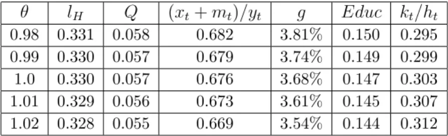
opportunity cost of schooling due to the lost wages at work. For example, parents might spend a signi…cant amount of time in tutoring their children which means a lot of schooling e¤orts. Goryan, Hurst, Kearney (2008) use the time use surveys for several countries to report that parents use about 25 percent of active time on average (8 hours a week) to take care and educate their children. In a similar vein, Blankenau and Camera (2009) argue that schooling attendance may be the same across countries but e¤orts may di¤er. Table 11 reports the marginal e¤ects of an increase in the value of below or above unity. Since is the elasticity of cognitive skill with respect to time
spent on schooling, a higher means that the agent can increase the cognitive
skills of his child by adding less time to schooling. The time freed up can be
dedicated to goods production to produce more consumables. This lowers
the share of education spending in GDP. A larger lowers the cognitive
skills Q as parents devote less time to schooling of kids and this sharply
lowers the growth rate. Since output decreases, a slight fall in openness
results as the economy produces less output and can export less. Overall,
growth, education share and openness decrease as increases.
To sum up: If countries di¤er in terms of the long run skills Q due to
either di¤erences AH or a positive cross country correlation between long
Table 11: Comparative Statics with respect to lH Q (xt+mt)=yt g Educ kt=ht 0.98 0.331 0.058 0.682 3.81% 0.150 0.295 0.99 0.330 0.057 0.679 3.74% 0.149 0.299 1.0 0.330 0.057 0.676 3.68% 0.147 0.303 1.01 0.329 0.056 0.673 3.61% 0.145 0.307 1.02 0.328 0.055 0.669 3.54% 0.144 0.312
4.2
Role of TFP in the Goods Sector
What is the role of the goods sector productivity, AG, in determining the
same correlation? It is straightforward to verify from Proposition 1 and
(13) and (14) that this steady state TFP has no e¤ects on balanced growth,
education share and trade shares because M P K is independent of AG (see
equation (20)). This basically means that a rise in AG is o¤set by a rise in
(k=h) to keep the M P K constant. This intuition is con…rmed in Table 12.
Thus in our model, the long run cross country correlation between openness and education is driven by cognitive skill alone.
Table 12: Comparative Statics with respect to AG
AG lH Q (xt+mt)=yt g Educ kt=ht 1.2 0.330 0.057 0.676 3.68% 0.147 0.303 1.3 0.330 0.057 0.676 3.68% 0.147 0.381 1.4 0.330 0.057 0.676 3.68% 0.147 0.471 1.5 0.330 0.057 0.676 3.68% 0.147 0.574 1.6 0.330 0.057 0.676 3.68% 0.147 0.690
5
Short Run Dynamics
Until now we only analyzed the long run properties of the model. Such a long run analysis can be motivated by cross-country comparisons of
vari-ous long run averages such as average growth, trade share and education share. The underlying assumption here is that each country is in di¤erent long run steady states and the research question is to understand what drives
the cross-country dispersion in steady states? There are two productivity
fundamentals, AG and AH in goods and education sectors among which we
identify the latter as the crucial determinant of the cross country dispersion of growth, education share and trade share. However, such a long run analy-sis cannot re‡ect how a country can respond to shocks to its productivity
fundamentals, AG and AH. Shocks to these fundamentals can arise due
to changes in tax policy. For example, a one-time education subsidy in the form of hiring high quality teachers can have an impact upon the cognitive skill, AH: On the other hand, institution of a temporary capital income tax
could hurt the goods sector productivity,AG. Analysis of this kind of
within-country response to shocks necessitates a short run analysis to which we turn now.
5.1
Impulse Responses
Appendix A.4 summarizes the relevant short run equations. There are eight relevant endogenous variables, namely,lHt,xt=yt,mt=yt,Educt, cat=yt,kt=ht,
Qt, andyt+1=ytand two exogenous variables, AHt andAGt:Among these
en-dogenous variables, onlykt=htis predetermined. The impulse response
analy-sis is based on log-linearized deviations of these variables from the steady state. Since this is a model of endogenous growth, the log-linearization is done around the balanced growth path described earlier. Figures 2 and 3 represent the impulse responses of various endogenous variables with respect
to shocks to TFP in each sector, namely Gt and
H
t based on (4) and (5)
given the baseline parameters in Table 9.16 In response to a positive shock
to Gt , more time is devoted to goods production and less to schooling. This
16 A variant of the algorithm of Blanchard and Kahn (1980) is used to plot the impulse
makes educational investment fall. Lower schooling e¤ort also lowers the cog-nitive skills. Since output growth rate depends on schooling e¤ort directly (see (A.25)), the growth rate also falls. This loss of output depresses the home country’s export share. On the other hand, as the human capital base decreases due to less time to schooling, the physical to human capital ratio (k=h)rises. This necessitates more import of raw materials due to the …xed coe¢ cient technology (7). The current account turns into a de…cit while the total trade share GDPx+m increases slightly as imports increase more than the loss of exports. 20 40 60 0 0.01 0.02 k/h 20 40 60 -0.01 0 0.01 lh 20 40 60 -2 0 2x 10 -3 g 20 40 60 -5 0 5x 10 -3 educ 20 40 60 -0.02 0 0.02 x/y 20 40 60 -0.02 0 0.02 m/y 20 40 60 -0.05 0 0.05 ca/y 20 40 60 -5 0 5x 10 -3(x+m)/y 20 40 60 -2 0 2x 10 -3 Q
Figure 2: Impulse responses with respect to Ag
In response to a cognitive skill shock, Ht ; the impulse responses behave di¤erently. Agents devote more time to schooling and less time to production of …nal goods. This raises output growth rate, educational share and cogni-tive skills. As GDP grows,the home country exports more. Imports initially drop as the country invests more resources in the education sector. However, the consequent rise in the marginal product of capital induces more domestic investment. The home country then requires to import more raw materials
20 40 60 -0.2 -0.1 0 k/h 20 40 60 0 0.1 0.2 lh 20 40 60 0 0.02 0.04 g 20 40 60 0 0.05 0.1 educ 20 40 60 0 0.2 0.4 x/y 20 40 60 -0.1 0 0.1 m/y 20 40 60 -0.5 0 0.5 ca/y 20 40 60 0 0.1 0.2 (x+m)/y 20 40 60 0 0.02 0.04 Q
Figure 3: Impulse responses with respect to Ah
to produce more investment goods using the …xed coe¢ cient technology (7). Overall, the current account turns into surplus. The openness measured by overall trade share increases.
The analysis of the transitional dynamics vividly illustrates that the short run e¤ects of these two types of productivity shocks have very di¤erent im-plications for the short run correlations between growth, openness and edu-cation. The short run correlation between growth, openness and education depends on which shock is predominant. If the predominant shock is TFP in goods sector, growth correlates positively with cognitive skill and educa-tion, while it correlates negatively with openness. Moreover, openness and education correlate negatively. On the other hand, if the predominant shock arises from the education technology (which we call cognitive skill), growth, openness and education share tend to correlate positively .17
17The variance decomposition of these two orthogonalized shocks, G
t; Ht suggests that
the latter accounts about 99% of the variation of relevant endogenous variables. Thus short run analysis also points to the direction that the shocks to education technology could be an important driver for growth, openness and education.
6
Conclusion
A plethora of literature exists about the relationship between openness and
growth. There is also a voluminous literature on education and growth.
However, less is known about the fundamentals driving openness, education and growth. The motivation for this study comes from the cross-country evidence that cognitive skill powerfully connects trade openness and educa-tional spending across countries. We construct an open economy endogenous growth model in the tradition of Lucas (1988) to understand this relationship. The time allocation between goods production and schooling in the spirit of Becker (1975) is an essential ingredient of human capital growth. Our model identi…es cognitive skill measured by international test scores in and science that enhances the productivity of human capital. This cognitive skill is a crucial driver of the cross- country relationship between education and trade openness. In terms of our endogenous growth model, we demonstrate that the cross-country di¤erences in cognitive skill play a central role in determin-ing the cross-country correlation between trade share and education share. This corroborates the development facts outlined in the paper that countries with higher cognitive skill grow faster, are more open and spend more on education.
Our model is the …rst in the literature showing explicitly the connection between cognitive skill, growth and trade openness. It is of course true that several factors besides cognitive skill are important determinants of growth, openness and education. For example, degree of democracy, trade and
non-trade barriers, exchange rate volatilities could matter for openness. An
evaluation of these factors on openness and growth in itself can be an agenda for future research. A useful extension of our work will also be to bring skill di¤erences in technology suggested by Epifani and Gancia (2008) and explore the implications for skill premium in the context of endogenous growth.
References
[1] Arellano, M., and S. Bond (1991), ‘Some tests of speci…cation for panel data: Monte Carlo evidence and an application to employment
equa-tions’, Review of Economic Studies 58, 277–297.
[2] Arellano, M., and O. Bover (1995) ‘Another look at the instrumental
variable estimation of error-components models’, Journal of
Economet-rics 68, 29–51.
[3] Armellini, M and P. Basu (2010), ‘Altruism, Education and Growth’, SSRN working paper.
[4] Bandyopadyay D. and P. Basu (2005), ‘What drives the cross country
growth and inequality correlations?’ Canadian Journal of Economics,
38,4,1272-1297, November.
[5] Barro, R. J.(1991), ‘Economic Growth in Cross Section of Countries’,
Quarterly Journal of Economics, 106, May, 407-433.
[6] Basu, P. (2009), ‘Too Hungry to Read: Is an Education Subsidy a
Mis-guided Policy for Development’, in the Handbook of Research in Cost
Bene…t Analysis, Edward Elgar, Cheltenham, UK, 335-372.
[7] Basu, P. and K. Bhattarai (2010), ‘Government Bias in Education,
Schooling Attainment and Growth’, Mimeo.
[8] Basu, P. and A. Guariglia (2008), ‘Does low education delay structural
transformation’, Southern Economic Journal, 75,1, 104-127.
[9] Basu, P., M. Gillman, and J. Pearlman (2009), ‘In‡ation, Human Cap-ital and Tobin’s q’, Mimeo.
[10] Becker, G.S. (1975), Human Capital. University of Chicago Press,
[11] Benk, S, M. Gillman, M. Kejak (2009), ‘US Volatility Cycles of Output and In‡ation, 1919-2004: A Money and Banking Approach to a Puzzle,’
CEPR Discussion Paper, No. 7150.
[12] Bils M., Klenow P.J. (2000), ‘Does Schooling Cause Growth?’American
Economic Review, 90, 5,Dec.,1160-1183.
[13] Blanchard, O. and C.M. Kahn (1980), ‘The Solution of Linear Di¤erence
Models under Rational Expectations’, Econometrica, 48, 5, July,
1305-1313.
[14] Blankenau, W & G. Camera (2009), ‘Public Spending on Education and the Incentives for Student Achievement’,Economica, 76,303,505-527, 07. [15] Blundell, R., and S. Bond (1998), ‘Initial conditions and moment
re-strictions in dynamic panel data models’, Journal of Econometrics, 87,
115–143.
[16] Cartiglia, F. (1997), ‘Credit constraints and human capital accumulation in the open economy’, Journal of International Economics, 43, 221,236. [17] Eaton J., M. Gersovitz (1981), ‘Debt with Potential Repudiation: Theo-retical and Empirical Analysis’,Review of Economic Studies, 48, 2,Apr., 289-309.
[18] Epifani, P. and G. Gancia (2008), ‘The Skill Bias of World Trade’,
Eco-nomic Journal, 118,July, 927-960.
[19] Friedman, M (1962), Capitalism and Freedom, The University of
Chicago Press.
[20] Galor, O. and A. Mountford (2008), ‘Trading Population for
Productiv-ity: Theory and Evidence’,Review of Economic Studies, 75, 1143-1179.
[21] Grossman, G.M. and E. Helpman (1990), ‘Comparative Advantage and
[22] Guryan J., E. Hurst, and M. Kearney (2008), ‘Parental Education and
Parental Time with Children’, Journal of Economic Perspectives, 22,
3,Summer, 23–46.
[23] Hanushek, E. A. and L. Woessmann (2008), ‘The Role of Cognitive Skills
in Economic Development’, Journal of Economic Literature,
46,3,607-668, September.
[24] Johnes, G (1993), The Economics of Education. The Macmillan Press,
London.
[25] Jorgenson, D. W. and B. Fraumeni (1992), ‘Investment in Education and
US Economic Growth’, Scandinavian Journal of Economics, 94,51-70.
[26] Julliard, M. (1996), ‘Dynare: A Program for the Resolution and Simu-lation of Dynamic Models with Forward Variables through the Use of a
Relaxation Algorithm’, CEPREMAP, Couverture Orange, 9602.
[27] Lucas, R.E. (1988), ‘On the Mechanics of Economic Development’,
Jour-nal of Monetary Economics, 22,1, 3-42.
[28] Ma¤ezzoli, M. (2000), ‘Human Capital and International Real Business
Cycles’, Review of Economic Dynamics, 3,137-165.
[29] Mankiw, N.G., D. Romer and D. N. Weil (1992), ‘Contribution to
the Empirics of Economic Growth’, Quarterly Journal of Economics,
107,407-437.
[30] Manning, R. (1982), ‘Trade, Education and Growth: The Small-Country
Case’, International Economic Review, 23,1,83-106.
[31] Parente, S.L. and E.C. Prescott (2002). Barriers to Riches. MIT Press,
[32] Pedroni, P. (1999), ‘Critical values for cointegration tests in
heteroge-neous panels with multiple regressors’, Oxford Bulletin of Economics
and Statistics, 61, Special Issue,653-670.
[33] Prescott, E.C. (1986), ‘Theory Ahead of Business Cycle Measurement’,
Federal Reserve Bank of Minneapolis, Quarterly Review, 10,9-22,Fall.
[34] Romer P. M. (1986), ‘Increasing Returns and Long-run Growth’,Journal
of Political Economy, 94, October,1002-1037.
A
Appendix
A.1
First Order Conditions
Let t; t be the Lagrange multipliers associated with the ‡ow budget
con-straint (6), human capital technology, (1). First order conditions are:
ct : tU0(ct) = t (A.1) kt+1 : tpk =Et t+1 AGt+1 kt+11(lGt+1ht+1)1 + (1 k)(1 +pk) (1 +r ) (A.2) ht+1 : t=Et t+1f1 h +AHt+1lHt+1)g (A.3) +Et t+1 AGt+1(1 )kt+1ht+1l 1 Gt+1 lGt : t(1 )AGtlGtktht1 tAHtht lHt1 = 0 (A.4)
A.2
Derivation of the Balanced Growth Equations
Along the balanced growth path, we assume that AGt =AG; AHt =AH: We
also exploit the fact that the raw labour allocation variables lGt and lHt are
stationary along the balanced growth path. Rewrite (A.3) as:
t t = t+1 t+1 : t+1 t : 1 h+AH:lH + t+1 t : AG(1 )lG1 : k h
Use (A.4) to substitute out t
t and noting that in the steady state t t is a constant, one gets:
1 = t+1 t : 1 h+AH:lH + t+1 t : t t : AG(1 )l1G : k h
Next use (A.1) to rewrite the above as:
1 +g = 1 h+AH:lH + t t : AG(1 )l1G : k h (A.5)
Finally note from (A.4) that
t t = AG(1 )lG : k h AH:lH 1
which upon substitution in (A.5) gives
Using (A.1), we get the following balanced growth rate (g) as follows: =>1 +g = ht+1 ht = kt+1 kt = ct+1 ct (A.6) Using (A.1), (A.3) and A.4) we get the balanced growth rate (12)
To get the export share equation (13) use (9), (8) and (10) which gives:
xt+kt+1 = (1 +r )kt+pk(kt+1 (1 k)kt)
Divide through by yt and use the fact that along a balanced growth
path kt=yt is a constant and for the Cobb-Douglas production function (3),
M P K = yt=kt; to get: xt yt = (1 h+AH)(p k 1) + (1 +r ) (1 k)pk M P K (A.7)
By de…nition, the export share in GDP is given by:
xt GDPt = xt yt : yt GDPt (A.8) Next use (16) and (A.4) to rewrite:
yt
GDPt
= lG
lG+ (1 )lH
(A.9) Plug (A.7) and (A.9) into (A.8) to get (13).
To get the import share equation (14), notice …rst that the share of import in GDP is given by: mt GDPt = p krm t yt : yt GDPt
which after using the fact thatrmt =ikt due to the …xed coe¢ cient production
mt GDPt = p k(k t+1 (1 k)kt) yt : yt GDPt (A.10) = pk kt+1 yt+1 (1 +g) (1 k) kt yt : yt GDPt = p k f(1 +g) (1 k)g M P K : yt GDPt which proves (14).
To derive the education share in GDP, note …rst that by de…nition:
Educ= tAHtlHtht
tyt+ tAHtlHtht
(A.11)
Plug (A.4) into (A.11) to substitute out t= t to obtain (15).
A.3
Proof of Proposition 1
When = 1;(12) reduces to
1 +g = (1 +AH h) (A.12)
Based on (1) one gets another balanced growth equation:
1 +g = 1 +lHAH h (A.13)
Equating (A.12) and (A.13) one obtains (17). Equation (18) follows from
(15) by setting = 1:
Next note that the following third balanced growth equation can be ob-tained from the Euler equation for physical capital (A.2).
1 +g =pk1 " AG l1G k h 1 + (1 k)(1 +pk) (1 +r ) # (A.14)
Equating (A.12) to (A.14) one can solve lG1 kh 1 which yields (19).
To get (20) simply observe thatM P K = y=kwhich is simplyAG l1G kh
1 :
Plugging the expression for (19) the result is immediate.//
A.4
Summary of Short-run Equations
De…ne
t=
lGt
lGt+ (1 )lHt
(A.15) The short run system is given by equations (A.16) to (A.25) are:
kt+1 ht+1 = t: pk(1 k)kht t +AGt( kt ht) l 1 Gt ct ht (1 +r ) kt ht f1 h+AHt(1 lGt) g (A.16) 1 =dft+1: AGt+1 hktt+1+1 1 l1Gt+1+ (1 k)(1 +pk) 1 r pk (A.17) 1 :l1Ht AGt Aht :lGt:(kt ht ) = dft+1 AGt+1 Aht+1 : 1:l1Ht+1lGt+1:(kt+1 ht+1 ) f1 h+AHt+1(1 lGt+1)g+AGt+1 kt+1 ht+1 l1Gt+1 (A.18) wheredft+1 is the discount factor given by
dft+1 = (ct=ht) (ct+1=ht+1) 1 (AHt+1(1 lGt+1) + 1 h) (A.19) Export and import share equations are given by:
xt GDPt = t:[1 +r pk(1 k)](kt=yt) (A.20) +(pk 1)(kt+1=yt+1)(AGt+1=AGt) kt+1=ht+1 kt=ht f 1 h+AHtlhtg: lGt+1 lGt 1 mt GDPt = t:pk " kt+1 yt+1 :AGt+1 AGt : kt+1=ht+1 kt=ht lGt+1 lGt 1 f1 h+AHtlhtg (1 k): kt yt # (A.21) The ratio of current account to GDP is de…ned as:
cat GDPt = xt yt mt yt : t (A.22)
The openness is de…ned as:
opent=
xt+mt
yt
: t (A.23)
The education share equation is given by:
Educt=
(1 )lHt
lGt+ (1 )lHt
(A.24) Finally the growth rate of output is given by:
yt+1 yt = AGt+1 AGt : AGt+1 AGt kt+1=ht+1 kt=ht f AHtlHt+ 1 hg: lGt+1 lGt 1 (A.25)
A.5
Outline of the Derivation of the Short-run
Equa-tions
Rewrite (6) as: kt+1 = (1 k)(1 +pk)kt+AGtkt(lGtht)1 ct (1 +r )kt pk (A.26)Dividing (A.26) by (1), one gets (A.16). (A.17) can be obtained by
combining (A.1),(A.2) and (10).
Use (A.3) and (A.4) to obtain (A.18).
The discount factor (A.19) is basically ct=ct+1. This can be rewritten as
f(ct=ht)=(ct+1=ht+1)g(ht+1=ht) 1: After using (1), one gets the
expres-sion for (A.19).
To obtain the export share equation (A.20) , use (10) and (9) to obtain:
xt= (1 +r )kt+ (pk 1)kt+1 pk(1 k)kt (A.27)
Divide through byyt and multiply by t as in (A.15) to obtain (A.20).
To get (A.21), use
mt yt = p k(k t+1 (1 k)kt) yt (A.28) which can be rewritten as:
mt yt =pk(kt+1 yt+1 :yt+1 yt (1 k) kt yt ) (A.29)
which after using the production function (3) and the human capital equation (1) together with (A.15) yields the expression (A.21).
The expression for the current account (A.22) follows by de…nition. The expression for (A.24) is the same as the steady state expression (1). The
expression for the growth rate in (A.25) follows from the use of the production function (3) and the human capital equation (1).
B
Data for the Empirical Analysis
B.1
Notes on data access and manipulations
Data Sources:
g : Growth rate of GDP (annual %) for 1960-2006, World Development Indicators, 2008.
Educ : Education expenditure (% of GNI) for 1960-2006, World Develop-ment Indicators, 2008.
x
y : Exports of goods and services (% of GDP) for 1960-2006, World
Devel-opment Indicators, 2008.
m
y : Imports of goods and services (% of GDP) for 1960-2006, World
Devel-opment Indicators, 2008.
x+m
y : Total trade (% of GDP), for 1960-2006, World Development
Indica-tors, 2008.
rm
y : Merchandise trade (% of GDP),as de…ned in the IMF’s DOTS , for
1960-2006, World Development Indicators, 2010.
Q : Cognitive skills of pupils re‡ects the quality of schooling measured by the PISA test scores in mathematics and science and taken from Hanushek and Woessmann (2008) for 2006.
Notes on data access and manipulations
1. The World Development Indicators-database was accessed from at: http://www.esds.ac.uk/international/.
2. For each of these variables, the time average is …rst computed for each coun-try over the period 1960-2006. Countries with missing data have a shorter
sample period. Then a cross country mean, median, skewness (indicating the di¤erence between mean and median) and the inter-quartile ranges are computed.
3. For many of these emerging countries, export ratios (xy) show up more than their GDP in the balance of payments account. For example, Singapore buys textiles in China and sells them in Europe; it buys high tech equipment from the US and sells to China. In both cases goods are not produced in Singapore but these are counted as exports of Singapore. This explains why export share in GDP can exceed unity in extremely open countries.
4. Data for education ratio (Educ) is not available for 11 countries: Aruba, Bosnia and Herzegovina, Macao, China, Micronesia, Fed. Sts., Montenegro, Palau, Serbia, Turkmenistan, United Arab Emirates, West Bank and Gaza, Yemen Rep. Countries such as Cayman Islands, Guam, Isle of Man, Marshall Islands, Mayotte, Monaco, Netherlands Antilles, San Marino, and Timor-Leste are dropped from computations because of missing data in more than two variables.
B.2
Countries in the Empirical Analysis
1. For Correlations: Algeria, Angola, Antigua and Barbuda, Argentina, Arme-nia, Australia, Austria, Azerbaijan, Bahamas, Bahrain, Bangladesh, Barbados, Belarus, Belgium, Belize, Benin, Bhutan, Bolivia, Bosnia and Herzegovina, Botswana, Brazil, Brunei Darussalam, Bulgaria, Burkina Faso, Burundi, Cambodia, Cameroon, Canada, Cape Verde, Central African Republic, Chad, Chile, China, Colombia, Comoros, Congo Dem. Rep., Congo Rep., Costa Rica, Cote d’Ivoire, Croatia, Cuba, Cyprus, Czech Re-public, Denmark, Djibouti, Dominica, Dominican ReRe-public, Ecuador, Egypt, Arab Rep., El Salvador, Equatorial Guinea, Eritrea, Estonia, Ethiopia, Fiji, Finland, France, Gabon, Gambia, Georgia, Germany, Ghana, Greece, Grenada, Guatemala, Guinea-Bissau, Guinea, Guyana, Haiti, Honduras, Hong Kong-China, Hungary, Iceland, India, Indonesia, Iran, Is-lamic Rep., Ireland, Israel, Italy, Jamaica, Japan, Jordan, Kazakhstan, Kenya, Korea, Rep., Kuwait, Kyrgyz Republic, Lao PDR, Latvia, Lebanon, Lesotho, Liberia, Libya, Lithuania, Luxembourg, Macao-China, Macedonia-FYR, Madagascar, Malawi, Malaysia, Maldives, Mali, Malta, Mauritania, Mauritius, Mexico, Micronesia-Fed. Sts., Moldova, Mongolia, Montenegro, Morocco, Mozambique, Myanmar, Namibia, Nepal, Netherlands, New Zealand, Nicaragua, Nigeria, Niger, Norway, Oman, Pakistan, Panama, Papua New Guinea, Paraguay, Peru, Philippines, Poland, Portugal, Qatar, Romania, Russian Federa-tion, Rwanda, Samoa, Saudi Arabia, Senegal, Serbia, Seychelles, Sierra Leone, Singapore, Slovak Republic, Slovenia, Solomon Islands, Somalia, South Africa, Spain, Sri Lanka, St. Kitts and Nevis, St. Lucia, St. Vincent and the Grenadines ,Sudan, Suriname, Swaziland, Sweden, Switzerland, Syrian Arab Republic, Tajikistan, Tanzania, Thailand, Togo, Tonga, Trinidad and Tobago, Tunisia, Turkey, Turkmenistan, Uganda, Ukraine,
United Arab Emirates, United Kingdom, United States, Uruguay, Uzbekistan, Vanuatu, Venezuela, Vietnam, West Bank and Gaza, Yemen Rep., Zambia, Zimbabwe.
2. For Cognitive Skill: Albania, Argentina, Armenia, Australia, Austria, Bahrain , Belgium, Botswana, Brazil, Bulgaria, Canada, Chile, China, Colombia, Cyprus, Czech Republic, Denmark, Egypt, Arab Rep., Estonia, Finland, France, Germany, Ghana, Greece, Hong Kong, China, Hungary, Iceland, India, Indonesia, Iran, Islamic Rep., Ireland, Israel, Italy, Japan, Jordan, Korea, Rep., Kuwait, Latvia, Lebanon, Lithuania, Luxembourg, Macao, China, Macedonia, FYR, Malaysia, Mexico, Moldova, Morocco, Netherlands, New Zealand, Nigeria, Norway, Peru, Philippines, Poland, Portugal, Romania, Russian Feder-ation, Saudi Arabia, Serbia, Singapore, Slovak Republic, Slovenia, South Africa, Spain, Swaziland, Sweden, Switzerland, Thailand, Tunisia, Turkey, United Kingdom, United States, Uruguay, Palestine, Zimbabwe.
3. For Panel Regression Models: Fourteen groups of countries used in panel regression are based on the World Development Indicators (2007). The o¢ cial data (available using Athens login from the www.esds.ac.uk/international/WDI) de…ne these categories (with our own notation for each category in parentheses) as follows:
1. World aggregate is average of all countries of the world (Wrld).
2. Low-income economies ( Linc) are those in which 2007 GNI per capita was $935 or less including Afghanistan, Bangladesh, Benin, Burkina Faso, Burundi, Cam-bodia, Central African Republic, Chad, Comoros, Congo, Dem. Rep., Côte d’Ivoire, Eritrea, Ethiopia, Gambia, The, Ghana, Guinea, Guinea-Bissau, Haiti, Kenya, Korea, Dem. Rep., Kyrgyz Republic, Lao PDR, Liberia, Madagascar, Malawi, Mali, Mauritania, Mozambique, Myanmar, Nepal, Niger, Nigeria, Pakistan, Papua New Guinea, Rwanda, São Tomé and Principe, Senegal, Sierra Leone, Solomon Islands, Somalia, Tajikistan, Tanzania, Togo, Uganda, Uzbekistan, Vietnam, Yemen, Rep., Zambia, Zimbabwe.
3. Middle-income economies (Minc) are those in which 2007 GNI per capita was between $936 and $11,455 including countries in: Lower middle income and Upper middle income groups.
4. Lower-middle-income (Lminc) economies are those in which 2007 GNI per capita was between $936 and $3,705 and include: Albania, Algeria, Angola, Armenia, Azerbai-jan, Bhutan, Bolivia, Bosnia and Herzegovina, Cameroon, Cape Verde, China, Colombia, Congo, Rep., Djibouti, Dominican Republic, Ecuador, Egypt, Arab Rep., El Salvador, Georgia, Guatemala, Guyana, Honduras, India, Indonesia, Iran, Islamic Rep., Iraq, Jor-dan, Kiribati, Lesotho, Macedonia, FYR, Maldives, Marshall Islands, Micronesia, Fed. Sts., Moldova, Mongolia, Morocco, Namibia, Nicaragua, Paraguay, Peru, Philippines, Samoa, Sri Lanka, Sudan, Swaziland, Syrian Arab Republic, Thailand, Timor-Leste, Tonga, Tunisia, Turkmenistan, Ukraine, Vanuatu, West Bank and Gaza.
5. Upper-middle-income economies (Upminc) are those in which 2007 GNI per capita was between $3,706 and $11,455 including: American Samoa, Argentina, Belarus, Belize, Botswana, Brazil, Bulgaria, Chile, Costa Rica, Croatia, Cuba, Dominica, Fiji, Gabon, Grenada, Jamaica, Kazakhstan, Latvia, Lebanon, Libya, Lithuania, Malaysia, Mauritius, Mayotte, Mexico, Montenegro, Palau, Panama, Poland, Romania, Russian Federation, Serbia, Seychelles, South Africa, St. Kitts and Nevis, St. Lucia, St. Vincent and the Grenadines, Suriname, Turkey, Uruguay, Venezuela, RB.
6. Low- and middle-income economies (lmdinc) are those in which 2007 GNI per capita was $11,455 or less and include the following country groups: East Asia & Paci…c, Europe & Central Asia, Latin America & Caribbean, Middle East & North Africa, South Asia and Sub-Saharan Africa.
7. East Asia and Paci…c regional aggregate (ASPC) includes: American Samoa, Cambodia, China, Fiji, Indonesia, Kiribati, Korea, Dem. Rep., Lao PDR, Malaysia, Marshall Islands, Micronesia, Fed. Sts., Mongolia, Myanmar, Palau, Papua New Guinea, Philippines, Samoa, Solomon Islands, Thailand, Timor-Leste, Tonga, Vanuatu, Vietnam.
8. Latin America and Caribbean regional aggregate (LTACA) includes Argentina, Belize, Bolivia, Brazil, Chile, Colombia, Costa Rica, Cuba, Dominica, Dominican
Re-public, Ecuador, El Salvador, Grenada, Guatemala, Guyana, Haiti, Honduras, Jamaica, Mexico, Nicaragua, Panama, Paraguay, Peru, St. Kitts and Nevis, St. Lucia, St. Vincent and the Grenadines, Suriname, Uruguay, Venezuela, RB.
9. Middle East and North Africa regional aggregate (MDEAST) includes: Algeria, Djibouti, Egypt, Arab Rep., Iran, Islamic Rep., Iraq, Jordan, Lebanon, Libya, Morocco, Syrian Arab Republic, Tunisia, West Bank and Gaza, Yemen, Rep.
10. South Asia (SAsia) economies include: Afghanistan, Bangladesh, Bhutan, In-dia, Maldives, Nepal, Pakistan, and Sri Lanka.
11. Sub-Saharan Africa (SSAFR) includes: Angola, Benin, Botswana, Burkina Faso, Burundi, Cameroon, Cape Verde, Central African Republic, Chad, Comoros, Congo, Dem. Rep., Congo, Rep., Côte d’Ivoire, Eritrea, Ethiopia, Gabon, Gambia, The, Ghana, Guinea, Guinea-Bissau, Kenya, Lesotho, Liberia, Madagascar, Malawi, Mali, Maurita-nia, Mauritius, Mayotte, Mozambique, Namibia, Niger, Nigeria, Rwanda, São Tomé and Principe, Senegal, Seychelles, Sierra Leone, Somalia, South Africa, Sudan, Swaziland, Tanzania, Togo, Uganda, Zambia, Zimbabwe.
12. High-income economies (Hiinc) are those in which 2007 GNI per capita was $11,456 or more and include: Australia, Austria, Belgium, Canada, Czech Republic, Den-mark, Finland, France, Germany, Greece, Hungary, Iceland, Ireland, Italy, Japan, Korea, Rep., Luxembourg, Netherlands, New Zealand, Norway, Portugal, Slovak Republic, Spain, Sweden, Switzerland, United Kingdom, United States.
13. High income non-OECD economies (HinOECD) are those in which 2007 GNI per capita was $11,456 or more and include: Andorra, Antigua and Barbuda, Aruba, Ba-hamas, The, Bahrain, Barbados, Bermuda, Brunei Darussalam, Cayman Islands, Channel Islands, Cyprus, Equatorial Guinea, Estonia, Faeroe Islands, French Polynesia, Green-land, Guam, Hong Kong, China, Isle of Man, Israel, Kuwait, Liechtenstein, Macao, China, Malta, Monaco, Netherlands Antilles, New Caledonia, Northern Mariana Islands, Oman, Puerto Rico, Qatar, San Marino, Saudi Arabia, Singapore, Slovenia, Trinidad and Tobago, United Arab Emirates, Virgin Islands (U.S.).
14. Heavily indebted poor countries (HIPC) include: Afghanistan, Benin, Bo-livia, Burkina Faso, Burundi, Cameroon, Central African Republic, Chad, Comoros, Congo, Dem. Rep., Congo, Rep., Côte d’Ivoire, Eritrea, Ethiopia, Gambia, The, Ghana, Guinea, Guinea-Bissau, Guyana, Haiti, Honduras, Kyrgyz Republic, Liberia, Madagascar, Malawi, Mali, Mauritania, Mozambique, Nepal, Nicaragua, Niger, Rwanda, São Tomé and Principe, Senegal, Sierra Leone, Somalia, Sudan, Tanzania, Togo, Uganda, Zambia.