HAL Id: hal-01781257
https://hal.archives-ouvertes.fr/hal-01781257v2
Submitted on 26 Oct 2019HAL is a multi-disciplinary open access archive for the deposit and dissemination of sci-entific research documents, whether they are pub-lished or not. The documents may come from teaching and research institutions in France or abroad, or from public or private research centers.
L’archive ouverte pluridisciplinaire HAL, est destinée au dépôt et à la diffusion de documents scientifiques de niveau recherche, publiés ou non, émanant des établissements d’enseignement et de recherche français ou étrangers, des laboratoires publics ou privés.
An Adaptive Parareal Algorithm
Yvon Maday, Olga Mula
To cite this version:
An Adaptive Parareal Algorithm
Y. Maday, O. MulaAbstract
In this paper, we consider the problem of accelerating the numerical simulation of time dependent problems by time domain decomposition. The available algorithms enabling such decompositions present severe efficiency limitations and are an obstacle for the solution of large scale and high dimensional problems. Our main contribution is the improvement of the parallel efficiency of the parareal in time method. The parareal method is based on combining predictions made by a numerically inexpensive solver (with coarse physics and/or coarse resolution) with corrections coming from an expensive solver (with high-fidelity physics and high resolution). At convergence, the parareal algorithm provides a solution that has the fine solver’s high-fidelity physics and high resolution In the classical version of parareal, the fine solver has a fixed high accuracy which is the major obstacle to achieve a competitive parallel efficiency. In this paper, we develop an adaptive variant of the algorithm that overcomes this obstacle. Thanks to this, the only remaining factor impacting performance becomes the cost of the coarse solver. We show both theoretically and in a numerical example that the parallel efficiency becomes very competitive when the cost of the coarse solver is small.
1
Introduction
Solving complex models with high accuracy and within a reasonable computing time has moti-vated the search for numerical schemes that exploit efficiently parallel computing architectures. In this paper, the model consists of a Partial Differential Equation (PDE) set on a domain
D. In this context, one of the main ideas to parallelize a simulation is to break the problem into subproblems defined over subdomains of a partition of D. The domain can potentially have high dimensionality and be composed of different variables like space, time, velocity or even more specific variables for some problems. While there exist algorithms with very good scalability properties for the decomposition of the spatial variable in elliptic and saddle-point problems (see [29] or [30] for an overview), the same cannot be said for the decomposition of time of even simple systems of ODEs. This is despite the fact that research on time domain decomposition is currently very active and has by now a history of at least 50 years (back to at least [28]) during which several algorithms have been explored (see [14] for an overview). As a consequence, time domain decomposition is to date only a secondary option when it comes to deciding what algorithm/method distributes the tasks in a parallel cluster.
The main goal of this work is to address this efficiency limitation in the framework of one particular scheme: the parareal in time algorithm. The method was first introduced in [19] and has been well accepted by the community because it is easily applicable to a relatively large spectrum of problems. (Some specific difficulties are nevertheless encountered on certain types of PDEs as reported in, e.g., [8, 12] for hyperbolic systems or [4, 7] for hamiltonian problems). Another ingredient for its success is that, even though its scalability properties are limited, they are in general competitive in comparison with other methods. Without entering into very specific details of the algorithm at this stage, we can summarize the procedure by saying that
we build iteratively a sequence to approximate the exact solution of the problem by a predictor-corrector algorithm. At every iteration, predictions are made by a solver which has to be as numerically inexpensive as possible since it is run on the full time interval. It usually involves coarse physics and/or coarse resolution. Corrections involve an expensive solver with high-fidelity physics and high resolution which is propagated in parallel over small time subdomains. In the classical version of parareal, the fine solver has a fixed high accuracy across all iterations. It is set to the one that we would use to solve the dynamics at the desired accuracy with a purely sequential solver. It is well-known that this point is the major obstacle to achieve better parallel efficiency. In this paper, we propose an adaptive variant where the accuracy of the fine solver is increased across the iterations. Our main goal is to show that this new point of view overcomes the obstacle of the cost of the fine solver and that the only remaining factor limiting high performance becomes the cost of the coarse solver. We refer to, e.g., [6] for contributions on the lowering of the cost of that coarse solver.
We present in section 2 the new adaptive point of view. This requires to formulate an ide-alized version of the parareal algorithm in an infinite dimensional function space where the fine propagations are replaced by the exact ones (section 2.2). Since this scheme is obviously not implementable in practice, we formulate a feasible “perturbed” version that involves approxi-mations of the exact propagations at increasing accuracy across the iterations (section 2.3). The accuracies are tightened in such a way that the feasible adaptive algorithm converges at the same rate as the ideal one and with a near-minimal numerical cost. The identified tolerances involve quantities that are difficult to estimate in practice. In addition, they may not be optimal because they are derived from a theoretical convergence analysis based on abstract conditions for the coarse and fine solvers. We bridge this gap between theory and actual implementation by proposing practical guidelines to set these tolerances. We next explain in section 2.4 how the new formulation invites to use adaptive schemes not only in the time variable, but also in other variables that may be involved in the dynamics. The performance of the algorithm could also be enhanced by re-using informations from previous iterations in order to limit the cost of internal solvers. The techniques for this will strongly depend on the nature of the specific prob-lem. We discuss common situations in Appendix A. We close section 2.5 by listing the main advantages of the new framework and how the classical parareal paradigm can be formulated with the optics of the new standpoint.
The parallel performance of the adaptive scheme is difficult to predict a priori but in section 3 we carry a discussion where we show that it will always be superior to the classical approach. In the idealized situation where the cost of the coarse solver and communication delays are negligible, we show that the algorithm would exhibit a very high parallel efficiency.
Finally, in section 4, we illustrate the performance of the algorithm in a numerical example: the Brusselator system. It is a stiff ODE system which is challenging because it does not allow to use a very inexpensive coarse solver. We show that the adaptive parareal algorithm systematically performs around 2.5 times better than the classical one. In addition, we confirm in the example that the only remaining obstacle to achieve a very competitive performance is the cost of the coarse solver. Due to the nature of the algorithm, it is not clear how to overcome this limitation and addressing this issue is deferred to future works.
We conclude this introduction by some bibliographical remarks. To the best of our knowl-edge, the current abstract and broad formulation of an adaptive version of parareal has never been proposed in the literature. However, previous works have instantiated in a variety of par-ticular applications the idea of re-using information from previous parareal iterations and this is the main point of contact between this work and previous contributions. Among the most relevant ones stand the coupling of the parareal algorithm with spatial domain decomposition (see [22, 16, 1]), the combination of the parareal algorithm with iterative high order methods
in time like spectral deferred corrections (see [26, 23, 25]) and, in a similar spirit, applications of the parareal algorithm to solve optimal control problems (see [22, 21]). In appendix A, we briefly explain in what sense the two first applications can be seen as particular instances of the current approach and how our viewpoint could help to give them more solid theoretical foundations. Finally, we identify another relevant scenario where efficiency could be enhanced by reusing information from previous iterations: the solution of time-dependent problems in-volving internal iterative schemes at every time step. This idea was first proposed in [27] and a more complete analysis will be proposed in a forthcoming work.
2
An adaptive parareal algorithm
In this section, after introducing some preliminary notations in section 2.1, we formulate an ideal parareal scheme on an infinite dimensional functional setting (section 2.2). We then present feasible realizations involving a fine solver whose accuracy is adaptively increased across the iterations (section 2.3). We prove that the feasible adaptive algorithm converges at the same rate as the ideal one provided that the tolerances of the fine solver are increased at certain rate which will be discussed. Finally, we discuss how the new paradigm can be realized thanks to adaptive schemes and/or the re-use of information from previous steps (section 2.4 and appendix A). In section 2.5, we connect the new adaptive formulation with the classical parareal algorithm and list the main advantages of the new standpoint.
2.1 Setting and preliminary notations
Let Ube a Banach space of functions defined over a domain Ω⊂Rd (d≥1), e.g.
U=L2(Ω).
Let
E: [0, T]×[0, T]×U→U
be a propagator, that is, an operator such that, for any given timet∈[0, T], s∈[0, T −t] and any function w ∈U, E(t, s, w) takes w as an initial value at time t and propagates it at time
t+s. We assume thatE satisfies the semi group property
E(r, t−r, w) =E(s, t−s,E(r, s−r, w)), ∀w∈U,∀(r, s, t)∈[0, T]3, r < s < t. We further assume that E is implicitly defined through the solution u ∈ C1([0, T],
U) of the
time-dependent problem
u0(t) +A(t, u(t)) = 0, t∈[0, T], (1)
where A is an operator from [0, T]×U intoU with adequate regularity we shall detail latter. Then, given anyw∈U,E(t, s, w) denotes the solution to (1) at timet+swith initial condition
w at time t ≥ 0. In our problem of interest, we study the evolution given by (1) when the initial condition is u(0) ∈ U. Note that E could also be associated to a discretized version of the evolution equation or be defined through an operator that is not necessary related to an evolution equation (see [13]).
Since, in general, the problem does not have an explicit solution, we seek to approximate it at a given target accuracy. For any initial value w ∈U, any t∈ [0, T[, s ∈[0, T −t] and any
ζ >0 we denote by [E(t, s, w);ζ] an element ofUthat approximatesE(t, s, w) such that we have
kE(t, s, w)−[E(t, s, w);ζ]k≤ζ s(1 +kwk), (2)
where, here and in the following, k·k denotes the norm in U. Any realization of [E(t, s, w);ζ] involves three main ingredients:
i) a numerical scheme to discretize the time dependent problem (1) (e.g. an Euler scheme in time),
ii) a certain expected error size associated with the choice of the discretization (e.g. error associated with the time step size of the Euler scheme),
iii) a numerical implementation to solve the resulting discrete systems (e.g. conjugate gradient, Newton method, SSOR, . . . ).
In the following, we will use the term solver to denote a particular choice for i), ii) and iii). Given a solver S, we will use the same notation as for the exact propagator E to express that
S(t, s, w) is an approximation of E(t, s, w) with a certain accuracy ζ. In other words, we can write S(t, s, w) = [E(t, s, w);ζ].
2.2 An idealized version of the parareal algorithm
Let be given a decomposition of the time interval [0, T] into N subintervals [TN, TN+1], N =
0, . . . , N−1. Without loss of generality, we will take them of uniform size ∆T =T /N which means thatTN =N∆T forN = 0, . . . , N. For a given target accuracyη >0, the primary goal
of the parareal in time algorithm is to build an approximation ˜u(TN) ofu(TN) such that
max
1≤N≤Nku(TN)−u˜(TN)k≤η. (3)
The classical way to achieve this is to set ˜
u(TN) =Sseq(0, TN, u(0)) = [E(0, TN, u(0));ζ], 1≤N ≤N ,
whereSseq is some sequential solver in [0, T] withζ =η/(T(1 +ku(0)k)) in (2). Since this comes at the cost of solving over the whole time interval [0, T], the main goal of the parareal in time algorithm is to speed up the computing time, while maintaining the same target accuracy η. This is made possible by first decomposing the computations over the time domain. Instead of solving over [0, T], we performN parallel solves over each intervals (TN, TN+1]of size ∆T. We
next introduce an idealized version of it which will not be feasible in practice but will be the starting point of subsequent implementable versions. The algorithm relies on the use of a solver
G (known as the coarse solver) with the following properties involving the operator δG:=E − G.
Hypotheses (H): There exists εG, Cc, Cd > 0 such that for any functionx, y ∈ U and for
any t∈[0, T[ and s∈[0, T −t],
G(t, s, x) = [E(t, s, x), εG] ⇔ kδG(t, s, x)k≤s(1 +kxk)εG (4a)
kG(t, s, x)− G(t, s, y)k≤(1 +Ccs)kx−yk, (4b)
kδG(t, s, x)−δG(t, s, y)k≤CdsεGkx−yk (4c)
Note that these hypothesis are the classical abstract formulations of the properties of numerical schemes related to stability and accuracy. Hypothesis (4b) is a Lipschitz condition and the quantityεG is a small constant which, in the case of a Euler scheme, would be equal to the time step size.
The idealized version of the algorithm consists in building iteratively a series (yNk)k of approximations ofu(TN) for 0≤N ≤N following the recursive formula
y0N+1 =G(TN,∆T, y0N), 0≤N ≤N−1 ykN+1+1 =G(TN,∆T, ykN+1) +E(TN,∆T, yNk) − G(TN,∆T, ykN), 0≤N ≤N −1, k≥0, y00 =u(0). (5)
At this point, several comments are in order. The first one is that the computation ofykN only requires propagations withE over intervals of size ∆T. As follows from (5), for a given iteration k, N propagations of this size are required, each of them over distinct intervals [TN, TN+1] of
size ∆T, each of them with independent initial conditions. Since they are independent from each other, they can be computed over N parallel processors and the original computation over [0, T] is decomposed into parallel computations over N subintervals of size ∆T. The second observation is that the algorithm may not be implementable in practice because it involves the exact propagator E. Feasible instantiations consist in replacing E(TN,∆T, yNk ) by
some approximation [E(TN,∆T, ykN), ζkN] with a certain accuracy ζkN which has to be carefully
chosen. We will come to this point in the next section. The third observation is to note that, in the current version of the algorithm, for allN = 0, . . . , N, the exact solutionu(TN) is obtained
after exactly k=N parareal iterations. This number can be reduced when we only look for an approximate solution with accuracyη. Depending on the problem, the final number of iterations K(η) can actually be much smaller thanN. The convergence result of theorem 2.1 and its proof are helpful to understand the main mechanisms driving the convergence of the algorithm and explaining its behavior. To present it, we introduce the shorthand notation for the error norm
EkN :=ku(TN)−ykNk, k≥0, 0≤N ≤N ,
and the quantities µ= e CcT Cd max 0≤N≤N(1 +ku(TN)k), and τ :=CdT e −Cc∆Tε G.
Theorem 2.1. If G and δG satisfy Hypothesis (4), then,
max 0≤N≤Nku(TN)−y N k k≤µ τk+1 (k+ 1)!, ∀k≥0. (6)
Proof. The proof is in the spirit of existing results from the literature (see [19, 5, 20, 15]) but it
is instructive to give it for subsequent developments in the paper. We introduce the following quantities α :=CdεG∆T β := 1 +Cc∆T γ := ∆T εGmax0≤N≤N(1 +ku(TN)k) (7)
as shorthand notations for the proof.
If k= 0, using definition (5) for yN0 , we have for 0≤N ≤N −1, E0N+1 =ky0N+1−u(TN+1)k
=kG(TN,∆T, y0N)− E(TN,∆T, u(TN))k
≤ kG(TN,∆T, y0N)− G(TN,∆T, u(TN))k+kG(TN,∆T, u(TN))− E(TN,∆T, u(TN))k
≤(1 +Cc∆T)E0N+ ∆T εG(1 +ku(TN)k)
where we have used (4a) and (4b) to derive the second to last inequality. For k≥1, starting from (5), we have
ykN+1−u(TN+1) =G(TN,∆T, yNk) +E(TN,∆T, ykN−1)− G(TN,∆T, ykN−1)− E(TN,∆T, u(TN))
=G(TN,∆T, yNk)− G(TN,∆T, u(TN)) +δG(TN,∆T, ykN−1)−δG(TN,∆T, u(TN)).
Taking norms and using (4b), (4c), we derive
EkN+1 ≤βEkN +αEkN−1,
Following [15], we consider the sequence (eNk)N,k≥0 defined recursively as follows. Fork= 0,
eN0 = ( 0, ifN = 0 βeN0−1+γ, ifN ≥1 (8) and for k≥1, eNk = ( 0, ifN = 0 αekN−−11+βekN−1, ifN ≥1. (9) SinceEkN ≤eNk fork≥0 andN = 0, . . . , N, we analyze the behavior of (eNk) to derive a bound forEkN. For this, we consider the generating function
ρk(ξ) =
X
N≥0
eNkξN.
From (8) and (9) we get (
ρk(ξ) =αξρk−1(ξ) +βξρk(ξ), k≥1
ρ0(ξ) =γ1−ξξ +βξρ0(ξ),
from which we derive
ρk(ξ) =γαk
ξk+1 (1−ξ)
1
(1−βξ)k+1, k≥0.
Since, β ≥1, we can bound the term (1−ξ) in the denominator by (1−βξ). Next, using the binomial expansion 1 (1−βξ)k+2 = X j≥0 k+ 1 +j j ! βjξj (10)
and identifying the term in ξN in the expansion, we derive the bound
eNk ≤γαkβN−k−1 N k+ 1
! .
Hence, using definition (7) forα, β and γ,
EkN ≤eNk ≤ (1 +Cc∆T) N−k−1max 0≤N≤N(1 +||u(TN)k) Cd(k+ 1)! [CdεGe−Cc∆TTN ik+1 ,
which ends the proof of the lemma.
Note that at least one step is not sharp in the above proof: it is the step where 1−ξ is replaced by 1−βξ. Note also thatτ is the quantity driving convergence and its speed. It follows that a sufficient condition to converge is to use a coarse solver such that
τ <1 ⇔ εG< eCc∆T
CdT
.
This gives a certain limitation on the definition of the coarse solver since it imposes some minimal accuracy. In the following, we will work under this assumption for εG.
2.3 Feasible realizations of the parareal algorithm
Feasible versions of algorithm (5) involve approximations of E(TN,∆T, ykN) with a certain
ac-curacyζkN. This leads to consider algorithms of the form y0N+1 =G(TN,∆T, y0N), 0≤N ≤N−1 ykN+1+1 =G(TN,∆T, ykN+1) + [E(TN,∆T, ykN);ζkN] − G(TN,∆T, ykN), 0≤N ≤N −1, k ≥0, y00 =u(0). (11)
Since no feasible version will converge at a better rate than (6), we analyze here what is the minimal accuracy ζkN that preserves it. A result in this direction is given in the following theorem. It requires to introduce the quantity
νp :=
max0≤N≤N(1 +kyNp k)
max0≤N≤N(1 +ku(TN)k)
, ∀p≥0.
which tends to 1 asp→ ∞.
Theorem 2.2. Let G andδG satisfy Hypothesis (4). Letk≥0be any given positive integer. If
for all 0≤p < k and all 0≤N < N, the approximation [E(TN,∆T, ζpN)] has accuracy
ζpN ≤ζp :=
εpG+2 (p+ 1)!νp
, (12)
then the (ykN)N of the feasible parareal scheme (11) satisfy
max 0≤N≤Nku(TN)−y N kk≤µ ˜ τk+1 (k+ 1)!, (13) with ˜ τ :=1 +CdT e−Cc∆T εG.
Let us make a couple of remarks before giving the proof of the theorem. First, comparing (6) and (13), we see that the feasible parareal algorithm converges at a rate close to the ideal one in the sense that it only deviates by a factor
˜ τ τ = τ +εG τ = 1 + eCc∆T CdT .
For a given problem with fixed Cc, Cdand T, this deviation depends on the size of ∆T, which
is itself driven by the number of processorsN. The minimal accuracy to update the realization of E(TN,∆T, ykN) is given by (12). As a final remark, we note that we can also interpret both
convergence bounds (6) and (13) in terms of εG. With this viewpoint, the error at iteration k
is bounded by C(k)εGk+1/(k+ 1)! where C(k) is a factor which grows (only) exponentially with kand is thus “swallowed” by the denominator.
Proof. The proof follows the same lines as the one for theorem 2.1 andENk ,α, β, γ are defined
exactly as before. In addition, it will be useful to introduce the sequence (
gk =ζk∆Tmax0≤N≤N(1 +kykNk), ∀k≥0
We concentrate on the casek≥1 since the casek= 0 is identical as in theorem 2.1. Fork≥1, using (11), we have ykN+1−u(TN+1) =G(TN,∆T, yNk)− G(TN,∆T, u(TN))− G(TN,∆T, yNk−1) +G(TN,∆T, u(TN)) + [E(TN,∆T, ykN−1);ζkN−1]− E(TN,∆T, u(TN)) =G(TN,∆T, yNk)− G(TN,∆T, u(TN)) +δG(TN,∆T, yNk−1) −δG(TN,∆T, u(TN)) + [E(TN,∆T, yNk−1);ζkN−1]− E(TN,∆T, ykN−1).
Taking norms, using (4b), (4c) and the definition (2) applied to [E(TN,∆T, ykN−1);ζkN−1], we
derive EkN+1 ≤[1 +Cc∆T]EkN+Cd∆T εGEkN−1+ζkN−1∆T max 0≤N≤N(1 +ky N k−1k) ≤βEkN +αEkN−1+gk−1.
Similarly to theorem 2.1, we introduce the sequence (˜eN
k)N,k≥0 defined for k = 0 as ˜eN0 =eN0
for all N ≥0 and fork≥1,
˜ eNk =
(
0, ifN = 0
αe˜Nk−−11+βe˜kN−1+gk−1, ifN ≥1
The associated generating function ˜ρk satisfies
˜ ρk(ξ) =αξρ˜k−1(ξ) +βξρ˜k(ξ) +gk−11−ξξ, ∀k≥1, ˜ ρ0(ξ) =ρ0(ξ) = (1−ξ)(1γξ−βξ). Hence ˜ ρk(ξ) = αξ 1−βξ ˜ ρk−1(ξ) + ξ (1−ξ)(1−βξ)gk−1 = αξ 1−βξ k ˜ ρ0(ξ) + ξ (1−ξ)(1−βξ) k−1 X `=0 αξ 1−βξ ` gk−1−`
By replacing again at the denominator the factor (1−ξ) by (1−βξ) and using the binomial expansion (10), we derive the bound
˜ ρk(ξ)≤γαkξk+1 X j≥0 k+ 1 +j j ! βjξj+ k−1 X `=0 α`ξ`+1gk−1−` X j≥0 `+ 1 +j j ! βjξj, =X j≥0 k X `=0 α`gk−1−`βj `+ 1 +j j ! ξ`+1+j
where we have used that g−1 = γ. The coefficient associated to the term ξN above gives the
inequality ˜ eNk ≤ k X `=0 α`gk−1−`βN−`−1 N `+ 1 ! , ∀k≥1,
From the definition of ζ`, we have that
g` ≤
∆T ε`G+2
Therefore, recalling the definition (7) ofα, β and γ, we derive ˜ eNk ≤ ε k+1 G max0≤N≤N(1 +ku(TN)k) Cd k X `=0 (Cd∆T)`+1 (1 +Cc∆T)N−`−1 (k−`)! N `+ 1 ! ≤ ε k+1 G max0≤N≤N(1 +ku(TN)k) Cd k X `=0 CdT e−CC∆T `+1 eCCT (`+ 1)! (k−1−`)! ≤ max0≤N≤N(1 +ku(TN)k)e CcT Cd(k+ 1)! (1 +CdT e−Cc∆T)εG k+1 ,
which ends the proof sinceEkN ≤e˜Nk forN = 0, . . . , N.
2.4 Practical realization of [E(TN,∆T, ykN), ζkN]
Since the accuracy ζkN needs to improve withk, the most natural way to build the approxima-tions [E(TN,∆T, yNk ), ζkN] is with adaptive techniques and with adaptive refinements at every
stepk. The implementation ultimately rests on the use of a posteriori error estimators. It opens the door to local time step adaptation in the parareal algorithm as well as spatial coarsening or refinement if the problem involves additional spatial variables.
In principle, as ζkN decreases with k, the numerical cost increases in terms of degrees of freedom and also in terms of computing time. This actually reveals the key idea of this new approach which is that we would like that only the last fine solver is expensive and the cost of the previous ones is a small fraction of the cost of the last one (we refer to the next sub-section for a more precise statement). By re-using information from previous iterations, we can limit the cost of internal solvers required in [E(TN,∆T, yNk), ζkN] and enhance the speed-up. This
depends of course on the nature of the specific problem. We discuss several common situations in Appendix A.
2.5 Connection to the classical formulation of the parareal algorithm and advantages of the current view-point
In the original version of the algorithm,E(TN,∆T, ykN) is approximated with an accuracyζkN =
ζF which is keptconstant inN and across the parareal iterationsk. This has usually been done
by using a solverF defined in the same spirit asG, but satisfying Hypothesis (4) with a better accuracy εF < εG. We have in this case
[E(TN,∆T, ykN);ζF] =F(TN,∆T, yNk)
and we recover the classical algorithm (see [2] and [3]) y0N+1=G(TN,∆T, yN0 ), 0≤N ≤N −1 ykN+1+1=G(TN,∆T, yNk+1) +F(TN,∆T, ykN)− G(TN,∆T, ykN), 0≤N ≤N−1, k≥0, y00=u(0).
Compared to this classical version of the parareal algorithm, the adaptive approach offers the following important advantages:
1. The algorithmconverges to the exact solution u(TN) and not to the solution achieved by
2. For a final target accuracyη, the parallel efficiency will always be superior to the classical approach (see section 3).
3. The numerical cost is designed to be near-minimal because we identify the minimal re-quired accuracies at each iteration (see equation (12)). Early iterations use a loose toler-ance, thus avoiding unnecessary work due to oversolving, while later iterations use tighter tolerances to deliver accuracy.
4. The dynamical refinements of the fine solver invite to incorporate adaptive solvers with a posteriori error estimators to the parareal scheme.
3
Parallel efficiency
It is difficult to give accurate a priori estimations for the speed-up and efficiency of the method due to its adaptive nature so the actual performance can only be established through relevant examples. In section 4, we give some results for the case of the Brusselator system. Despite this difficulty in estimation, we make some general remarks in this section, which aim primarily at highlighting the relevance of the cost of the coarse solver. The speed-up is defined as the ratio
speed-upAP/seq(η,[0, T]) := costseq(η,[0, T])
costAP(η,[0, T])
(14) between the cost to run a sequential fine solver achieving a target accuracy η with the cost to run an adaptive parareal algorithm providing at the end the same target accuracy η. The parallel efficiency of the method is then defined as the ratio of the above speed up with the number of processor which gives a target of 1 to any parallel solver:
effAP/seq(η,[0, T]) :=
speed-upAP/seq(η,[0, T])
N .
Assume thatgNk andfkN are the numerical costs to realizeG(TN,∆T, ykN) and [E(TN,∆T, yNk), ζkN].
Since the tolerances ζkN decrease with k, we have f0N <· · ·< fKN(η). Neglecting the communi-cation delays, the cost of the adaptive solver is
costAP(η,[0, T]) = K(η) X k=0 N−1 X N=0 gNk + K(η)−1 X k=0 N−1 X N=0 fkN.
The classical parareal algorithm involves, at every iteration k ∈ {0, ..., K(η)} propagations at the highest accuracyζKN(η). Thus its cost is
costCP(η,[0, T]) = K(η) X k=0 N−1 X N=0 gkN+K(η) N−1 X N=0 fKN(η),
from which it directly follows that (at least if, with obvious notation,KAP(η) =KCP(η))
effAP/seq(η,[0, T])>effCP/seq(η,[0, T]).
Thus the parallel performance of the adaptive algorithm is at least the one of the classical version. Note that this holds even when communications are not negligible since there is the same amount of information exchange in both algorithms.
We next give a more quantitative statement on an admittedly idealized setting. Assume that the cost of the coarse solve is negligible, that there is no communication delay and that the cost to realize [E(TN,∆T, yNk), ζkN] is
fkN = ∆T(ζkN)−1/α. (15) This assumption for the cost is, for instance, reasonable when we use an explicit time-stepping method of orderα >0. It would also hold for an implicit method where a direct solver can be used. Note that α could actually depend on k but we stick to this simple model for clarity of exposition.
Proposition 3.1. If fkN = ∆T(ζkN)−1/α,for some α >0 and if the cost of the coarse solver is
negligible with respect to fkN for anyk≥0, then
effAP/seq(η,[0, T]) = 1−τ 1/α 1−τK(η)/α ∼ 1 (1 +ε1G/α). Therefore speed-upAP/seq(η,[0, T])∼N 1 (1 +ε1G/α) .
Proof. The cost of the scalable adaptive parareal scheme afterK(η) iterations is
costAP(η,[0, T]) = ∆T K(η)−1
X
k=0
ζk−1/α (16)
Since we are in a range where the scheme converges, the quantity max0≤N≤NkykNkis bounded
and thus there exists 0 < c≤ 1 ≤ c such that c ≤νk ≤ c for all k ≥ 0. We will account for
this with the notation νk∼1. Note that in factc and care close to one. Let us start with the
simple case α= 1 and denoteK =K(η)−1:
costAP(η,[0, T]) = ∆T K X k=0 ζk−1 = ∆T ζK−1(η)−1 1 +εG K + ε2G K(K−1)+· · ·+ εKG−1 K! we thus derive costAP(η,[0, T])≤∆T ζK−1(η)−1(1 +εG)
In the general case (α >1), the same is true with
costAP(η,[0, T])≤∆T ζK−1(η/α)−1(1 +ε1G/α)
Up to this last factor, the current conclusion is that the global cost of the parareal procedure is equal to the last fine solver on each sub-interval with size ∆T (both the coarse and the previous fine propagations are negligible).
Since the accuracy that is obtained at the end of the parareal procedure (see (13)) is of the same order as the accuracy provided with classical parareal solver (compare with (6)), it follows that if we now take the last target accuracyζK−1(η/α)−1 of the adaptive algorithm as the accuracy of the fine scheme in the classical parareal algorithm, the cost would be
costCP(η,[0, T]) =K(η)∆T ζ
−1/α K(η)−1,
Therefore, costAP(η,[0, T]) costCP(η,[0, T]) ∼ 1 K(η)(1 +ε 1/α G ). (17)
In addition, we know that when the cost of the coarse solver is negligible,
speed-upCP/seq(η,[0, T]) = costseq(η,[0, T])
costCP(η,[0, T]) = N K(η), (18) Dividing (18) by (17) yields speed-upAP/seq(η,[0, T])∼N 1 (1 +ε1G/α) and effAP/seq(η,[0, T])∼ 1 (1 +ε1G/α) .
In the ideal setting of Proposition 3.1:
• The parallel efficiency of the adaptive parareal algorithm does not depend on the final
number of iterations. This is in contrast to the classical version whose efficiency decreases
with the final number of iterations K(η) as 1/K(η).
• The efficiency behaves like 1−o(εG) in the adaptive version, and o(εG) rapidly goes to zero withεG. As soon asεG becomes negligible with respect to 1, we will be in the range of full scalability.
We emphasize that, obviously, the above idealized setting will never hold in practice, but the result is interesting in its own right since it highlights that the cost of the fine solver is no longer the main obstacle for full scalability in the adaptive setting: the cost of the coarse solver becomes now the major obstruction towards full efficiency.
4
Numerical tests
4.1 Guidelines for a practical implementation
Practical choice of ζkN Formula (12) of the convergence analysis of section 2.3 gives an estimate forζkN that one could in principle use for the implementation. However, these tolerances may not be optimal because they are derived from a theoretical convergence analysis based on abstract conditions for the coarse and fine solvers. This was confirmed during our numerical tests where we observed that using estimates (12) for ζkN did not deliver satisfactory enough results. This is the reason why it is necessary to devise a practical rule to set ζkN. We have explored the following choice: ifη is the final target accuracy, the classical parareal algorithm is usually run with a solver that delivers a slightly higher accuracy, sayη/2. Assume that the classical algorithm converges in KCP(η) = K iterations. We propose to build the tolerances
of ζkN in such a way to target that KAP(η) = KCP(η) and such that the cost of the last fine
propagation is of the order of the sum of the previous ones. This motivates to set
ζkN = ε1− k+1 K G η 2 kK+1 , ifk < K η/2, ifk≥K.
Load balancing: For simplicity of exposition, the algorithm has so far been discussed forN subintervals of uniform size ∆T. However, this decomposition may lead to a task imbalance because some time intervals may have more complex dynamics than others, requiring more degrees of freedom, thus more computational time. In order to balance tasks as efficiently as possible, we dynamically adapt the size of the N subintervals in a way to have the fine solver propagations as balanced as possible among processors.
4.2 Results for a stiff ODE: the Brusselator system
We consider the brusselator system (
x0=A+x2y−(B+ 1)x y0 =Bx−x2y,
with initial conditionx(0) = 0 andy(0) = 1. This is a stiff ODE that models a chain of chemical reactions. It was already studied in a previous work on the parareal algorithm (see [15]). The system has a fixed point at x = A and y = B/A which becomes unstable when B > 1 +A2 and leads to oscillations. We place ourselves in this oscillatory regime by setting A = 1 and B = 3. The dynamics present large velocity variations in some time subintervals, making the use of adaptive time-stepping schemes particularly desirable for an appropriate treatment of the transient.
For the coarse solver, we set
εG = 0.1,
and use an explicit Runge Kutta method of order 5 with an adaptive time-stepping (see [9]). For the fine solver, we use the implicit Runge-Kutta method of the Radau IIA family of order 5 with adaptive time-stepping (see [17, 18]). Both integrators are available in the ODE integration library of Scipy1 which we have used to produce our results.
As already discussed, the target accuracies ηNk should be ensured by rigorous a posteriori error estimators. These type of estimators is unfortunately not available in the Scipy library and we are not aware of any mainstream library with this capability, so we have built a priori a “chart” mapping accuracies of the solver against certain tolerance parameters of the library. Once the chart is prepared, we run our parareal algorithm and adapt dynamically the parameters of our library solver to obtain desired accuracy ηkN.
We use formula (14) to compare the speed-up of the classical and adaptive parareal algorithm in terms of the number of operations involved in the numerical solution (communication delays have not been taken into account). For the costsgNk and fkN, we take into account:
• the number of time steps (which is adaptively increased as we tightned the accuracy),
• the number of right-hand side evaluations,
• for the fine solver, we additionally count the number of evaluations of the Jacobian matrix and of the number of linear system inversions.
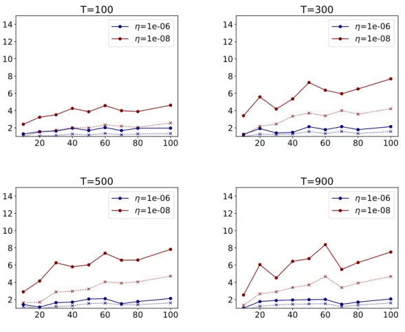
In Figure 1, we plot the obtained speed-up for different configurations:
• the final time T varies from 100 to 900,
• the final target accuracy isη= 10−6 orη = 10−8,
1
20
40
60
80
100
2
4
6
8
10
12
14
T=100
=1e-06
=1e-08
20
40
60
80
100
2
4
6
8
10
12
14
T=300
=1e-06
=1e-08
20
40
60
80
100
2
4
6
8
10
12
14
T=500
=1e-06
=1e-08
20
40
60
80
100
2
4
6
8
10
12
14
T=900
=1e-06
=1e-08
Figure 1: Speed-up as a function of the number of processors N. Dashed lines: classical parareal. Continuous lines: Adaptive parareal.
• the number of processorsN varies from 10 to 100.
As anticipated in section 3, the speed-up of the adaptive parareal is always superior to the one of the classical parareal. We observe that the gain is marginal for a moderate accuracy (η = 10−6) but it is about 2.5 times larger for η = 10−8. Note that sometimes the speed-up does not increase monotonically as the number of processors N increases. Also, the speed-up generally increases withN but the increase is rather moderate. We believe that this behavior could be improved with a rigorous a posteriori error estimator.
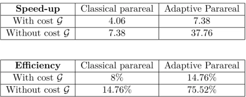
The values significantly differ from the range of full scalability and we next explain why this is mainly due to the cost of the coarse solver. Since the problem is stiff and we consider relatively long time intervals, it has been necessary to use a sufficiently accurate coarse solver. This explains our choice of an explicit Runge-Kutta scheme of order 5. To illustrate the impact of its cost, let us fix T = 500, η = 10−8 and N = 50 (other parameters would yield similar conclusions). We compare the speed-up and efficiency when we count or do not count the cost of the coarse solver on Table 1. Obviously, when we do not count the cost of the coarse solver, the performance of both algorithms improves but it is particularly increased in the case of the adaptive version. If the cost of G was negligible, it would deliver a very satisfactory efficiency of 75.52%. This is five times larger than what the classical parareal would yield. This analysis illustrates that the major obstacle to achieve competitive scalabilities is no longer the cost of the fine solver like in the classical version, but the cost of the coarse propagator.
Speed-up Classical parareal Adaptive Parareal
With costG 4.06 7.38
Without cost G 7.38 37.76
Efficiency Classical parareal Adaptive Parareal
With costG 8% 14.76%
Without cost G 14.76% 75.52%
Table 1: Impact of the cost of the coarse solver. Speed-up and efficiency with N= 50.
We fixT = 10,η = 10−8andN = 10 and plot in Figure 2 the convergence history of the parareal solution in terms of:
• the errors of the fine solver at every fine time-step
• the maximum error of the parareal solution at the macro-intervals max
N ku(TN)−y N k k
Note that the maximum error in the adaptive scheme steadily decreases to the desired accuracy whereas the error in the classical scheme degrades at iteration k= 1 before converging. This type of behavior has been observed for all other configurations and we conjecture that an important difference in accuracy between the coarse and the fine solver at early stages of the algorithm may be the cause. Finally, an inspection of the error of the fine solver shows that the adaptive algorithm succeeds to reduce the error at every time t in a much more uniform way than the classical algorithm.
5
Conclusions and perspectives
The new adaptive formulation of the parareal algorithm opens the door to improve significantly the parallel efficiency of the method provided that the cost of the coarse solver is moderate. The increasing target tolerances which have to be met at each step allows to use online stopping criteria involvinga posterioriestimators. The developed methodology remains theoretical since we have not quantified the impact of communication delays between processors nor potential memory issues (note however that the load balancing is devised with the purpose of equilibrating tasks and memory). In the framework of the ANR project “Ciné-Para (ANR-15-CE23-0019)”, we are working on these issues that are of a different level of theory and involve different collaborators. This will be the topic of another paper. In addition to this, several extensions based on the current findings are subject of ongoing works, in particular, the coupling of the adaptive parareal with adaptive space-time schemes and the coupling of parareal with internal iterative solvers like in the discussion of section A.3 of the appendix.
Acknowledgment
0.0 2.5 5.0 7.5 10.0 12.5 15.0 17.5 20.0 1012 1010 108 106 104 102 100 k=0 k=1 k=2 k=3 k=4 k=5 k=6 0 1 2 3 4 5 6 108 106 104 102 100 0 5 10 15 20 10-14 10-13 10-12 10-11 10-10 10-9 10-8 10-7 10-6 10-5 10-4 10-3 10-2 10-1 100 k=0 k=1 k=2 k=3 k=4 k=5 k=6 0 1 2 3 4 5 6 10-10 10-9 10-8 10-7 10-6 10-5 10-4 10-3 10-2 10-1
Figure 2: Convergence history of the errors. Top: classical parareal. Bottom: adaptive parareal. Left: Errors fort∈[0,10]. Right: maximum error at each iterationk.
A
Enriching the input information with previous iterations
Usually, solvers to realize [E(TN,∆T, ykN), ζkN] are built using onlyINk ={TN,∆T, yNk }as input
information. We account for this idea with the notation
S(TN,∆T, yNk)−−−−−−−→ (INk,cost
N k)
[E(TN,∆T, yNk);ζkN],
and the numerical cost, denoted costNk, increase as ζkN is tightened. In this section, we discuss how to enhance the gain in efficiency of the adaptive algorithm by discussing ways to increase the accuracy of the solver [E(TN,∆T, ykN), ζkN] across the iterations while maintaining the cost
to realize it as independent as possible fromζkN,N, andk. For this, one possibility is to enrich
INk with data produced during the previous parareal iterations (although it would of course be
at the cost of increasing the storage requirements).
Let PNk denote the intermediate information that has been produced at iteration k be-tween [TN, TN+1] and by Pk := ∪
N−1
N=0PNk all the information produced at step k. Using
eINk ={INk,PkN−1, . . . ,P0k,Pk−1, . . . ,P0}, as input information, the idea is to see whether it could be possible to find a solver S such that
S(TN,∆T, ykN)−−−−−−→ (eINk,cost)
[E(TN,∆T, yNk);ζkN] (19)
with a constant and small complexity cost. Note that using the enriched set of informa-tion eINk means that we want to learn from the previous approximations of u(TN+1) given by
[E(TN,∆T, yNp ), ζpN], 0 ≤ p ≤ k−1, to start the current algorithm closer to u(TN+1). After
each parareal iteration, we thus improve the accuracy, without increasing the work for solving because we start from a better input, accumulated from the previous parareal iterations.
In the rest of this section, we describe three relevant scenarios where we can approximate
E(TN,∆T, ykN) by trying to build a scheme in the spirit of (19). The first two examples have
already been presented in the literature and concern the coupling of parareal with spatial domain decomposition (section A.1) and with iterative high-order time integration schemes (section A.2). In these two cases, there is to date no complete convergence analysis since it remains to show that i) E(TN,∆T, yNk) is approximated with accuracy ζk and ii) the costof the solver is
really constant through the parareal steps. In addition to these two applications, we mention a third scenario where the convergence analysis can be fully proven. It concerns the solution of time-dependent problems involving internal iterative schemes at every time step. This idea was first analyzed in [27] in a restricted setting. In section A.3, we give the main setting and defer the analysis for a forthcoming paper.
A.1 Parareal coupled with spatial domain decomposition
Here, we consider a solverS =DDMwhich involves spatial domain decomposition over [TN, TN+1]
[16, 1]. We assume that DDM involves a time discretization with a small time step δt < ∆T. Let n be the number of time steps on each interval [TN, TN+1] so that we have the relations
∆T =nδtandT =N∆T =N nδtand the total number of time steps in [0, T] isn:=N n. The domain decomposition iterations act on a partition Ω =∪L
l=1Ωl of the domain. For 0≤n≤n,
we denote by uN,n,jk the solution produced by DDM at time t = TN +nδt after j ≥ 0 domain
decomposition iterations. The notation J∗ will denote the last iteration (fixed according to some stopping criterion). At j = 0, these iterations need to be initialized at the interfaces ∂Ωl, 1 ≤ l ≤ L. The idea explored in, e.g., [16, 1], is to take the values uN,n,Jk−1 ∗|∂Ωl at these interfaces as a starting guess for 0≤n≤n so that
e
INk ={INk,{u N,n,J∗
k−1 |∂Ωl,0≤n≤n}}.
From [16, 1], there is numerical evidence that the computations of DDM(TN,∆T, yNk) usingeINk yield [E(TN,∆T, yNk);ζkN] after a reduced number of iterations J∗ which is independent of k.
Thuscostwould be kept constant and
uN,n,Jk ∗ =DDM(TN,∆T, ykN)−−−−−−→ (eINk,cost)
[E(TN,∆T, yNk);ζkN],
where the above “cost” is much small than the cost of the fine solver.
A.2 Parareal coupled with iterative high-order time integration schemes
Spectral Deferred Correction (SDC, [10]) is an iterative time integration scheme. Starting from an initial guess ofu(t) at discrete points, the method adds successive corrections to this guess. The corrections are found by solving an associated evolution equation. Under certain conditions, the correction at every step increases by one the accuracy order of the time discretization.
We carry here a simplified discussion on how to build [E(TN,∆T, ykN);ζkN] when S = SDC
and connect it to the so-called Parallel Full Approximation Scheme in Space-Time (PFASST, [24, 11]). For a given time interval [TN, TN+1], let us consider its n+ 1 associated
Gauss-Lobatto points{tN,n}nn=0 and quadrature weights{ωn}nn=0. The Gauss-Lobatto points are such
iterationkafterj≥0 SDC iterations. Assuming that one uses an implicit time-stepping scheme to solve the corrector equations involved in this method,uN,nk +1,j is given by
uN,nk +1,j=ukN,n,j+ (tN,n+1−tN,n) A(tN,n+1, uN,nk +1,j)− A(tN,n+1, uN,nk +1,j−1) + n X m=0 ωmA(tN,m, uN,m,jk −1), 1≤j, 0≤n≤n−1, uN,k 0,j=yNk uN,n,k 0 given for 0≤n≤n.
To speed-up computations, one of the key elements is the choice of the starting guessesuN,n,k 0, 0≤
n≤n. Without entering into very specific details, the PFASST algorithm is a particular instan-tiation of the above scheme whenJ∗ = 1 anduN,n,k 0 uses information produced at the previous parareal iterationk−1. Therefore, PFASST falls into the present framework in the sense that it produces
uN,n,k 1 =SDC(TN,∆T, ykN)
with
eINk ={TN,∆T, ykN,Pk−1} and it is expected thatuN,n,k 1 = [E(TN,∆T, yNk );ζkN].
An additional component of PFASST is that the algorithm also tries to improve the accuracy of the coarse solverG using SDC iterations built witheIkN. This has not been taken into account in our adaptive parareal algorithm (11).
A.3 Coupling with internal iterative schemes
Any implicit discretization of problem (1) leads to discrete linear or nonlinear systems of equa-tions which are often solved with iterative schemes. When they are involved as internal iteraequa-tions within the parareal algorithm, one could try to speed them up by building good initial guesses based on information from previous parareal iterations. We illustrate this idea in the simple case where:
• A(t,·) is a linear differential operator in Ucomplemented with suitable boundary
condi-tions,
• we use an implicit Euler scheme for the time discretization.
A sequential solution of problem (1) with the implicit Euler scheme goes as follows. At each time tN,n =TN +nδt, the solution u(tN,n) is approximated by the functionuN,n∈U which is
itself the solution to
B(uN,n) =gN,n, wheregN,n=uN,n−1+δtf(tN,n) and
B(v) :=v+δtA(tN,n, v), ∀v ∈U.
Note that B depends on time but our notation does not account for it in order not to overload the notations.
After discretization of U, the problem classically reduces to solving a linear system of the form
for the unknown ¯uN,n in some discrete subspace S of U. Usually, the above system is solved either by means of a conjugate gradient method or by a Richardson iteration of the form
( ¯
uN,n,j = (Id+ωPB)¯uN,n,j−1+ωP¯b, j≥1 ¯
uN,n,0∈S given.
Here,ω is a suitably chosen relaxation parameter and Pcan be seen as a pre-conditioner. The internal iterationsjare stopped whenever a certain criterion is met (it could be an a posteriori estimator) and we denote by JN,n their final number. Obviously, JN,n depends on the starting
guess for which a usual choice is to take the solution at the previous time, that is ¯
uN,n,0= ¯uN,n−1,JN,n−1.
In order to achieve our goal, i.e. maintaning a low cost while increasing the accuracy at each parareal step, we can now reuse information from previous parareal iterations for the starting guess. In [27], two options are explored. The first is
¯ ukN,n,0 = ¯ukN,n−1,JN,n−1,k, ifk= 0 ¯ ukN,n,0 = ¯uN,n,Jk−1 N,n,k−1, ifk≥1, and the second, less natural choice,
¯ uN,n,k 0 = ¯uN,n−1,JN,n−1,k k , ifk= 0 ¯ uN,n,k 0 = ¯uN,n,JN,n,k−1 k−1 + ¯u N,n−1,JN,n,k k −u¯ N,n−1,JN,n−1,k−1 k−1 , ifk≥1.
In the first case, we take over the internal iterations at the point where they were stopped in the previous parareal iteration k−1. In addition to this, in the second case, the term uN,n−1,JN,n,k
k −u
N,n−1,JN,n−1,k−1
k−1 tries to better take the dynamics of the process into account.
Note that the use of solutions that have been produced in the previous parareal iterations is at the expense of additional memory requirements. It might also be at the cost of a certain increase in the complexity locally at certain times. However, [27] shows in a restricted setting that these starting guesses (in particular the second) have interesting potential to enhance the speed-up of the parareal algorithm. A general theory on this aspect will be presented in a forthcoming work.
References
[1] S. Aouadi, D. Q. Bui, R. Guetat, and Y. Maday,Convergence analysis of the coupled
parareal-schwarz waveform relaxation method, 2019. In preparation.
[2] L. Baffico, S. Bernard, Y. Maday, G. Turinici, and G. Zérah, Parallel-in-time
molecular-dynamics simulations, Physical Review E, 66 (2002), p. 057701.
[3] G. Bal and Y. Maday,A “parareal" time discretization for non-linear PDE’s with
appli-cation to the pricing of an American put, Recent developments in domain decomposition
methods, 23 (2002), pp. 189–202.
[4] G. Bal and Q. Wu, Symplectic parareal, in Domain decomposition methods in science and engineering XVII, Springer, 2008, pp. 401–408.
[5] Bal, G., Parallelization in time of (stochastic) ordinary differential equations, 2003. Preprint, http://www.columbia.edu/ gb2030/PAPERS/paralleltime.pdf.
[6] K. Carlberg, L. Brencher, B. Haasdonk, and A. Barth, Data-driven time
paral-lelism via forecasting, SIAM Journal on Scientific Computing, 41 (2019), pp. B466–B496.
[7] X. Dai, C. Le Bris, F. Legoll, and Y. Maday, Symmetric parareal algorithms for
hamiltonian systems, ESAIM: Mathematical Modelling and Numerical Analysis, 47 (2013),
pp. 717–742.
[8] X. Dai and Y. Maday,Stable parareal in time method for first- and second-order
hyper-bolic systems, SIAM J. Sci. Comput., 35 (2013), pp. A52–A78.
[9] J. R. Dormand and P. J. Prince,A family of embedded runge-kutta formulae, Journal of computational and applied mathematics, 6 (1980), pp. 19–26.
[10] A. Dutt, L. Greengard, and V. Rokhlin, Spectral deferred correction methods for
ordinary differential equations, BIT Numerical Mathematics, 40 (2000), pp. 241–266.
[11] M. Emmett and M. Minion,Toward an efficient parallel in time method for partial
dif-ferential equations, Communications in Applied Mathematics and Computational Science,
7 (2012), pp. 105–132.
[12] C. Farhat and M. Chandesris,Time-decomposed parallel time-integrators: theory and
feasibility studies for fluid, structure, and fluid–structure applications, International Journal
for Numerical Methods in Engineering, 58 (2003), pp. 1397–1434.
[13] M. Gaja and O. Gorynina,Parallel in time algorithms for nonlinear iterative methods, 2018. To appear in ESAIM Proceedings of CEMRACS 2016 – Numerical Challenges in Parallel Scientific Computing.
[14] M. J. Gander,50 years of time parallel time integration, in Householder Symposium XIX June 8-13, Spa Belgium, 2015, p. 81.
[15] M. J. Gander and E. Hairer, Nonlinear convergence analysis for the parareal
algo-rithm, in Domain Decomposition Methods in Science and Engineering XVII, Springer,
2008, pp. 45–56.
[16] R. Guetat,Méthode de parallélisation en temps: Application aux méthodes de
décompo-sition de domaine, PhD thesis, Paris VI, 2012.
[17] E. Hairer and G. Wanner, Solving Ordinary Differential Equations II. Stiff and
Differential-Algebraic Problems, vol. 14, 01 1996.
[18] E. Hairer and G. Wanner,Stiff differential equations solved by radau methods, Journal of Computational and Applied Mathematics, 111 (1999), pp. 93 – 111.
[19] J. Lions, Y. Maday, and G. Turinici, Résolution d’EDP par un schéma en temps
pararéel, C. R. Acad. Sci. Paris, (2001). t. 332, Série I, p. 661-668.
[20] Y. Maday, M. Ronsquist, E., and G. Staff,The parareal in time algorithm: Basics,
stability analysis and more, in Staff PhD Thesis, see below (2006), pp. 653–663.
[21] Y. Maday, J. Salomon, and G. Turinici, Monotonic parareal control for quantum
systems, SIAM Journal on Numerical Analysis, 45 (2007), pp. 2468–2482.
[22] Y. Maday and G. Turinici,The Parareal in Time Iterative Solver: a Further Direction
to Parallel Implementation, in Domain Decomposition Methods in Science and Engineering,
[23] M. Minion, A hybrid parareal spectral deferred corrections method, Comm. App. Math. and Comp. Sci., 5 (2010).
[24] M. Minion, A hybrid parareal spectral deferred corrections method, Communications in Applied Mathematics and Computational Science, 5 (2011), pp. 265–301.
[25] M. L. Minion, R. Speck, M. Bolten, M. Emmett, and D. Ruprecht,
Interweav-ing PFASST and parallel multigrid, SIAM Journal on Scientific Computing, 37 (2015),
pp. S244–S263.
[26] M. L. Minion, A. Williams, T. E. Simos, G. Psihoyios, and C. Tsitouras,Parareal
and spectral deferred corrections, in AIP Conference Proceedings, vol. 1048, 2008, p. 388.
[27] O. Mula, Some contributions towards the parallel simulation of time dependent neutron
transport and the integration of observed data in real time, PhD thesis, Paris VI, 2014.
[28] J. Nievergelt,Parallel methods for integrating ordinary differential equations, Commun. ACM, 7 (1964), pp. 731–733.
[29] A. Quarteroni and A. Valli, Domain decomposition methods for partial differential
equations, Von Karman institute for fluid dynamics, 1996.
[30] A. Toselli and O. Widlund, Domain decomposition methods: algorithms and theory, vol. 3, Springer, 2005.