Gaussian Multiresolution Models: Exploiting Sparse
Markov and Covariance Structure
Myung Jin Choi
, Student Member, IEEE
, Venkat Chandrasekaran
, Student Member, IEEE
, and
Alan S. Willsky
, Fellow, IEEE
Abstract—In this paper, we consider the problem of learning Gaussian multiresolution (MR) models in which data are only available at the finest scale, and the coarser, hidden variables serve to capture long-distance dependencies. Tree-structured MR models have limited modeling capabilities, as variables at one scale are forced to be uncorrelated with each other conditioned on other scales. We propose a new class of Gaussian MR models in which variables at each scale havesparse conditional covariance structure conditioned on other scales. Our goal is to learn a tree-structured graphical model connecting variables across scales (which trans-lates into sparsity in inverse covariance), while at the same time learning sparse structure for the conditional covariance (not its inverse) within each scale conditioned on other scales. This model leads to an efficient, new inference algorithm that is similar to multipole methods in computational physics. We demonstrate the modeling and inference advantages of our approach over methods that use MR tree models and single-scale approximation methods that do not use hidden variables.
Index Terms—Gauss–Markov random fields, graphical models, hidden variables, multipole methods, multiresolution (MR) models.
I. INTRODUCTION
M
ULTIRESOLUTION (MR) methods have been widely used in large-scale signal processing applications due to their rich modeling power as well as computational efficiency [34]. Estimation algorithms based on MR representations are efficient since they perform global computations only at coarser scales in which the number of variables is significantly smaller than at finer scales. In addition, MR models provide compact representations for long-range statistical dependencies among far-apart variables by capturing such behavior at coarser resolu-tions. One of the most common settings [3], [7], [8], [11], [19], [23], [28], [34] for representing MR models is that ofgraphical models, in which the nodes of the graph index random variables Manuscript received April 24, 2009; accepted September 22, 2009. First pub-lished November 06, 2009; current version pubpub-lished February 10, 2010. This work was supported in part by AFOSR under Grant FA9550-08-1-1080, in part by MURI under AFOSR Grant FA9550-06-1-0324, and in part by Shell Interna-tional Exploration and Production, Inc. The work of M. J. Choi was supported in part by a Samsung Scholarship. A preliminary version of this work appeared in the Proceedings of the 26th Annual International Conference on Machine Learning (ICML 2009), Montreal, QC, Canada. The associate editor coordi-nating the review of this manuscript and approving it for publication was Dr. Mark J. Coates.The authors are with the Department of Electrical Engineering and Computer Science, Laboratory for Information and Decision Systems, Massachusetts In-stitute of Technology, Cambridge, MA 02139 USA (e-mail: myungjin@mit. edu; [email protected]; [email protected]).
Color versions of one or more of the figures in this paper are available online at http://ieeexplore.ieee.org.
Digital Object Identifier 10.1109/TSP.2009.2036042
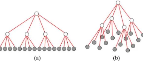
Fig. 1. Examples of MR tree models (a) for a 1-D process and (b) for a 2-D process. Shaded nodes represent original variables at the finest scale and white nodes represent hidden variables at coarser scales.
and the edges encode conditional independence structure among the variables. Graphical models in which edges are undirected are also called Markov random fields (MRFs).
In many applied fields including communication [13], speech and image processing [32], and bioinformatics [27], statistical models have been represented with sparse graphical model structures in which each node in the graph is connected to only a few other nodes. For Gaussian phenomena, in which the vari-ables being represented are jointly Gaussian, this corresponds to sparsity in the inverse covariance matrix. There are a variety of attractions of such sparse models, including parsimonious parameterization (with obvious advantages for learning such models and avoiding overfitting) and the potential for efficient inference algorithms (e.g., for computing posterior distributions given measurements or for parameter estimation).
The potential advantages of sparsity for efficient inference, however, depend very much on the structure of the resulting graph, with the greatest advantage for tree-structured graphs, i.e., graphs without cycles. Indeed, this advantage provided one of the major motivations for the substantial literature and appli-cation [10], [14], [22], [34] of models on MR trees (such as in Fig. 1) in which each level represents the phenomenon of in-terest at a corresponding scale or resolution. The coarser scales in these models are usually introduced solely or primarily1as hidden variables. That is, it is the finest scale of such a model that represents the phenomenon of interest, and coarser scales are introduced to capture long-range correlations in a manner that is graphically far more parsimonious than could be cap-tured solely within a single, finest scale model. Indeed, a sparse single-scale graphical model is often poor at capturing long-range correlations, and even if it does, may result in the model being ill-conditioned.
A significant and well-known limitation of such MR tree models, however, is the set of statistical artifacts they can
1In some contexts, some of the variables at coarser scales represent nonlocal
functionals of the finest scale phenomenon that are either measured or are to be estimated.
introduce. In an MR tree model, variables at one scale are
conditionally independent when conditioned on neighboring scales, a direct consequence of the fact that nodes are connected to each other only through nodes at other scales. Thus, the corre-lation structure between variables at the finest scale can depend dramatically on exactly how the MR tree is arranged over these finest scale nodes. In particular, finest scale nodes that are the same “distance” from each other as measured solely within that finest scale can have very different distances along the MR tree due to the different lengths of fine-to-coarse-to-fine paths that connect them. While in some applications such fine-scale arti-facts may have no significant effect on the particular estimation task of interest, there are many situations in which these arti-facts are unacceptable. A variety of methods [3], [7], [8], [11], [19], [23], [28] have been proposed to overcome this limitation of tree models. These methods involve including additional edges—either interscale or within the same scale—to the MR tree model and considering an overall sparse MR graphical model.
In this work, we propose a different approach to address the limitation of MR tree models—one that has considerable intu-itive appeal. Note that the role of coarser scales in an MR model is to capture most of the correlations among the finer scale vari-ables through coarser scales. Then, should not theresidual cor-relations at each scale that need to be captured be approximately
local? In other words, conditioned on variables at other scales, the residual correlation of any node should be concentrated on a small number of neighboring nodes within the same scale. This suggests that instead of assuming that the conditional sta-tistics at each scale (conditioned on the neighboring scales) have sparse graphical structure (i.e., sparse inverse covariance) as in the previous methods, we need to look for models in which the
conditionalstatistics havesparse covariance structure. MR models with the type of structure described above—tree-structure between scales and then sparse conditional covariance structure within each scale—have a special inverse covariance structure. As we describe later in the paper, the inverse covari-ance matrix of our MR model (denoted ) can be represented as a sum of the inverse covariance matrix of an MR tree (denoted ) and inverse of a conditional covariance matrix within each
scale (denoted ), i.e., where both
and are sparse matrices. This structure leads to efficient estimation algorithms that are different in a fundamental way from standard graphical model estimation algorithms which exploit sparse graph structure. Indeed, as we describe in this paper, sparse in-scale conditional correlation structure gener-ally corresponds to adensegraphical model within each scale, so that standard graphical model inference algorithms are not useful. However, estimation for phenomena that are only locally correlated requires local computations—essentially a general-ization of finite impulse response (FIR) filtering within each scale—corresponding to multiplication involving the sparse conditional covariance matrix. Our approach can be viewed as a statistical counterpart to so-calledmultipole methods[20] for the rapid solution of elliptic partial differential equations (in particular those corresponding to evaluating electric fields given charge distributions); we use the sparse tree structure ofpartof the overall statistical structure, namely, thatbetweenscales, to
propagate information from scale-to-scale (exploiting sparsity in ), and then perform local FIR-like residual filteringwithin
each scale (exploiting sparsity in ).
In addition to developing efficient algorithms for inference given our MR model, we develop in detail methods forlearning
such models given data at the finest scale (or more precisely an empirical marginal covariance structure at the finest scale). Our modeling procedure proceeds as follows: given a collec-tion of variables and a desired covariance among these ables, we construct an MR model by introducing hidden vari-ables at coarser resolutions. Then, we optimize the structure of each scale in the MR model to approximate the given statis-tics with asparse conditional covariance structurewithin each scale. This step can be formulated as a convex optimization problem involving the log-determinant of the conditional co-variance matrix.
The rest of the paper is organized as follows. In the next sec-tion, we provide some background on graphical models and a sparse matrix approximation method using log-determinant maximization. In Section III, the desired structure of our MR model—sparse interscale graphical structure and sparse in-scale conditional covariance structure—is specified in detail. The spe-cial-purpose inference algorithm that exploits sparsity in both Markov and covariance structure is described in Section IV, while in Section V, we show how the log-det maximization problem can be used to learn our MR models. In Section VI, we illustrate the advantages of our framework in three mod-eling problems: dependencies in monthly stock returns, frac-tional Brownian motion [30], and a 2-D field with polynomially decaying correlations. We provide experimental evidence that our MR model captures long-range correlations well without blocky artifacts, while using many fewer parameters than single-scale approximations. We also demonstrate that our MR ap-proach provides improved inference performance. Section VII concludes this paper, and in Appendixes I–III, we provide algo-rithmic details for our learning method.
II. PRELIMINARIES A. Gaussian Graphical Models
Let be a graph with a set of nodes and (pair-wise) edges . Two nodes and are said to be neighborsif there is an edge between them. A subset of nodes is said toseparatesubsets if every path in between any node in and any node in passes through a node in . A graphical model is a collection of random variables indexed by nodes of the graph: each node is associated with a random
variable ,2and for any . A
proba-bility distribution is said to beMarkovwith respect to a graph if for any subsets that are separated by some and are independent conditioned on . Specifically, if an edge is not present between two random variables, it indicates that the two variables are independent conditioned on all other variables in the graph.
2For simplicity, we assume thatx is a scalar variable, but any of the analysis
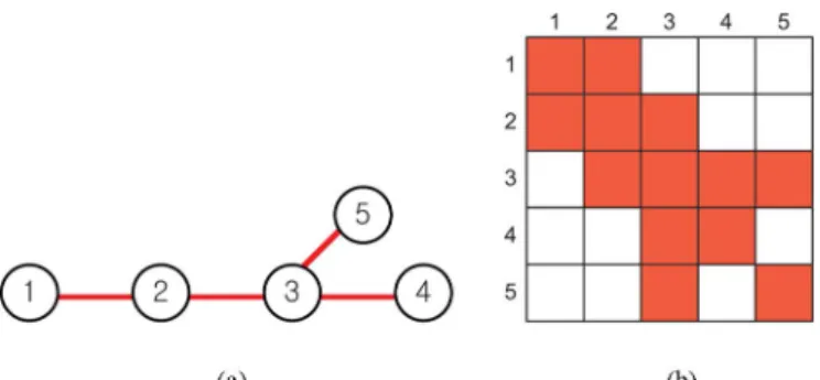
Fig. 2. (a) Sparse graphical model. (b) Sparsity pattern of the corresponding information matrix.
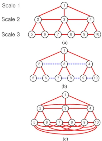
Fig. 3. Conjugate graph. (a) Sparsity pattern of a covariance matrix. (b) Corre-sponding graphical model. (c) Conjugate graph encoding the sparsity structure of the covariance matrix in (a).
Let be a jointly Gaussian random vector with a mean vector and a positive–definite covariance matrix . If the variables are Markov with respect to a graph , the inverse of the covariance matrix (also called the in-formation, or precision, or concentration matrix) is sparse with respect to [26]. That is, if and only if . We use to denote a Gaussian distribution with an in-formation matrix and a potential vector ; the
distri-bution has the form . Fig. 2(a)
shows one example of a sparse graph, and the sparsity pattern of the corresponding information matrix is shown in Fig. 2(b). The graph structure implies that is uncorrelated with con-ditionedon . Note that this does not indicate that is uncor-related with . In fact, the covariance matrix (the inverse of the information matrix) will, in general, be a full matrix.
For any subset , let be its
complement. Then, the conditional distribution is Markov with respect to the induced subgraph of with nodes
and edges . The
corre-sponding information matrix of the conditional model is the sub-matrixof with rows and columns corresponding to elements in . For example, in Fig. 2, is a chain model connecting variables through , and the information matrix of this conditional distribution is the submatrix , which is a tri-diagonal matrix.
B. Conjugate Graphs
While Gaussian graphical models provide a compact repre-sentation for distributions with a sparse information matrix, in general, a sparse graphical model cannot represent distributions with a sparsecovariancematrix. Consider a distribution with the sparsity pattern of thecovariance matrixgiven as in Fig. 3(a). Its information matrix will, in general, be a full matrix, and the corresponding graphical model will be fully connected as shown in Fig. 3(b). Therefore, we introduceconjugate graphsto illus-trate the sparsity structure of a covariance matrix. Specifically,
in the conjugate graph, when two nodes are not connected with a
conjugateedge, they areuncorrelatedwith each other.3We use
solid lines to display graphical model edges, and dotted lines to represent conjugate edges. Fig. 3(c) shows the corresponding conjugate graph for a distribution with covariance structure as in Fig. 3(a). From the conjugate edge structure, we can identify that is uncorrelated with , and .
The term conjugate graph is motivated by the notion of con-jugate processes [25]—two random processes that have covari-ances that are inverses of one another.4Our concept of a
con-jugate graph that represents marginal independence structure is also called acovariance graphor abi-directed graph[12], [16], [24].
C. Log-Determinant Maximization
In this section, we introduce the log-determinant maximiza-tion problem to obtain a positive–definite matrix that approxi-mates a given target matrix and has a sparse inverse. This tech-nique will be used in Section V to learn a sparse graphical model approximation or a sparse covariance matrix approxima-tion. Suppose that we are given a target matrix , and we wish to learn an approximation that is positive–definite and has a sparse inverse. Thresholding the elements of can be in-effective as the resulting matrix may not be positive–definite. One alternative is to solve the following convex optimization problem of maximizing the log-determinant of subject to el-ementwise constraints with respect to the target matrix:
(1) where is a nonnegative regularization parameter and is a convex distance function. In Section V, we use the abso-lute difference between the two values as the distance
func-tion: . Note that this optimization
problem is convex in . In the following proposition, we show that when is large enough, a set of elements of the inverse of
are forced to be zero.
Proposition 1: Assume that for all and that the feasible set of (1) is nonempty. Then, for each such that the inequality constraint is not tight [i.e., ], the corresponding element of is zero [i.e., ].
Proof: From the Karush–Kuhn–Tucker (KKT) conditions [4], there exists for all such that the following equations are satisfied:
where is a matrix with its elements
. The first equation is also called the complementary slackness condition. The second equation is
obtained using . For all such
that , we get from the first equation.
Since from the second equation, for each that the equality constraint is not tight, .
3Since we consider jointly Gaussian variables, uncorrelated variables are
in-dependent.
This optimization problem is commonly used in Gaussian modeling to learn a sparse graphical model approximation given the target covariance [1] as we describe in Section V-A. We also use the same framework to learn asparse covariance matrix ap-proximationgiven the target information matrix as described in Section V-B.
III. MULTIRESOLUTIONMODELSWITHSPARSEIN-SCALE CONDITIONALCOVARIANCE
We propose a class of MR models with tree-structured con-nections between different scales and sparse conditional covari-ance structure at each scale. Specifically, within each scale, a variable is correlated with only a few other variables in the same scaleconditionedon variables at scales above and below. We il-lustrate the sparsity of thein-scale conditional covarianceusing the conjugate graph. Thus, our model has a sparse graphical model for interscale structure and a sparse conjugate graph for in-scale structure. In the rest of the paper, we refer to such an MR model as a sparse in-scale conditional covariance multires-olution (SIM) model.
We would like to emphasize the difference between the con-cept of in-scale conditional covariance with the more com-monly used concepts ofmarginal covarianceandpairwise con-ditional covariance. Specifically, marginal covariance between two variables is the covariance without conditioning on any other variables. Pairwise conditional covariance refers to the conditional covariance between two variables when conditioned onall other variables, including the variables within the same scale. In-scale conditional covariance is the conditional covari-ance between two variables (in the same scale) when condi-tioned onvariables at other scales(or equivalently, variables at scales above and below, but not the variables at the same scale). As we illustrate subsequently in this section, the distinction between SIM models and the class of MR models with sparse pairwise conditional covariance structure is significant in terms of both covariance/information matrix structure and graphical model representation. The latter, which has been the subject of study in previous work of several authors, has sparse informa-tion matrix structure and, corresponding to this, sparse struc-ture as a graphical model, including within each scale. In con-trast, our SIM models have sparse graphical model structure be-tweenscales but generally havedense conditional information matriceswithin each scale. At first this might seem to be unde-sirable, but the key is that the conditionalcovariancematrices within each scalearesparse—something we display graphically using conjugate graphs. As we show in subsequent sections, this leads both to advantages in modeling power and efficient inference.
Fig. 4(b) shows an example of our SIM model. We denote the coarsest resolution asscale 1and increase the scale number as we go to finer scales. In the model illustrated in Fig. 4(b),
conditionedon scale 1 (variable ) and scale 3 (variables through ), isuncorrelatedwith . Note that this is dif-ferent from and being uncorrelated without conditioning on other scales (the marginal covariance is nonzero), and also different from the corresponding element in the information ma-trix being zero (the pairwise conditional covariance is nonzero). In fact, the corresponding graphical model representation of the
Fig. 4. Examples of MR models. (a) MR model with a sparse graphical struc-ture. (b) SIM model with sparse conjugate graph within each scale. (c) Graphical model corresponding to the model in (b).
model in Fig. 4(b) consists of a densely connected graphical structure within each scale as shown in Fig. 4(c).
In contrast, an MR model with a sparse graphical model struc-ture within each scale is shown in Fig. 4(a).5Such a model does
not enforce sparse covariance structure within each scale condi-tioned on other scales: condicondi-tioned on scales above and below, and are correlated unless we condition on the other vari-ables at the same scale (namely variable ). In Section VI, we demonstrate that SIM models lead to better modeling capabili-ties and faster inference than MR models with sparse graphical structure.
The SIM model, to our best knowledge, is the first approach to enforce sparse conditional covariance at each scale explicitly in MR modeling. A majority of the previous approaches to over-coming the limitations of tree models [7], [8], [11], [23], [28] focus on constructing an overall sparse graphical model struc-ture [as in Fig. 4(a)] to enable an efficient inference procedure. A different approach based on a directed hierarchy of densely con-nected graphical models is proposed in [32], but it does not have a sparse conjugate graph at each layer and requires mean-field approximations unlike our SIM model.
A. Desired Structure of the Information Matrix
A SIM model consists of a sparse interscale graphical model connecting different scales and a sparse in-scale conditional
co-5Throughout this paper, we use the term “sparse” loosely for coarser scales
with just a few nodes. For these coarse scales, we have a small enough number of variables so that computation is not a problem even if the structure is not sparse.
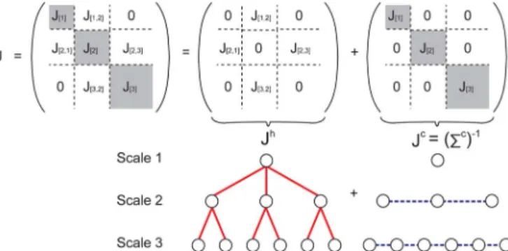
Fig. 5. Decomposition of a SIM model into a sparse hierarchical structure con-necting different scales and a sparse conjugate graph at each scale. Shaded ma-trices are dense and nonshaded mama-trices are sparse.
variance matrix at each scale. Here, we specify the desired spar-sity structure for each submatrix of the information matrix of a SIM model. First, we partition the information matrix of a SIM model by scale as shown in Fig. 5 (corresponding to a model with three scales). The submatrix of corresponds to the information matrix of theconditionaldistribution at scale conditioned on other scales (see Section II-A). As illustrated in Fig. 4(c), a SIM model has a densely connected graphical model within each scale, so in general is not a sparse ma-trix. The inverse of , however, is sparse since we have a sparse conditional covariance matrix within each scale. The sub-matrix is sparse with respect to the graphical model structure connecting scale and . We consider hierarchical models in which only successive neighboring scales are
con-nected. Hence, is a zero matrix if .
By the modeling assumption that the interscale graphical model connecting different scales is sparse, is a sparse matrix. In Fig. 5, shaded matrices are dense and non-shaded matrices are sparse.
The matrix can be decomposed as a sum of , corre-sponding to the hierarchical interscale tree structure, and , corresponding to the conditional in-scale structure. Let
. Since is a block-diagonal matrix, its inverse is also block-diagonal with each diagonal block equal to . Hence, is a sparse matrix, whereas is not sparse in gen-eral. Therefore, the information matrix of a SIM model can be decomposed as a sum of a sparse matrix and the inverse of a sparse block-diagonal matrix
(2) Each nonzero entry in corresponds to an interscale edge con-necting a pair of variables at different scales. The block diagonal matrix has nonzero entries corresponding toconjugateedges within each scale. One simple example is demonstrated in Fig. 5. In Section IV, we take advantage of sparsity inboth and for efficient inference.
IV. INFERENCEEXPLOITINGSPARSITY INMARKOV AND COVARIANCESTRUCTURE
Let be a collection of random variables with a prior distri-bution: . Suppose that we have a set of noisy measurements at a subset of the variables: where
is a selection matrix that only selects variables at which mea-surements are specified, and is a zero-mean Gaussian noise vector with covariance . The maximuma posteriori(MAP) estimate is equivalent to the mean of the posterior distribution (3)
where , and . The posterior
infor-mation matrix has the same sparsity structure as if we assume that the noise covariance matrix is diagonal. If corresponds to a tree-structured model, (3) can be solved with linear complexity. If the prior model is not a tree, solving this equation directly by matrix inversion requires computa-tions where is the number of variables. We review a class of iterative algorithms that solve linear systems using the idea of a
matrix splittingin Section IV-A. Based on the specific splitting of the information matrix of our SIM model as in (2), we pro-pose a new and efficient inference algorithm in Section IV-B.
A. Iterative Algorithms Based on a Matrix Splitting
As described above, computing the optimal estimates in Gaussian models is equivalent to solving a linear equation where is a posterior information matrix. Many iterative linear system solvers are based on the idea of a matrix splitting: . Let us rewrite the original equation as . Assuming that is invertible, we obtain the following iterative update equations:
(4) where is the value of at the previous iteration, and is the updated value at the current iteration. The matrix is called apreconditioner, and (4) corresponds to the precondi-tioned Richardson iterations [18]. If solving the equation
for a fixed vector is easy due to a special structure of , each iteration can be performed efficiently.6There are a variety
of ways in which splittings can be defined [15]. For example, Gauss–Jacobi iterations set the preconditioner as a diagonal matrix with diagonal elements of , and embedded tree (ET) algorithms [33] split the matrix so that has a tree structure.
B. Efficient Inference in SIM Models
We use the matrix splitting idea in developing an efficient in-ference method for our SIM model. Recall that the informa-tion matrix of the SIM model can be decomposed as in (2). Our goal is to solve the equation
where , and are all sparse matrices. We alternate be-tween two inference steps corresponding tointerscale compu-tation and in-scalecomputation in the MR model. Our inter-scale computation, called thetree inference stepexploits sparse Markov structure connecting different scales, while ourin-scale inference step exploits sparse in-scale conditional covariance structure within each scale.
1) Tree Inference: In the tree-inference step, we select the interscale tree structure as the preconditioner in (4) by setting
6We may use different preconditioners for each iteration, resulting in
, where is a diagonal matrix added to ensure that is positive–definite7
(5) With the right-hand side vector fixed, solving the above equa-tion is efficient since corresponds to a tree-structured graph-ical model.8On the right-hand side, can be evaluated easily
since is diagonal, but computing directly is not efficient because is a dense matrix. Instead, we eval-uate bysolving the matrix equation . The matrix (in-scale conditional covariance) is sparse and well-condi-tioned in general; hence the equation can be solved efficiently. In our experiments, we use just a few Gauss–Jacobi iterations (see Section IV-A) to compute .
2) In-scale Inference: In this step, we select the in-scale structure to perform computations within each scale by setting . Then, we obtain the following update equation:
(6) Evaluating the right-hand side only involves multiplications of a sparse matrix and a vector, so can be computed efficiently. Note that although we use a similar method of split-ting the information matrix and iteratively updasplit-ting as in the Richardson iteration (4), our algorithm is efficient due to a fun-damentally different reason. In the Richardson iteration (specif-ically, the ET algorithm) and in the tree-inference step, solving the matrix equation is efficient because it is equivalent to solving an inference problem on a tree model. In our in-scale infer-ence step, the preconditioner selected actually corresponds to a densely connected graphical model, but since it has a sparse conjugate graph, the update equation reduces to a sparse ma-trix multiplication. Thus, our in-scale inference step requires onlylocalcomputations, which is in the same spirit as multi-pole methods [20] or FIR filtering methods.
After each iteration, the algorithm checks whether the pro-cedure has converged by computing the relative residual error:
where is the norm
and . The term can be
evalu-ated efficiently even though is not a sparse matrix. Since
, the value of
com-puted from the tree-inference step can be used to evaluate the residual error as well, and since and are sparse matrices, the first two terms can be computed efficiently.
The concept of performing local in-scale computations can be found in algorithms that use multiple scales to solve partial dif-ferential equations, such as multipole methods [20] or multigrid methods [5]. The efficiency of these approaches comes from the assumption that after a solution is computed at coarser resolu-tions, onlylocalterms need to be modified at finer resolutions. However, these approaches do not have any statistical basis or interpretation. The models and methods presented in this paper
7In (4),Mneeds to be invertible, but(J +J )is singular since the diagonal
elements at coarser scales (without measurements) are zero. In our experiments, we useD = (diag(6 )) wherediag(6 )is a diagonal matrix with diagonal elements of6 .
8This step is efficient for a more general model as well in which the interscale
structure is sparse but not a tree.
are aimed at providing a precise statistical framework leading to inference algorithms with very solid advantages analogous to those of multipole and multigrid methods.
V. LEARNINGMR MODELSWITHSPARSEIN-SCALE CONDITIONALCOVARIANCE
In this section, we describe the procedure of learning a SIM model approximation to a given target covariance. As has been well-developed in the literature and reviewed in Section V-A, optimization of the log-determinant of a covariance matrix leads to sparse inverse covariances and hence sparse graphical models. In Section V-B, we turn the tables—optimizing the log-determinant of the inverse covariance to yield a sparse covariance. We learn SIM models with sparse hierarchical graphical structure and sparse in-scale conditional covariance structure by combining these two methods as described in Section V-C.
A. Sparse Graphical Model Approximation
Suppose that we are given a target covariance and wish to learn a sparse graphical model that best approximates the co-variance. The target covariance matrix may be specified exactly when the desired statistics of the random process are known, or may be the empirical covariance computed from samples. One possible solution for selecting a graphical model is to use the inverse of the target covariance matrix, . However, whether is exact or empirical, its inverse will, in general, be a full matrix, resulting in a fully connected graphical model. One may threshold each element of so that small values are forced to zero, but often, this results in an invalid covariance matrix that is not positive–definite.
Therefore, standard approaches in Gaussian graphical model selection [1], [17], [21] use the log-determinant problem in (1) to find an approximate covariance matrix
(7) From Proposition 1, the solution of the above problem has a sparse inverse, which is a sparse graphical model approxima-tion. The entropy of a Gaussian distribution is proportional to the log-determinant of its covariance matrix. Hence, this learning approach is also called maximum-entropy modeling [21].
It can be shown that the dual problem of (7) is given as follows [1]:
(8)
where , and
is the divergence between the two distributions. This problem minimizes the divergence between the approximate and the original distribu-tion with an penalty on the elements of to obtain a sparse graphical model approximation. Both the primal (7) and the dual (8) optimization problems are convex and can be solved efficiently using interior-point methods [21], block coordinate descent methods [1], or the so-called graphical lasso [17].
B. Sparse Covariance Approximation
We now consider the problem of approximating a target dis-tribution with a disdis-tribution that has a sparsecovariancematrix (as opposed to a sparse information matrix as in the previous section). That is, we wish to approximate a target Gaussian dis-tribution with information matrix by a distribution in which many pairs of the variables are uncorrelated. We again use the log-determinant problem in (1), but now in the information ma-trix domain
(9) The solution has a sparse inverse, leading to a sparse covari-ance approximation. Note the symmetry between (7) and (9). In a Gaussian model, thelog-partition function[7] is proportional to the negative of the log-determinant of the information ma-trix. Thus, the problem in (9) can be interpreted asminimizing the log-partition function.
In our MR modeling approach, we apply this sparse covari-ance approximation method to model distributions at each scale conditioned on other scales. Thus, the conditional distribution at each scale is modeled as a Gaussian distribution with a sparse covariance matrix.
C. Learning a SIM Model
In this section, we discuss a method to learn a SIM model to approximate a specified MR model that has some complex structure (e.g., without the local in-scale conditional covariance structure). When a target covariance (or graphical model) is specified only for the finest scale variables, we first need to construct a full MR model that serves as the target model for the SIM approximation algorithm; such an “exact” target MR model must have the property that the marginal covariance at the finest scale equals the specified covariance for the finest scale variables.
Appendix I describes in detail the algorithm that we use to produce a target MR information matrix if we are only pro-vided with a target covariance at the finest scale. The basic idea behind this approach is relatively simple. First, we use an EM algorithm to fit an MR tree model so that themarginal covari-ance at each finest scale node in this model matches those of the provided finest scale target covariance. As is well known, because of the tree structure of this MR model, there are often artifacts across finest scale tree boundaries, a manifestation of the fact that such a model does not generally match the joint statistics, i.e., the cross covariances, across different finest scale nodes. Thus, we must correct the statistics at each scale of our MR model in order to achieve this finest scale matching. There-fore, in our second step, we introduce correlations within each scale resulting in a full target whose finest scale marginal co-variance matches the originally given coco-variance. Referring to Fig. 5, what the first tree construction does is to build the tree-structured information matrix , capturing interscale connec-tions, as well as a first approximation to the diagonal of the in-scale conditional covariance . What the second step does is to fill in the remainder of the shaded blocks in and modify the diagonals in order to match the finest scale marginal
statis-tics. In so doing, this target covariance does not, in general, have sparse in-scale conditional covariance (i.e., is
not sparse), and the procedure we now describe (with many more details in Appendixes II and III) takes the target
and produces an approximation that has our desired SIM structure.
Suppose that the target MR model is specified in information form with information matrix . We can find a SIM model that approximates by solving the following optimization problem:
(10) where is the in-scale information matrix at scale and is the set of all possible interscale edges connecting successive neighboring scales. Note that except for the posi-tive–definiteness condition , the objective function as well as the constraints can be decomposed into an interscale component and in-scale components. If we only look at the terms involving the parameters at scale (i.e., elements of the matrix ), the above problem maximizes the log-deter-minant of the information matrix subject to elementwise constraints. Therefore, from the arguments in Section V-B, the log-det terms ensure that each has a sparse inverse, which leads to a sparse in-scale conditional covariance, and thus a sparse conjugate graph. The -norm on the interscale edges penalizes nonzero elements [performing the same role as in the second term of (8)] and thus encourages the interscale structure connecting different scales to be sparse. Often, the specified target information matrix of the MR model already has a sparse interscale graphical structure, such as an MR tree structure (see Appendix I, for example). In such a scenario, the
-norm can be dropped from the objective function.
The problem in (10) is convex and can be efficiently solved using general techniques for convex optimization [4], [29]. In Appendixes II and III, we provide a simplified version of the problem in (10) to further reduce the computational complexity in solving the optimization problem. This can be achieved by interleaving the procedure of constructing the target MR model and the optimization procedure at each scale to obtain a sparse conjugate graph structure scale-by-scale. The regularization pa-rameter in the constraints of (10) provides a tradeoff between sparsity of the in-scale conjugate graphs and data-fidelity (i.e., how close the approximation is to the target information ma-trix ). In practice, we allow two different regularization pa-rameters for each scale: one for all node constraints and one for all edge constraints. For our experimental results, we se-lected these regularization parameters using a heuristic method described in Appendix III.
VI. EXPERIMENTALRESULTS
Modeling of complex phenomena is typically done with an eye to at least two key objectives: 1) model accuracy; and 2) tractability of the resulting model in terms of its use for various statistical inference tasks.
In this section, we compare the performance of our SIM model to four other modeling approaches. First, we consider
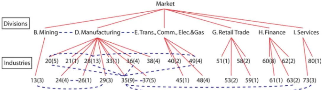
Fig. 6. Structure of the SIM model approximation for stock data. TABLE I
TOPFOURSTRONGESTCONJUGATEEDGES ATSCALE3OFFIG. 6
a single-scale approximate model where we learn a sparse graphical model using (7) without introducing hidden vari-ables. This is motivated by the fact that one of the dominant themes in statistical modeling is to encourage a sparse graphical model structure to approximate given statistics. Another widely used modeling method is a tree-structured MR model. Such tree models are the absolute winner in terms of computational tractability, but they are not nearly as good in terms of modeling accuracy. Third, we consider a sparse MR model in the form introduced in [7], which aims to overcome the limitations of the tree. Note that unlike a SIM model, a sparse MR model has a sparse information matrix butnotsparse in-scale conditional covariance. Finally, for each of our examples, we have the original model defined by the exact given statistics. They serve as target statistics for each approximate modeling method, but they do not have a sparse structure that makes inference computationally tractable in larger examples.
We measure the modeling accuracy of approximate models by computing the divergence between the exact distribution and the approximate distribution.9The tractability of each model can
be evaluated either by measuring computation time for a spe-cific inference task or by counting the number of parameters. An important point here is that all of the methods to which we compare, as well as our SIM model, are general-purpose mod-eling frameworks that are not tailored or tuned to any specific application.
A. Stock Returns
Our first experiment is modeling the dependency structure of monthly stock returns of 84 companies in the S&P 100 stock index.10 We use the hierarchy defined by the Standard Indus-9For multiscale models, we marginalize out coarser scale variables and use
the marginal covariance at the finest scale to compute this divergence.
10We disregard 16 companies that have been listed on S&P 100 only after
1990.
Fig. 7. Stock returns modeling example. Sparsity pattern of the information matrix of (a) the single-scale (122.48), and (b) the sparse MR approximation (28.34). (c) Sparsity pattern of the in-scale conditional covariance of the SIM approximation (16.36). All at the finest scale. We provide the divergence be-tween the approximate and the empirical distribution in the parenthesis. The tree approximation has divergence 38.22.
trial Classification (SIC) system,11which is widely used in
fi-nance, and compute the empirical covariance using the monthly returns from 1990 to 2007. Our MR models have four scales, representing the market, six divisions, 26 industries, and 84 in-dividual companies, respectively, at scales from the coarsest to the finest.
Fig. 6 shows the first three scales of the SIM model approx-imation. At scale 3, we show the SIC code for each industry (represented by two digits) and in the parenthesis denote the number of individual companies that belong to that industry (i.e., number of children). We show the finest scale of the SIM model using the sparsity pattern of thein-scale conditional co-variancein Fig. 7(c). Often, industries or companies that are closely related have a conjugate edge between them. For ex-ample, the strongest conjugate edge at scale 3 is the one between the oil and gas extraction industry (SIC code 13) and the petro-leum refining industry (SIC code 29). Table I shows four con-jugate edges at scale 3 in the order of their absolute magnitude (i.e., the top four strongest in-scale conditional covariance).
Fig. 7(a) shows the sparsity pattern of theinformation ma-trixof a single-scale approximation. Note that the corresponding graphical model has densely connected edges among companies
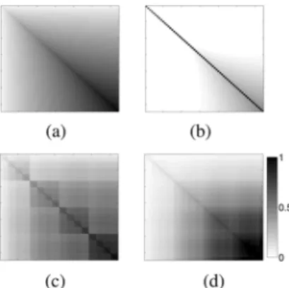
Fig. 8. Covariance approximation for fBm-64. (a) Original model. (b) Single-scale approximation. (c) Tree approximation. (d) SIM model.
that belong to the same industry, because there is no hidden vari-able to capture the correlations at a coarser resolution. Fig. 7(b) shows the information matrix at the finest scale of a sparse MR model approximation [8]. Although the graphical model is sparser than the single-scale approximation, some of the compa-nies still have densely connected edges. As shown in the caption of Fig. 7, the SIM model approximation provides the smallest divergence of all approximations.
B. Fractional Brownian Motion
We consider fractional Brownian motion (fBm) [30] with Hurst parameter defined on the time in-terval with the covariance function:
. Note that this is a nonstationary process. Fig. 8 shows the covariance realized by each model using 64 time samples. For the tree model and the SIM model, we only show the marginal covariance of the finest scale variables. Our SIM approximation in Fig. 8(d) is close to the original covariance in Fig. 8(a), while the single-scale ap-proximation in Fig. 8(b) fails to capture long-range correlations and the tree model covariance in Fig. 8(c) appears blocky.
A similar covariance realization without severe blocky arti-facts can also be obtained by the sparse MR model of [7]. How-ever, we observe that a SIM model can achieve a smaller di-vergence with respect to the true model with a smaller number of parameters than the counterpart sparse MR model. Fig. 9(a) shows the sparsity pattern of the conjugate graph (i.e., the con-ditional covariance) of the finest scale of the SIM model and Fig. 9(b) shows the sparsity pattern of the graphical model (i.e., the information matrix) of the finest scale of the sparse MR model. The SIM model has 134 conjugate edges at the finest scale and the sparse MR model has 209 edges. The divergence with respect to the true distribution is 1.62 for the SIM model and 2.40 for the sparse MR model. Moreover, note that the struc-ture of the conjugate graph in Fig. 9(a) is mostly local, but in the sparse MR model in Fig. 9(b), some nodes are connected to many other nodes. This suggests that the conditional covariance structure is a more natural representation for capturing in-scale statistics.
Fig. 10(a) displays a 256-point sample path using the exact statistics and Fig. 10(b) displays sparse and noisy observations of Fig. 10(a). Observations are only available on (over
Fig. 9. Sparsity pattern of (a) the in-scale conditional covariance of the finest scale of the SIM model and (b) the information matrix of the finest scale of the sparse MR model for the fBm-64 example.
Fig. 10. Estimation for fBm-256. (a) Sample-path using exact statistics. (b) Noisy and sparse observations of (a). Estimates using (c) single-scale ap-proximation, (d) tree model, and (e) SIM model are shown in the dashed–dotted lines. In each figure, the solid black line indicates the optimal estimate based on exact statistics, and the dashed gray lines show plus/minus one standard deviation error bars of the optimal estimate.
TABLE II FBM-256 APPROXIMATION
which the noise variance is 0.3) and (with noise vari-ance 0.5). Fig. 10(c)–(e) shows the estimates (in dashed–dotted line) based on the approximate single-scale model, the tree, and the SIM model, respectively, together with the optimal esti-mate based on the exact statistics (in solid black). The dashed gray lines in Fig. 10(c)–(e) indicate plus/minus one standard deviation error bars of the optimal estimate. We see that the single-scale estimate differs from the optimal estimate by a sig-nificant amount (exceeding the error bars around the optimal estimate), while both the tree estimate and the SIM estimate are close to the optimal estimate (i.e., well within the error bars around the optimal). In addition, the estimate based on our SIM model does not have blocky artifacts as in the estimate based on the tree.
The performance of each model is summarized in Table II. Note that the number of parameters (number of nodes plus the number of (conjugate) edges) in the SIM model is much smaller than the original or the single-scale approximate model. Specif-ically, the number of interscale edges and conjugate in-scale edges in the SIM model is while the number of edges in
Fig. 11. Conjugate graph at each scale of the SIM model for polynomially de-caying covariance approximation. (a) Scale 2(4 2 4). (b) Scale 3(8 2 8). (c) Scale 4(16 2 16).
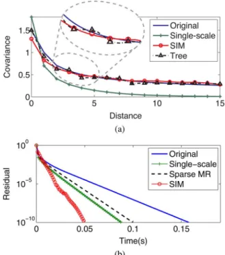
Fig. 12. (a) Covariance behavior of various models. (b) Comparison of infer-ence performance for polynomially decaying covariance experiments.
the original and the single-scale approximation is where is the number of variables.
C. Polynomially Decaying Covariance for A 2-D Gaussian Field
We consider a collection of 256 Gaussian random variables arranged spatially on a grid. The variance of each vari-able is given by and the covariance between each pair
of variables is given by , where is
the spatial distance between nodes and . The original graph-ical structure (corresponding to the inverse of the specified co-variance matrix) is fully connected, and the single-scale approx-imation of it is still densely connected with each node connected to at least 31 neighbors.
Fig. 11 shows theconjugategraph of the SIM model approxi-mation within each scale, i.e., the sparsity of the conditional co-variance at that scale. We emphasize that these conjugate edges encode the in-scale conditional correlation structure among the variables directly, so each node is onlylocallycorrelated when conditioned on other scales. Fig. 12(a) displays the covariance as a function of the distance between a pair of nodes. The co-variance of the single-scale approximation falls off much more rapidly than that of the original model, and the magnified por-tion of the plot emphasizes the blocky artifacts of the tree model.
TABLE III
POLYNOMIALLYDECAYINGCOVARIANCEAPPROXIMATION
We conclude that our SIM model provides good modeling ca-pabilities for processes with long-range correlation.
To compare the inference performance, we generate random noisy measurements using the specified statistics and compare the computation time to solve the inference problem for the SIM model (using the inference algorithm in Section IV-B), the original and the single-scale approximate model (using the ET algorithm described in Section IV-A), and the sparse MR model (using the algorithm in [8]). Table III shows the average time until convergence (the relative residual error reaches ) averaged over 100 experiments, and Fig. 12(b) shows the residual error versus computation time for one set of random measurements.12The SIM modeling approach provides a
sig-nificant gain in convergence rate over the other models. Note that the sparse MR model has a smaller number of parameters, but the divergence and the average time until convergence are larger. Hence, even though sparse MR models have advantages over single-scale approximations, SIM models provide more accurate approximations of the underlying process and enable more efficient inference procedures.
VII. CONCLUSION ANDFUTUREWORK
In this paper, we have introduced a new class of Gaussian MR models with sparse in-scale conditional covariance structure at each scale and tree-structured connections across scales. In our SIM model, each variable is correlated with only a few other variables in the same scale when conditioned on other scales. Our approach overcomes the limitations of tree-structured MR models and provides good modeling performance especially in capturing long-range covariance behavior without blocky arti-facts. In addition, by decomposing the information matrix of the resulting MR model into the sum of a sparse matrix (the infor-mation matrix corresponding to interscale graphical structure) and an information matrix that has a sparse inverse (the in-scale conditional covariance), we develop an efficient inference algo-rithm utilizing the sparsity in both Markov and covariance struc-ture. Our algorithm alternates computations across scales using the sparse interscale graphical structure, and in-scale computa-tions that reduce to sparse matrix multiplicacomputa-tions.
We also describe a method for learning models with this struc-ture, i.e., for building SIM models that provide a good approx-imation to a target covariance. Given a target covariance at the finest scale, our learning algorithm first constructs an exact MR model for the target covariance, and then optimizes the struc-ture of each scale using log-determinant maximization to obtain
12The computation time was measured at AMD Opteron 270 Dual Core
a sparse conjugate graph approximation. In Appendix I, we in-troduce one method to construct an exact MR model, which first learns a good MR tree model and then augments each scale in a coarse-to-fine way. An important and interesting extension of our learning method would be to alternatively optimize the tree and the in-scale models in a computationally tractable way. Al-though for simplicity we assumed that the interscale structure of SIM models is a tree, our inference procedure is efficient for the more general case of having a sparse interscale structure (but not necessarily a tree) as well.
SIM models are of most value when there are long-distance correlations, which are most prominent in multidimensional data such as in geophysical fields, and the application of our methods in such areas is a promising line of work. While our focus in this paper is on the Gaussian model, applying similar principles to discrete or other more general models is also of interest. Although the sparse matrix multiplication and the log-det optimization framework for Gaussian models are not directly applicable to the discrete case, we expect that having a sparse in-scale dependency structure at each scale condi-tioned on other scales may still result in efficient inference and learning algorithms.
APPENDIXI
COMPUTING THETARGETINFORMATIONMATRIX OF ANMR MODEL
Suppose that we are given a target covariance of the vari-ables at the finest scale. In this section, we discuss a method to introduce hidden variables at coarser scales and build anexact
MR model, so that when we marginalize out all coarser scale variables, the marginal covariance at the finest scale is exactly equal to . The information matrix of this exact MR model can be used as the target information matrix in (10) to obtain a SIM model approximation.
To begin with, we learn an interscale model by selecting a tree structure (without any in-scale connections) withadditional hiddenvariables at coarser scales and the original variables at the finest scale. Selecting a good tree structure is important, but this structure does not need to be perfect since we later aug-ment the interscale model with in-scale structures. For some processes, there exists a natural hierarchical structure: for ex-ample, for regular 1-D or 2-D processes, the MR tree models in Fig. 1 can be used. For other problems in which the spatial re-lation among the variables is not clearly defined, we can group variables that are highly correlated and insert one coarser scale variable for each group. Once the structure is fixed, the EM al-gorithm [5] can be applied to choose the parameters that best match the given target covariance for the finest scale vari-ables. This procedure is efficient for a tree-structured model.
After the parameter fitting, we have an information matrix corresponding to an MR tree model. Although the EM al-gorithm will adjust the elements of so that the marginal covariance at the finest scale is close to , it will in general not match the cross-correlation between variables at different finest scale nodes. As mentioned in Section V-C, if we view as a first approximation to , it has a structure as in Fig. 5 except that the in-scale conditional structure that we have learned (the
shaded blocks in in the figure) isdiagonalrather than full, resulting in artifacts that correspond to inaccurate matching of finest scale cross covariances. As a result, the basic idea of our construction is to recursively modify our approximation to , from coarse-to-fine scales to get full matching of marginal sta-tistics at the finest scale.
In an MR tree model, the covariance matrix at each scale can be represented in terms of the covariance at the next finer scale (11) where and are determined by .13 Since we wish
to modify the tree model so that the covariance matrix at the finest scale becomes , we set for the finest scale and compute a target marginal covariance for each scale in afine-to-coarseway using (11). These target marginal covari-ances at each scale can be used to modify . Specifically, the diagonal matrix of the tree model is replaced with a nondi-agonal matrix so that themarginalcovariance at scale is equal to , the target marginal covariance at that scale computed using (11). In modifying , we proceed in acoarse-to-fineway. Suppose that we have replaced through , and let us consider computing . We partition the information matrix of the resulting MR model into nine submatrices with the in-scale information matrix at scale at the center14:
(12)
Note that except for , all submatrices are equivalent to the cor-responding components in because we have only replaced coarser in-scale blocks.
From (12), the marginal covariance at scale is
. By setting this equal to the target covariance matrix in (11), the target information matrix at scale can be computed as follows:
(13) which we replace with in (12) and proceeds to the next finer scale until we reach the finest scale. The matrix inversion in the above equation requires computation that is cubic in the number of variables . Learning a graphical model structure typically involves at least computation [1], so computing is not a bottleneck of the learning process.
After the algorithm augments in-scale structures for all scales, the resulting information matrix has the marginal covari-ance at the finest scale exactly equal to the target covaricovari-ance matrix . In addition, has dense in-scale structure both as a graphical model and in terms of the corresponding conjugate graph (since in general the matrix is not sparse and does not have a sparse inverse), and a sparse interscale graphical struc-ture. Hence, the information matrix can be used as the target
13LetB = (J ) andD = (J ) . Then,A = B D
andQ = D 0 B D B .
14Form = 1(the coarsest scale) andm = M(the finest scale), the partition
consists of only four submatrices. Also, the 0-blocks in (12) are immediate be-cause of the MR structure, which does not have edges directly between scales m 0 1andm + 1.
TABLE IV
LEARNINGALGORITHM INDETAIL
information matrix of the MR model in (10) with the -norm dropped from the objective function to learn a SIM model ap-proximation.
APPENDIXII
SEQUENTIALSTRUCTUREOPTIMIZATION
In Appendix I, we constructed an exact MR model such that the marginal covariance at the finest scale matches the specified target covariance exactly. The information matrix of the exact MR model can be used as the target information matrix in (10) to learn a SIM model approximation. In this section, we intro-duce an alternative approach to learn a SIM model; instead of first constructing an exact MR model across all scales and then optimizing the structure of all scales in parallel by solving (10), one can interleave the procedure of finding a target information matrix at scale and optimizing its structure to have a sparse conjugate graph.
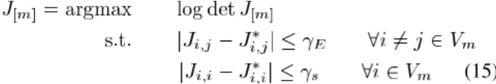
After computing the target information matrix at scale using (13) (before proceeding to compute at the next finer scale), we perform structure optimization at scale to ob-tain a sparse in-scale conditional covariance approximation (i.e., a sparse conjugate graph). This in-scale structure optimization can be performed by solving a simplified version of the log-det problem in (10). Since the interscale edges of are sparse by our construction, the -norm can be dropped from the objective function of (10). In addition, the parameters at all scales other than scale are fixed. Thus, the optimization problem reduces to the following:
(14) where is the set of nodes at scale . Using the approxima-tion techniques described in Appendix III, the above problem can be solved more efficiently than the problem in (10) that does not use the sequential approach.
APPENDIXIII
COMPUTATIONAL SIMPLIFICATIONS IN SOLVING THELOG-DETPROBLEM
In this section, we introduce some techniques to obtain an ap-proximate solution of the log-determinant problem in (14) effi-ciently, and provide a method for choosing the regularization
parameters. The problems in (10) and (14) are both convex and can be solved using standard convex optimization techniques [4]. In order to further reduce the computational complexity, we ignore the positive–definiteness condition until we find a solution that maximizes the log-determinant with the element-wise constraints satisfied. Then, the problem reduces to (9) that involves only the information matrix at scale , which can be efficiently solved using the techniques in [1], [17], and [21]. If, after replacing with the solution , the entire infor-mation matrix is positive–definite, then is indeed the op-timal solution. If is not positive–definite, then we adjust the regularization parameter, and for this purpose, we allow two reg-ularization parameters: one for all nodes and one for all edges
(15) where and are parameters for edges and nodes, respec-tively. Note that the KKT conditions of the above problem are exactly the same as those in Proposition 1, and the inverse of
(the conjugate graph at scale ) is sparse.
It is straightforward to show that the optimal solution of (15) has the diagonal elements equal to , so for large enough value of becomes positive–definite. Therefore, if the resulting is not positive–definite, we can increase the value of . In practice, we set equal to where is the maximum value of the off-diagonal elements of , and set the initial value of for all coarser scales. For the finest scale, we use and adjust so that the divergence between the approximate and target distribution is minimized.
After every scale in the MR model is augmented with a sparse conjugate graph, the resulting SIM model has a sparse interscale structure, and a sparse conjugate graph at each scale. Table IV summarizes the algorithm for learning a SIM model given the target covariance at the finest scale.
ACKNOWLEDGMENT
The authors would like to thank Prof. H. Chen for helpful discussions about the stock returns example.
REFERENCES
[1] O. Banerjee, L. E. Ghaoui, A. D’Aspremont, and G. Natsoulis, “Convex optimization techniques for fitting sparse Gaussian graphical models,” inProc. 23rd Annu. Int. Conf. Mach. Learn., 2006, pp. 89–96. [2] C. M. Bishop, Pattern Recognition and Machine Learning. New
York: Springer-Verlag, 2006.
[3] C. A. Bouman and M. Shapiro, “A multiscale random field model for Bayesian image segmentation,”IEEE Trans. Image Process., vol. 3, no. 2, pp. 162–177, Mar. 1994.
[4] S. Boyd and L. Vandenberghe, Convex Optimization. Cambridge, U.K.: Cambridge Univ. Press, 2004.
[5] W. L. Briggs, A Multigrid Tutorial. Philadelphia, PA: SIAM, 1987. [6] V. Chandrasekaran, J. K. Johnson, and A. S. Willsky, “Estimation in
Gaussian graphical models using tractable subgraphs: A walk-sum analysis,”IEEE Trans. Signal Process., vol. 56, no. 5, pp. 1916–1930, May 2008.
[7] M. J. Choi, V. Chandrasekaran, and A. S. Willsky, “Maximum entropy relaxation for mutiscale graphical model selection,” inProc. IEEE Int. Conf. Acoust. Speech Signal Process., Apr. 2008, pp. 1889–1892. [8] M. J. Choi and A. S. Willsky, “Multiscale Gaussian graphical models
and algorithms for large-scale inference,” inProc. IEEE Statist. Signal Process. Workshop, Aug. 2007, pp. 229–233.
[9] M. J. Choi, V. Chandrasekaran, and A. S. Willsky, “Exploiting sparse Markov and covariance structure in multiresolution models,” inProc. 26th Annu. Int. Conf. Mach. Learn., 2009, pp. 177–184.
[10] K. C. Chou, A. S. Willsky, and A. Benveniste, “Multiscale recursive estimation, data fusion, and regularization,”IEEE Trans. Autom. Con-trol, vol. 39, no. 3, pp. 464–478, Mar. 1994.
[11] M. L. Comer and E. J. Delp, “Segmentation of textured images using a multiresolution Gaussian autoregressive model,”IEEE Trans. Image Process., vol. 8, no. 3, pp. 408–420, Mar. 1999.
[12] D. R. Cox and N. Wermuth, Multivariate Dependencies: Models, Anal-ysis and Interpretation. London, U.K.: Chapman & Hall/CRC, 1996. [13] C. Crick and A. Pfeffer, “Loppy belief propagation as a basis for com-munication in sensor networks,” inProc. 19th Conf. Uncertainty Artif. Intell., 2003, pp. 159–166.
[14] M. S. Crouse, R. D. Nowak, and R. G. Baraniuk, “Wavelet-based sta-tistical signal processing using hidden Markov models,”IEEE Trans. Signal Process., vol. 46, no. 4, pp. 886–902, Apr. 1998.
[15] V. Delouille, R. Neelamani, and R. Baraniuk, “Robust distributed esti-mation using the embedded subgraphs algorithm,”IEEE Trans. Signal Process., vol. 54, no. 8, pp. 2998–3010, Aug. 2006.
[16] M. Drton and M. D. Perlman, “Model selection for Gaussian concen-tration graphs,”Biometrika, vol. 91, no. 3, pp. 591–602, 2004. [17] J. Friedman, T. Hastie, and R. Tibshirani, “Sparse inverse covariance
estimation with the graphical lasso,”Biostatistics, vol. 9, no. 3, pp. 432–441, 2008.
[18] G. H. Golub and C. H. Van Loan, Matrix Computations. Baltimore, MD: The Johns Hopkins Univ. Press, 1990.
[19] C. Graffigne, F. Heitz, P. Perez, F. Prêteux, M. Sigelle, and J. Zerubia, “Hierarchical Markov random field models applied to image analysis: A review,” inSPIE Conference Series. Bellingham, WA: SPIE, 1995, vol. 2568, pp. 2–17.
[20] L. Greengard and V. Rokhlin, “A fast algorithm for particle simula-tions,”J. Comput. Phys., vol. 73, no. 2, pp. 325–348, 1987.
[21] J. K. Johnson, V. Chandrasekaran, and A. S. Willsky, “Learning Markov structure by maximum entropy relaxation,” inProc. 11th Int. Conf. Artif. Intell. Statist., Mar. 2007.
[22] A. Kannan, M. Ostendorf, W. C. Karl, D. A. Castanon, and R. K. Fish, “ML parameter estimation of multiscale stochastic processes using the EM algorithm,”IEEE Trans. Signal Process., vol. 48, no. 6, pp. 1836–1847, Jun. 2000.
[23] Z. Kato, M. Berthod, and J. Zerubia, “Multiscale Markov random field models for parallel image classification,” inProc. Int. Conf. Comput. Vis., May 1993, pp. 253–257.
[24] G. Kauermann, “On a dualization of graphical Gaussian models,” Scan-dinavian J. Statist., vol. 23, pp. 105–116, 1996.
[25] A. J. Krener, R. Frezza, and B. C. Levy, “Gaussian reciprocal pro-cesses and self-adjoint stochastic differential equations of second order,”Stochastics Stochastics Rep., vol. 34, pp. 29–56, Jun. 1991. [26] S. L. Lauritzen, Graphical Models. Oxford, U.K.: Oxford Univ.
Press, 1996.
[27] S. Lee, V. Ganapathi, and D. Koller, “Efficient structure learning of Markov networks usingl regularization,” inAdvances in Neural Infor-mation Processing Systems (NIPS) 19. Cambridge, MA: MIT Press, 2007.
[28] J. Li, R. M. Gray, and R. A. Olshen, “Multiresolution image classifi-cation by hierarchical modeling with two-dimensional hidden Markov models,”IEEE Trans. Inf. Theory, vol. 46, no. 5, pp. 1826–1841, Aug. 2000.
[29] J. Löfberg, “Yalmip: A toolbox for modeling and optimiza-tion in MATLAB,” in Proc. Comput.-Aided Control Syst. De-sign Conf., 2004, pp. 284–289 [Online]. Available: http://con-trol.ee.ethz.ch/joloef/yalmip.php
[30] B. B. Mandelbrot and J. W. Van Ness, “Fractional Brownian motions, fractional noises and applications,”SIAM Rev., vol. 10, pp. 422–437, 1968.
[31] R. Neal and G. Hinton, “A view of the EM algorithm that justifies incre-mental, sparse, and other variants,” inLearning in Graphical Models, M. I. Jordan, Ed. Cambridge, MA: MIT Press, 1999, pp. 355–368.
[32] S. Osindero and G. Hinton, “Modeling image patches with a directed hierarchy of Markov random fields,” inAdvances in Neural Informa-tion Processing Systems (NIPS) 20. Cambridge, MA: MIT Press, 2008.
[33] E. B. Sudderth, M. J. Wainwright, and A. S. Willsky, “Embedded trees: Estimation of Gaussian processes on graphs with cycles,”IEEE Trans. Signal Process., vol. 52, no. 11, pp. 3136–3150, Nov. 2004. [34] A. S. Willsky, “Multiresolution Markov models for signal and image
processing,”Proc. IEEE, vol. 90, no. 8, pp. 1396–1458, Aug. 2002.
Myung Jin Choi(S’06) received the B.S. degree in electrical engineering and computer science from Seoul National University, Seoul, Korea, in 2005 and the S.M. degree in electrical engineering and computer science from the Massachusetts Institute of Technology (MIT), Cambridge, in 2007, where she is currently working towards the Ph.D. degree with the Stochastic Systems Group.
She is a Samsung scholarship recipient. Her re-search interests include statistical signal processing, graphical models, and multiresolution algorithms.
Venkat Chandrasekaran(S’03) received the B.S. degree in electrical engineering and the B.A. degree in mathematics from Rice University, Houston, TX, in 2005 and the S.M. degree in electrical engineering from the Massachusetts Institute of Technology, Cambridge, in 2007, where he is currently working towards the Ph.D. degree with the Stochastic Sys-tems Group.
His research interests include statistical signal processing, optimization methods, machine learning, and computational harmonic analysis.
Alan S. Willsky (S’70–M’73–SM’82–F’86) received the S.B. and Ph.D. degrees from the Department of Aeronautics and Astronautics, Mass-achusetts Institute of Technology (MIT), Cambridge, in 1969 and 1973, respectively.
He joined the MIT faculty, in 1973 and is the Edwin Sibley Webster Professor of Electrical Engineering and Director of the Laboratory for Information and Decision Systems. He was a founder of Alphatech, Inc. and Chief Scientific Consultant, a role in which he continues at BAE Systems Advanced Information Technologies. From 1998 to 2002, he served on the U.S. Air Force Scientific Advisory Board. He has delivered numerous keynote addresses and is coauthor of the textSignals and Systems(Englewood Cliffs, NJ: Prentice-Hall, 1996). His research interests are in the development and application of advanced methods of estimation, machine learning, and statistical signal and image processing.
Dr. Willsky received several awards including the 1975 American Automatic Control Council Donald P. Eckman Award, the 1979 ASCE Alfred Noble Prize, the 1980 IEEE Browder J. Thompson Memorial Award, the IEEE Control Sys-tems Society Distinguished Member Award in 1988, the 2004 IEEE Donald G. Fink Prize Paper Award, and Doctorat Honoris Causa from Universit de Rennes in 2005. He and his students, colleagues, and postdoctoral associates have also received a variety of Best Paper Awards at various conferences and for papers in journals, including the 2001 IEEE Conference on Computer Vision and Pattern Recognition, the 2003 Spring Meeting of the American Geophysical Union, the 2004 Neural Information Processing Symposium, Fusion 2005, and the 2008 award from the journal Signal Processing for the outstanding paper in the year 2007.