P
ROBABILISTIC
N
ETWORK
A
NALYSIS
P
HILIPPAP
ATTISON ANDG
ARRYR
OBINSINTRODUCTION
The aim of this chapter is to describe the foun-dations of probabilistic network theory. We re-view the development of the field from an early reliance on simple random graph models to the construction of progressively more realistic mod-els for human social networks. Hence, we show how developments in probabilistic network mod-els are increasingly able to inform our under-standing of the emergence and structure of social networks in a wide variety of settings.
SOCIAL
NETWORKS
Growing numbers of social scientists from an increasingly diverse set of disciplines are turn-ing their attention to the study of social net-works. The precise reasons vary, but almost certainly, there are at least two key factors at work. The first is an increasing recognition that networks matter in many realms of social, litical, and economic life. Networks both po-tentiate and constrain the social interactions that, for instance, underpin the dissemination of knowledge, the exercise of power and influence, and the transmission of communicable diseases. Ignoring the structured nature of these inter-actions often leads to erroneous conclusions
about their consequences, as social scientists from a number of disciplines have repeatedly pointed out (e.g., Bearman, Moody, & Stovel, 2004; Kretzschmar & Morris, 1996). The second reason for a heightened focus on social networks is our increasing capacity to measure, monitor, and model social networks and their evolution through time and hence to draw social networks into a more general program for a quantitative so-cial science. Probabilistic models for soso-cial net-works have played—and will likely increasingly play—a vital role in these developments. In this chapter, we review the progress in attempts to de-velop probabilistic network models and point to areas of ongoing development.
WHAT
IS
DISTINCTIVE
ABOUT
MODELS FOR
SOCIAL
NETWORKS?
At the outset, it is important to recognize that so-cial networks pose particular challenges as far as probability modeling is concerned. Unlike obser-vations on a set of distinct actors, where an as-sumption of independent observations may often seem reasonable, social relationships are much less plausibly regarded as independent. Rela-tional observations may share one or more ac-tors and hence be subject to influences such as the goals and constraints of a particular actor.
Alternatively, they may be linked by other rela-tionships (e.g., the relationship between actors i and j may be linked with the relationship be-tween actors k and l by a relationship involving actors j and k) and hence dependent, for example, by virtue of competition or cooperation regard-ing relational resources involvregard-ing actors j and k. As we see below, the development of probabilis-tic network models began with simple models that assumed independent relational ties, but em-pirical researchers quickly confronted the prob-lem that social networks appeared to deviate from simple random structures in seemingly system-atic ways. Hence, the story of the development of probabilistic network models is a story of al-ternatively probing and parameterizing progres-sively more complex systematicities in network structure.
NOTATION AND
SOME
BASIC
PROPERTIES OF
GRAPHS
AND
DIRECTED
GRAPHS
We begin with some notations and some important definitions, referring the reader to Wasserman and Faust (1994); see also Bollobás (1998) for a fuller exposition of key concepts.
Graphs and Directed Graphs
We let N =1,2,...,n be a set of network
nodes, with each node representing a social actor. The actors are often persons but may also be groups, organizations, or other social entities. An observed social network may be represented
as a graph G = (N,E) comprising the node set
N and the edge set E comprising all pairs (i,j) of distinct actors who are linked by a network tie. The tie, or edge,(i,j) is said to be incident with nodes i and j. In this case, the network ties are taken to be nondirected, with no distinction between the tie from actor i to actor j and the tie from actor j to actor i; in other words, the edges (i,j) and (j,i) are regarded as indistin-guishable. If it is desirable to distinguish these ties—as it often is—the network may be
repre-sented instead by a directed graph(N,E)on N:
The node set is then also N, and the arc set E is the set of all ordered pairs(i,j)such that there is
a tie from actor i to actor j. The convention of us-ing the term edge in the case of a nonordered pair (i.e., a nondirectional tie) and arc in the case of an ordered pair (i.e., a directional tie) is widely adopted by graph theorists, although network researchers are inclined to use the term tie inter-changeably in both cases. In many cases, by con-vention, ties of the form(i,i), known as loops, are excluded from consideration.
Graphs and directed graphs can be conve-niently represented by a graph drawing. The ele-ments of the node set N are represented by points in the drawing, and a nondirected line connects
node i and node j if(i,j)is an edge in the edge
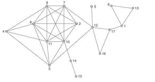
set E. In the case of a directed graph, an arc rep-resented by a directed arrow is drawn from node i to node j if(i,j)is in the arc set E.Figures 18.1 and 18.2 show examples of a graph and a directed graph, respectively.
Order, Size, and Density
The order and size of a graph are defined to be the number of nodes and edges, respectively; likewise, the order and size of a directed graph are the number of nodes and arcs, respectively. For example, the graph in Figure 18.1 has order 17 and size 34; the directed graph in Figure 18.2 has order 37 and size 169. The size of a graph of order n varies between 0 for an empty graph and n(n−1)/2 for the complete graph of order n (i.e., the graph in which every pair of nodes is linked by an edge). For a directed graph of order n, size
varies between 0 and n(n−1). The density of a
graph or directed graph is a ratio of its actual size to the maximum possible size for n nodes, and it is in the range [0, 1]. The densities of the graph and directed graph of Figures 18.1 and 18.2 are 0.25 and 0.13, respectively.
Adjacency Matrix
Graphs and directed graphs can be represented by a binary adjacency matrix. For example, in the
case of a graph, we can define x to be an n×n
ma-trix with entries xi j=1 if there is an edge between
i and j and xi j=0 otherwise. Since xi j=1 if and
only if xji=1, x is necessarily a symmetric
ma-trix. In the case of a directed graph, unit entries in x correspond to arcs in E (i.e., xi j=1 if and only if
8 11 10 2 12 17 16 1 13 6 5 7 9 14 15 3 4
Figure 18.1 A graph on 17 nodes (mutual friendship network).
Figure 18.2 A directed graph on 37 nodes (reported collaboration network).
there is an arc from i to j, and xi j=0 otherwise).
In this case, symmetry is not necessarily implied. The adjacency matrix corresponding to the graph
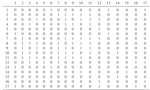
of Figure 18.1 is shown inTable 18.1. Note that
the size of a graph is x++/2, whereas the size of a directed graph is x++, where x++=∑i jxi jis the
sum of entries in the adjacency matrix.
Degree, Degree Sequence,
and Degree Distribution
The number k(i) of edges incident with a
given node i is termed its degree: k(i) =∑jxi j
is the sum of row i in the adjacency matrix x. The degree sequence (k(1),k(2),... ,k(n)) of a
Table 18.1 Adjacency Matrix for Graph of Figure 18.1 1 2 3 4 5 6 7 8 9 10 11 12 13 14 15 16 17 1 0 0 0 0 0 1 0 0 0 0 0 0 1 0 0 0 1 2 0 0 0 0 0 0 1 1 1 1 1 0 0 0 0 0 0 3 0 0 0 1 0 0 0 1 0 1 1 1 0 0 0 0 0 4 0 0 1 0 0 0 0 1 1 0 1 0 0 0 0 0 0 5 0 0 0 0 0 0 0 0 0 0 0 1 0 0 0 0 0 6 1 0 0 0 0 0 0 0 0 0 0 0 1 0 0 0 0 7 0 1 0 0 0 0 0 1 1 1 1 1 0 0 0 0 0 8 0 1 1 1 0 0 1 0 1 1 1 0 0 0 0 0 0 9 0 1 0 1 0 0 1 1 0 1 1 0 0 0 0 0 0 10 0 1 1 0 0 0 1 1 1 0 1 0 0 1 0 0 0 11 0 1 1 1 0 0 1 1 1 1 0 0 0 0 0 0 0 12 0 0 1 0 1 0 1 0 0 0 0 0 0 0 0 1 1 13 1 0 0 0 0 1 0 0 0 0 0 0 0 0 0 0 0 14 0 0 0 0 0 0 0 0 0 1 0 0 0 0 1 0 0 15 0 0 0 0 0 0 0 0 0 0 0 0 0 1 0 0 0 16 0 0 0 0 0 0 0 0 0 0 0 1 0 0 0 0 1 17 1 0 0 0 0 0 0 0 0 0 0 1 0 0 0 1 0
graph is the sequence of the degrees of its nodes,
indexed by the labels 1,2,...,n of nodes in
N. The degree distribution is (d0,d1,...,dn−1),
where dk is the number of nodes in G of
de-gree k. For example, the dede-gree distribution of the
graph in Figure 18.1 is shown inFigure 18.3. In
a directed graph, the concept of degree is more complex, since there may be an arc directed from node j toward a given node i or away from node i toward node j, or there may be arcs in both direc-tions between nodes i and j. We therefore char-acterize each node i in a directed graph by its out-degree outi=xi+=∑jxi j, indegree ini=x+i=
∑jxji, and mutual degree muti=∑jxi jxji.
Subgraphs and the Dyad and Triad Census
Each subset S of the node set N of a graph G=
(N,E) gives rise to an induced subgraph H of
G with node set S and edge set E containing all edges in G that link pairs of nodes in S. More
gen-erally, any graph H= (N,E)is a subgraph of G
if N⊆N and E⊆E. For example, the subgraph induced by the node set 1, 6, 13 of the graph of Figure 18.1 has edge set (1, 6),(1, 13),(6, 13); the graph comprising the node set 1, 6, 13 and the edge set (1, 6),(1, 13) is a subgraph of the graph of Figure 18.1 but not an induced subgraph. If
every pair of nodes in the subgraph H is con-nected by an edge, then H is said to be a clique; for example, the subgraph induced by 2, 7, 8, 9, 10, 11 in Figure 18.1 is a clique of order 6.
A useful set of descriptive statistics for a graph or directed graph is a summary of the form of all of its small subgraphs. For example, the dyad census is a count of the number of each possi-ble type of two-node induced subgraphs, and the triad census is the set of counts of three-node induced subgraphs. For example, the graph of Figure 18.1 has 102 null dyads and 34 linked dyads; its triad census comprises 279, 322, 49, and 30 induced three-node subgraphs with zero, one, two, and three edges, respectively. The dyad census and the triad census for directed graphs are defined similarly, but the number of forms of two-node and three-node subgraphs is greater in the directed graph case.
Implicit in the description of the dyad and triad census is the notion that two graphs (or sub-graphs) can have the same form. We can make this notion more explicit by defining an isomor-phic mapping between graphs. Specifically, two
graphs G= (N,E)and H= (N,E)are
isomor-phic if there is a one-to-one mappingϕ from N onto Nsuch that(i,j)is an edge in E if and only if(ϕ(i),ϕ(j))is an edge in E.
4 3 2 1 0 Frequency Mean =4.00 Std. Dev. =2.15058 N=17 Degree 0.00 2.00 4.00 6.00 8.00
Figure 18.3 The degree distribution for the mutual friendship graph.
Paths, Reachability, and Connectedness
Social networks are often important to under-stand because social processes—such as the dif-fusion of information, the exercise of influence, and the spread of disease—are potentiated by net-work ties. Not surprisingly, therefore, pathlike structures in networks that might be associated with the flow of social processes are important concepts. A path from node i to node j is an ordered sequence i=i0,i1,...,il = j of distinct
nodes in which each adjacent pair (ij−1,ij) is
linked by an edge or an arc. The length of the path is l. If there is a path from a node i to a node j, then j is said to be reachable from i. If node j is the same as node i, then the path is termed a cycle of length l.
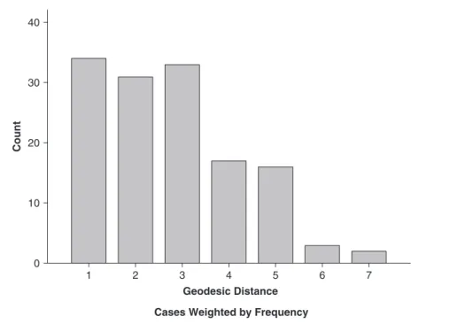
A geodesic from node i to another node j is a path of minimum length, and the geodesic dis-tance di jfrom node i to node j is the length of the
geodesic. If there is no path from i to j, the geo-desic distance is infinite. The geogeo-desic distance
di j for distinct nodes i and j is either an
inte-ger in the range from 1 to n−1 or infinite. For
a graph, geodesic distances are symmetric, that is dji=di j; this is not necessarily the case however,
for directed graphs. The geodesic distribution of a graph or directed graph is the distribution of fre-quencies of geodesic distances—that is, the dis-tribution of counts of the number of ordered pairs of nodes having each possible geodesic distance. The geodesic distribution of the graph of Figure
18.1 is presented inFigure 18.4 in the form of a
histogram. The geodesic distribution can be seen as a useful summary of internode distances. Later, we refer to the quartiles of this distribution as sim-ple summary statistics for internode distances.
If each node in a graph G is reachable from each other node, then G is connected. A compo-nent of G is a maximal connected subgraph—that is, a connected subgraph with vertex set W for which no larger set Z containing W is connected. The graph of Figure 18.1 is clearly connected.
In the case of a directed graph, we may also define a semipath from node i to node j as an ordered sequence i=i0,i1,...,il= j of distinct
nodes in which either(ij−1,ij)or(ij,ij−1)is an arc. The length of the semipath is m. If each node in a directed graph G is reachable from each other node, then G is strongly connected. If there is a semipath from each node in G to each other node, then G is said to be weakly connected.
1 40 30 20 0 10 2 3 4 5 6 7 Geodesic Distance Cases Weighted by Frequency
Count
Figure 18.4 Geodesic distribution for the mutual friendship graph.
SIMPLE
RANDOM
GRAPHS
AND
DIRECTED
GRAPHS
The Hungarian mathematicians Paul Erd˝os and Alfréd Rényi initiated an important approach to the study of random graph structures with a foundational series of papers beginning in 1959 (Erd˝os & Rényi, 1959). They introduced two pri-mary random graph distributions on a fixed node
set N=1,2,...,n. The probability distributions
are defined on the set of all graphs on n distinct nodes; this set contains 2n(n−1)/2 graphs, since
each of the n(n−1)/2 pairs of nodes may or
may not be linked by an edge. Each of the two random graph distributions that we introduce be-low associates a probability with every graph in this set.
G
(
n
,
p
)
In the first case, the edges of a graph are re-garded as a set of independent Bernoulli
vari-ables. If we let Xi j denote the edge variable for
the pair of nodes i and j and p be the (uni-form) probability that the edge between i and j
is present, then we can write Pr(Xi j =1) = p
and, hence, Pr(Xi j=0) =1−p. Since the edge
variables are independent, it is then easy to write down the probability of any particular graph H of order n and size m:
Pr(G=H) =pm(1−p)m∗−m,
where m∗=n(n−1)/2 is the maximum
num-ber of edges in a graph of order n. The set of all possible graphs of order n and their correspond-ing probabilities is the random graph distribution
G(n,p).
In the special case where p=0.5, the
proba-bility of each graph H on n nodes is
Pr(G=H) = (0.5)m(0.5)m∗−m= (0.5)m∗, and hence, every graph on n nodes is equiproba-ble. This distribution is often termed the uniform random graph distribution and is denoted by U .
G
(
n
,
m
)
The second random graph distribution asso-ciates nonzero probabilities only with graphs of order n and size m; furthermore, every such graph is assumed to be equiprobable. Since there are
n!/(m!(n−m)!)distinct graphs in the class, the probability of any particular graph of order n and size m is
Pr(G=H) =m!(n−m)!/n!.
The distribution G(n,m) may be regarded
as the uniform random graph distribution on n nodes, conditional on the property of having m
edges. It may also be designated U |x++ =m.
More generally, we can define a conditional uni-form random graph distribution in terms of any
graph property Q (Bollobás, 1985). If Q is a
subset of all possible graphs on n nodes, then
the distribution U| Qassigns equal probabilities
(viz., 1/| Q |) to all graphs in the subsetQand
zero probability to all graphs not inQ. We term
U| Qthe uniform random graph distribution
con-ditional onQ.
Some Results for Simple Random Graphs
The field of random graphs in G(n,p) and
G(n,m) has grown rapidly since its inception.
Much work has explored the features of vari-ous random graph classes, particularly as n be-comes large, and the way in which these features change, often very rapidly, as a function of p. Bollobás (1998) contains an excellent introduc-tion to the field, as does the review by Albert and Barabási (2002); here, we illustrate just two aspects of this literature by considering the ex-pected values of some statistics inG(n,p)and by reviewing properties of a graph as a function of p inG(n,p).
We begin by determining the expected number of cliques in a graph. Let Ys=Ys(G)be the
num-ber of cliques of order s in the graph G. Then, the
expected value of Yscan readily be computed as
E(Ys) = (n!/[s!(n−s)!])pu,
where u=s(s−1)/2 is the number of edges in
a clique of order s (e.g., see Bollobás, 1998). In
G(17,0.25), for example, the expected number of cliques of order 3 is 10.6, and the expected num-ber of cliques of order 4 is 0.58. The graph of Figure 18.1 has 17 nodes and a density of 0.25, and it is therefore interesting to compare the ex-pected values forG(17,0.25)with those observed for the graph of Figure 18.1—namely, 34 cliques of order 3 and 18 cliques of order 4.
Indeed, if F is any subgraph with s nodes and t edges and YF is the number of subgraphs of G
that are isomorphic to F, then the expected value
of YFcan readily be shown to be
E(YF) = (n!/[(n−s)!a])pt,
where a is the number of distinct ways in which the nodes of the graph F can be labeled with the
integers 1,2,...,s to yield the same graph. For
example, in the case of a cycle of order s, F has s edges and s nodes, and there are 2s distinct ways in which nodes can be labeled to yield the same graph; hence,
E(YF) = (n!/[(n−s)!2s])ps.
The expected number of induced subgraphs iso-morphic to F may be similarly derived:
E(YF) = (n!/[(n−s)!a])pt(1−p)s(s−1)/2−t.
The latter formula may be used, for example, to compute the expected triad census for a graph of a given order and density.
The expression for the expected number of
subgraphs isomorphic to F inG(n,p)allows us
to explore features of random graphs as n tends to infinity. Since
E(YF) = (n!/[(n−s)!a])pt≈nspt/a,
it is clear that if p=cn−s/t, then E(YF)≈ct/a
and the expected number of subgraphs
isomor-phic to F, denoted byλ =ct/a, is a finite
num-ber. If, however, pns/t tends to 0 or ∞ as n
tends to ∞, then the probability that a random
graph in G(n,p) contains at least one subgraph
F converges to 0 or 1, respectively (e.g., Albert & Barabási, 2002). Thus, p=cn−s/t is a criti-cal probability below which graphs with large n rarely contain F and above which they almost certainly do. An important set of results in ran-dom graph theory documents the many graph properties that show this form of rapid transition from being very unlikely to very likely as a func-tion of the edge probability p.
Application of this approach allows us to in-fer for large n some expected features of random graphs inG(n,p)as a function of p, relative to n.
graph inG(n,p)comprises a number of compo-nents, each without any cycles; if p lies between 1/n and(ln n)/n, then almost every graph has a so-called giant component (i.e., a component in-cluding a large proportion of the nodes in N); and if p>(ln n)/n, then almost every graph is con-nected (e.g., see Albert & Barabási, 2002).
Random directed graph distributions may be similarly defined, though interest in them has largely come from social scientists with applica-tions to network data in mind. It is to this litera-ture that we now turn.
APPLICATIONS OF
RANDOM
GRAPH
AND
DIRECTED
GRAPH
DISTRIBUTIONS
TO
SOCIAL
NETWORK
DATA
Before describing the application of random graphs to social networks, it is important to say something about typical sources of social net-work data (e.g., Wasserman & Faust, 1994). A common method of measuring social networks is to survey all members of a circumscribed popu-lation about their ties. In this case, ties are typ-ically directional, and there may or may not be a limit imposed on the maximum number of ties reported by each respondent. Occasionally in this case, it is fruitful to consider the graph con-structed from mutual ties only. For example, the graph of Figure 18.1 is the set of mutual ties observed among the girls in a Grade 8/9 high school class, obtained in response to the question “Who are your best friends in the class?” Net-works are also commonly inferred from archival data, such as communication logs or membership or attendance lists. Less common strategies in-clude direct observation and more elaborate sur-vey techniques.
Application of Directed
Random Graph Distributions
In the 1930s, the psychiatrist Jacob Moreno and colleagues reported using random directed graph distributions to compute quantities such as the expected number of mutual ties (i.e., ∑i,jXi jXji/2), where Xi jdenotes the random
vari-able for the tie from node i to node j. Moreno and colleagues also calculated properties of the
inde-gree distribution in a random directed graph dis-tribution (see, e.g., the very interesting historical account in Freeman, 2004).
Consider, for example, the random graph dis-tributionDG(n,p)with a fixed set of n nodes and uniform but unknown arc probability p; this is the
directed graph analog of G(n,p). The expected
number of mutual ties for directed graphs in this
distribution is n(n−1)p2/2, and the expected
number of nodes with indegree k is npk(1−
p)n−1−k. If a social network with n nodes and
x++=∑i jxi j arcs has been observed, then the
arc probability p can be estimated from the net-work data as p∗=x++/(n[n−1]). This estimate of the arc probability can be used to compute the expected number of mutual ties and the expected number of nodes with each possible indegree k, on the assumption that the observed network was
generated from DG(n,p∗). These expected
val-ues can be compared with the observed number of mutual ties and the observed indegree distribu-tion in the network x. If the observed values are markedly different from the expected ones, then it can be argued that there is reason to question the suitability of the assumption of independent random arcs with uniform probability that under-pinned the computation of expected values.
The computations by Moreno and colleagues revealed what would later become a very com-mon finding: that the observed number of mutual ties in an observed human social network is much greater than the number expected on the basis of arc probability alone and the indegree distribu-tion is more heterogeneous than expected—that is, there are more nodes with very low and very high indegree than expected. These and similar findings suggest that tendencies toward mutuality and heterogeneity in partner “attractiveness” are systematic features of observed social networks comprising ties of affiliation.
Most important for our purposes here, Moreno introduced the idea of using random directed graph distributions as null distributions. The fea-tures of this null distribution could be compared with features of an observed network, a compar-ison enabling researchers to identify the ways in which the observed network appeared to be sys-tematically different. In this early example, and in many to follow, it was important that the ex-pected features of the null distribution could be
derived mathematically. Much later, when fast computers and more versatile simulation algo-rithms were introduced, this restriction could be relaxed, but it was an important reason for the focus of early applications on this “null distribu-tion” approach. Moreover, although this early ap-plication assumed very simple null distributions (such as independent arcs with uniform tie proba-bility), more complex distributions were soon de-veloped. Indeed, the strategy continues to be used in new ways (e.g., Bearman et al., 2004; Pattison, Wasserman, Robins, & Kanfer, 2000) and to be re-discovered in new fields (e.g., Milo et al., 2002). It remains an important means by which some of the systematic structural properties of human so-cial networks can be and have been uncovered.
Holland, Leinhardt, and colleagues were re-sponsible for developing a number of important elaborations of this basic strategy. For exam-ple, Holland and Leinhardt (1975) computed the expected mean vector and variance-covariance matrix for the triad census in the uniform random
directed graph distribution U|mut, asym, null1
conditional on fixed numbers mut, asym, and null of mutual, asymmetric, and null ties, respec-tively (mut = ∑i jxi jxji/2, asym = ∑i j[xi j(1−
xji) +xji(1−xi j)], null = ∑i j(1−xi j)(1−xji)).
In other words, they computed the expected dis-tribution of the triad census while conditioning on the dyad census. This allowed them to con-struct a test statistic for any linear combination of triad counts and, hence, assess whether the ob-served combination of triad counts is in the upper or lower tail of the expected distribution. For ex-ample, they could test for the presence of transi-tivity (i.e., the property that arcs from nodes i to j and from j to k are accompanied by an arc from i to k).
Similar calculations can be made for other distributions of possible interest, including the
uniform distribution U | {xi+},mut conditional
on the outdegrees of each node in the directed graph as well as the number of mutual ties. Of course, for some desirable combinations, such as U | {xi+},{x+i},mut, the calculations
are very difficult and have prompted alterna-1In fact, Holland and Leinhardt (1975) termed this the U| MAN distribution, but we have attempted to keep notation consistent in the chapter.
tive parametric approaches. In some of these difficult cases, clever simulation strategies have been devised to circumvent the difficult math-ematics. For example, Snijders (1991) used an
importance-sampling approach to simulate U |
{xi+},{x+i}, and McDonald, Smith, and Forster
(2007) have described a Markov chain Monte
Carlo algorithm to simulate the distribution U|
{xi+},{x+i}, mut.
BIASED
NETS
One other early probabilistic approach deserves mention. In a series of papers, Rapoport and colleagues developed the theory of biased nets— that is, random networks with biases toward symmetry, transitivity, and other features charac-teristic of observed social networks (Rapoport, 1957). Although a full and satisfactory mathe-matical treatment proved elusive, Rapoport and colleagues employed their conceptualization of biased nets to conduct some illuminating stud-ies of the connectivity structure of a large friend-ship network (e.g., Rapoport & Horvath, 1961). In part, their work can be seen as the intellec-tual precursor to the more general probabilis-tic developments described below, but a differ-ent framing of the “biases” has proved more useful.
THE
p
1MODEL
Comparison of observed social networks with random directed graph distributions consistently revealed a greater than expected number of mutual ties and greater than expected degree het-erogeneity. As a consequence, it was felt desir-able to compare observed networks with graph distributions that resembled observed networks in these fundamental respects. The problem of satisfactorily simulating the random graph dis-tribution conditional on the number of mutual ties and the in-degree and out-degree sequences is arguably still not resolved. In the meantime, Holland and Leinhardt (1981) developed an alter-native approach: a probability model that param-eterized these tendencies. This model was an
important step toward the development of a more general framework.
The p1 model developed by Holland and
Leinhardt (1981) assumes independent dyads Di j= (Xi j,Xji). The distribution of the entire
net-work X= [Xi j]can then be determined by
spec-ifying the probability of each possible dyadic
form for Di j since the probability of the entire
network X is the product of the dyad probabili-ties. The individual dyad probabilities can be ex-pressed in terms of the probability of occurrence of a mutual dyad, an asymmetric dyad, and a null dyad. Thus, we define
Pr(Di j= (1,1)) =mi j=mji,
Pr(Di j= (1,0)) =ai j, and
Pr(Di j= (0,0)) =ni j=nji,
where mi j+ai j+aji+ni j=1 for all i=j.
The resulting probability distribution Pr(X=x) =
∏
i<j mXi jXjii j∏
i=j aXi ji j (1−X ji)∏
i<j n(i j1−Xi j)(1−X ji)may then be reexpressed in the exponential form Pr(X=x) =K exp[
∑
i<j
ρi jXi jXji+
∑
i jθi jXi j],
where, for all i=j,
• ρi j =log{mi jni j/(ai jaji)} is an index of
reciprocity,
• θi j=log{ai j/ni j}is a log-odds measure of
the probability of an asymmetric dyad be-tween i and j, and
• K = ∏i<j[1/(1+ exp(θi j) +exp(θji) +
exp(ρi j +θi j +θji))] is a normalizing
quantity.
Holland and Leinhardt added two useful restrictions to this general dyad-independent model. The first was that the reciprocity param-eterρi jis a constant for all dyads; that is,ρi j=ρ
for all i= j. The second was that the parameter
θi jdepended additively on the propensity of arcs
to emanate from node i and the propensity of arcs to have node j as a target; in other words,
θi j=θ+αi+βj, for i=j.
The resulting model is termed the p1model:
p1(x) =Pr(X=x) =K exp ρ
∑
i,j Xi jXji+θX++ +∑
i αiXi++∑
i βiX+i .The parametersρandθcan be interpreted as
uni-form reciprocity and density parameters, and the
node-dependent parametersαi andβi reflect the
expansiveness and attractiveness, respectively, of each node i.
The development of the p1model was an
im-portant step in probabilistic network theory, not the least because much of the machinery of sta-tistical modeling could be brought to bear on the problem of assessing model adequacy. The model could be estimated from data, and its goodness of fit could be subjected to careful scrutiny, as Brieger (1981) demonstrated. Such scrutiny led to the recognition that observed networks often exhibited structural properties not captured by
the parameters of the p1model and spawned the
development of two important lines of further model development.
LATENT
V
ARIABLEMODELS
The first line of development is a series of la-tent variable models in which the assumption of independent dyads is replaced by an assumption of independent dyads conditional on unobserved variables representing some potential underlying structure.
One such model was inspired by the concept of structural equivalence in a graph (Lorrain & White, 1971). Two nodes are structurally equiv-alent if they have identical patterns of relation-ships to other nodes. The concept of structural equivalence has been very influential in the so-cial networks literature because it can be used to represent the idea that two actors have the same social position in a network; that is, that they are indistinguishable from a relational point of view. Formally, two nodes i and j are structurally equivalent in a directed graph G with adjacency matrix x if xik=xjk and xki=xk j for all nodes
be partitioned into blocks. Nowicki and Snijders (2001) assumed that the blocks to which nodes belong are unobserved. They defined a set of independent and identically distributed latent
random variables Z = [Zi], where Zi denotes
the block of node i and Pr(Zi =k) =θk. They
assumed the dyads Di j = (Xi j,Xji) to be
con-ditionally independent given the blocks and the probability that a dyad has a particular relational form to depend only on the (unobserved) blocks of the nodes. In other words,
Pr(Di j=a|Z=z) =ηa(zi,zj),
where a is a vector of possible values for the
dyad, with a∈ {(1,1),(1,0),(0,1),(0,0)}for a directed graph anda∈ {(1,1),(0,0)}for a graph, andηa(zi,zj)is the block-dependent probability
of observing the vectora.
In this model, two nodes i and j are stochasti-cally equivalent if they belong to the same block
and hence the same dyad probabilities (Pr(Dik=
a|Z=z) =Pr(Djk=a|Z=z)) for all nodes
k. Since the dyads are assumed to be condition-ally independent given the blocks Z, the joint
distribution of the Di jgiven Z is the product of
the conditional dyad probabilities. Nowicki and Snijders (2001) developed a Bayesian approach
to the estimation ofθandηand, hence, the
com-putation of the posterior probabilities that any pair of nodes are in the same block and that a dyad has any particular relational form.
Several other important latent variable mod-els have been developed for particular types of social networks that are likely to reflect some form of proximity among actors, such as friend-ship or collaboration. In cases such as these, it may be reasonable to assume that tie probabilities are monotonically related to proximity in a latent space. For example, Hoff, Raftery, and Handcock (2002) proposed a model that assumes that nodes have latent locations in some low-dimensional Euclidean space and that given these latent locations, tie variables are conditionally indepen-dent. Schweinberger and Snijders (2003) devel-oped a similar model based on an ultrametric rather than Euclidean space; in their model, every pair of nodes is associated with an unobserved distance in an ultrametric space corresponding to a discrete hierarchy of “settings,” and tie proba-bilities are conditionally independent given these
latent ultrametric distances. (Distances in an ul-trametric space satisfy the ulul-trametric inequality; i.e., d(i,j)max{d(i,k),d(j,k)}for any triple
of nodes i,j,k.) They developed approaches for
estimating the unobserved ultrametric distances. Handcock, Raftery, and Tantrum (2005) have re-cently extended Hoff et al.’s (2002) model by as-suming that the latent locations are drawn from a finite mixture of multivariate normal distribu-tions, each of which represents a different group of nodes.
MARKOV
RANDOM
GRAPHS
The second recent line of development has been to build probabilistic network models in which conditional dependencies among tie variables are permitted. This work began with the recognition by Frank and Strauss (1986) that a general ap-proach for modeling interactive systems of vari-ables (Besag, 1974) could be usefully applied to the problem of modeling systems of interdepen-dent network tie variables on a fixed set of nodes. This was an important step because it permitted models to go beyond the limiting assumption of dyad independence in quite a general way. Frank and Strauss (1986) introduced a Markov depen-dence assumption for network tie variables: Two network tie variables were assumed to be condi-tionally independent given the values of all other network tie variables, unless they had a node in common. Thus, whereas a tie between nodes i and j was assumed to be conditionally indepen-dent of ties involving all other distinct pairs of nodes k and l, it could be conditionally dependent on any other ties involving i and/or j.
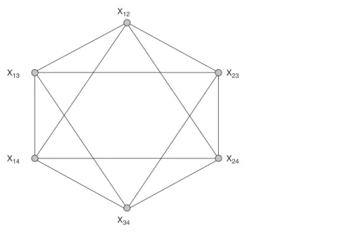
Assumptions about which pairs of tie vari-ables are conditionally dependent, given the val-ues of all other tie variables, can be represented as a dependence graph. The node set of the depen-dence graph D is the set of tie variables{Xi j},
and two tie variables are joined by an edge in D if they are assumed to be conditionally depen-dent given the values of all other tie variables. In the case ofG(n,p), D is an empty graph since all pairs of variables are assumed to be mutually
in-dependent. In the Markov case, the variable Xi j
is connected to Xikand Xjk for all k=i or j, and
X12 X34 X23 X24 X13 X14
Figure 18.5 Dependence graph for a Markov random graph on four nodes.
shows the Markov dependence graph for a ran-dom graph of order 4.
As Frank and Strauss originally outlined, the consequences of any proposed assumptions about potential conditional dependencies among net-work tie variables can be inferred from the Hammersley-Clifford theorem (Besag, 1974). The theorem establishes a model for the inter-acting system of tie variables in terms of param-eters that pertain to the presence or absence of certain configural forms in the network. The model, known as an exponential random graph model, takes the general form
Pr(X=x) =exp
∑
A γAzA(x) /κ,where A is a subset of tie variables (defining a
potential network configuration),γA is a model
parameter associated with the configuration A (to be estimated) and is nonzero only if the subset A
is a clique in the dependence graph D, zA(x) =
∏Xi j∈Axi jis the sufficient statistic corresponding
to the parameterγAand indicates whether or not
all tie variables in the configuration A have
val-ues of 1 in the network x, andκis a normalizing
quantity.
To reduce the number of model parameters, Frank and Strauss (1986) introduced a homo-geneity constraint that parameters for isomorphic configurations are equal. With this constraint, there is a single parameterγ[A]for each class[A]
of isomorphic configurations that correspond to cliques in the dependence graph. The sufficient statistic in the model corresponding to the class [A] is then
Z[A](x) =
∑
A∈[A]Xi j∏
∈Axi j,
that is, a count of all observed configurations in the graph x that are isomorphic to the configu-ration corresponding to A. For example, in the case of a homogeneous Markov random graph, it is readily seen that cliques A in the dependence graph D correspond to graph configurations that
are edges, stars, and triangles (seeFigure 18.6),
and the model therefore takes the form Pr(X=x)
=exp(θL(x) +
∑
k
σkSk(x) +τT(x))/κ,
where L(x), Sk(x), and T(x)are the number of
edges, k-stars(2kn−1), and triangles in
the network x andθ,σk(2kn−1), andτare
k Nodes
Triangle
k-Star
Edge
Figure 18.6 Markov model configurations: edges, stars, and triangles.
In many circumstances, the parameters may be interpreted by observing that if a configura-tion class [A] has a large positive (or negative) parameter in the model, then the presence of many configurations in the class enhances (or reduces) the likelihood of the overall network, net of the effect of all other configurations. It should be noted, though, that the function relating the value
of one of the model’s parameters, say λ[A], to
the expected value of the corresponding sufficient
statistic z[A](x)may be markedly nonlinear and
exhibit a sharp and rapid transition from lower average counts to higher average counts, with a relatively small change in the parameter (holding constant the values of all other model parameters). For example, the expected number of triangles in
a graph as a function of the triangle parameterτ
is shown for a graph on 17 nodes inFigure 18.7.
The values of the parametersθ,σ2, andσ3 are
fixed at−1.2558,−0.0451, and−0.1084,
respec-tively, andτtakes values in the range [0.05, 1.70].
Figure 18.7 shows the distribution of the triangle statistic in the form of a box plot for each value of
τ. It can be seen that for low values ofτ, small
in-creases inτare associated with small and steady
increases in the triangle statistic. Asτapproaches
1.40, though, the impact of small changes inτ
in-creases rapidly in magnitude, and there is a sharp transition to a higher value of the triangle tic. Near the point of transition, the triangle statis-tic may take values typical of the graphs on either side of this apparent threshold. This form of non-linear relationship is common, and the location of this threshold and the sharpness of the rise in the region of greatest sensitivity are likely to depend on other parameter values.
It is important to emphasize that even though this model is well understood in the case where
only the parameter θ is nonzero (since this
is just the model G(n,p) with p =exp(θ)/
[1+exp(θ)]), more complex instantiations can
be seen as models for self-organizing network processes (Robins, Pattison, & Woolcock, 2005). Robins et al. (2005) have demonstrated that specific sets of parameter values for the homo-geneous Markov model can characterize very di-verse network structures, including small worlds, caveman worlds, long-path worlds, and so on.
For some parameter values, the model may ac-cord very high probability to a small set of graphs and very low probability to the rest, as Handcock (2004) and Snijders (2002) have demonstrated. Handcock termed these models near-degenerate. For detailed investigation of the behavior of spe-cific models, see Handcock (2004), as well as Park and Newman (2004) and Burda, Jurkiewicz, and Krzywicki (2004).
Model Simulation
To understand properties such as near-degeneracy of the exponential random graph model Pr(X = x) = exp(∑AγAzA(x))/κ, it is
helpful to be able to simulate it efficiently (i.e.,
to draw graphs x with probability Pr(X=x)),
and this generally means circumventing the need
to compute the normalizing quantityκ, sinceκ
is a function of all graphs in the distribution. As Strauss (1986) and others have observed, the Metropolis algorithm can be used for this pur-pose. The algorithm sets up a Markov chain on the space of all possible graphs of order n in such
Tau 150 125 100 75 50 25 0 Triangles 0.05 0.10 0.15 0.20 0.25 0.30 0.35 0.40 0.45 0.50 0.55 0.60 0.65 0.70 0.75 0.80 0.85 0.90 0.95 1.00 1.05 1.10 1.15 1.20 1.25 1.30 1.35 1.40 1.45 1.50 1.55 1.60 1.65 1.70
Figure 18.7 Boxplots for the triangle statistic as a function of the triangle parameter for a Markov model on a graph of 17 nodes (θ=−1.2558,σ2=−0.0451,σ3=−0.1084,τbetween 0.00 and 1.75).
a way that the Markov chain has the model as its stationary distribution. It may be described as follows:
1. Begin with some graph x.
2. At each step, select an edge at random, say the(i,j)edge, and let x be the graph that is identical to x, except that the edge from i to j is switched to absent if it is present in x or to present if it is absent in x.
3. Replace x by x with probability min[1,
exp{∑AγA(zA(x)−zA(x)}].
4. Return to Step 2, unless some specified tar-get number of steps has been taken.
To sample from Pr(X=x), it is usual to
be-gin sampling graphs from the chain after some initial number of steps have been completed (the burn-in period); graphs are then sampled at a rate
that may depend on n. Many variations of this approach may also be used; a valuable discussion may be found in Snijders (2002).
Estimation of Model Parameters
In many settings, primary interest lies in esti-mating exponential random graph model param-eters from observed network data. For example, given the graph of Figure 18.1, there may be in-terest in estimating the parameters of a Markov model from which it might have been generated. In the early applications of these models to ob-served data, an approximate form of estimation known as pseudolikelihood estimation was of-ten used (Strauss & Ikeda, 1990; Wasserman & Pattison, 1996), even though the properties of the estimates were not well understood. Initial attempts to apply the very promising approach of Markov chain Monte Carlo maximum likeli-hood estimation (MCMCMLE) were not always
successful because the properties of the models under consideration were not always fully appre-ciated, as Snijders (2002) and Handcock (2004) demonstrated. However, with a growing under-standing of model properties and more careful at-tention to model adequacy, substantial progress has now been made in implementing MCM-CMLE approaches (see Handcock, Hunter, Butts, Goodreau, & Morris, 2004; Snijders, 2002).
As an example of MCMCMLE, we estimate the parameters of the model
Pr(X=x)
=exp(θL(x) +σ2S2(x) +σ3S3(x) +τT(x))
κ
for the mutual friendship network of Figure 18.1 using the approach proposed by Snijders (2002). The resulting estimates and estimated standard
errors for the parameters θ, σ2, σ3, and τ are
shown in Table 18.2.2 Also displayed in Table
18.2 are convergence t statistics, computed as the difference between the observed value of the suf-ficient statistic for a parameter and its average simulated value, divided by the standard devia-tion of simulated values. If the estimated value is indeed the maximum likelihood estimate, the simulated values should be centered on the ob-served value and the t statistics should all be small, preferably below 0.1 (Snijders, 2002). It can be seen from Table 18.2 that the t statis-tics satisfy this requirement. Although the edge, 2-star, and 3-star parameters are negative and within about 1 standard error of 0, the triangle parameter is positive and approximately seven times its estimated error. This suggests that, other graph features (edges, 2-stars, and 3-stars) being equal, graphs with more triangles are more likely. That such a model is needed for the graph of Figure 18.1 is consistent with the earlier compu-tations based on G(17, 0.25).
Goodness of Fit
A good statistical model should not be un-necessarily complex, but it should be adequate: 2The estimation was conducted using PNet (Wang, Robins, & Pattison, 2006), an implementation of the estimation ap-proach in Snijders (2002). Retrieved from http://www.sna. unimelb.edu.au/pnetpnet.html.
that is, the data should resemble realizations from the model in many important respects. We can assess model adequacy by comparing the ob-served network with graphs generated by the model in features that are not necessarily param-eterized within the model. What is important in such comparisons is very much a function of the modeling context, but there are often good reasons to require that the model captures the degree of clustering in a network, the distribu-tion of degrees, and the connectivity structure that is represented by the geodesic distribution (e.g., Goodreau, 2007; Robins, Snijders, Wang, Handcock, & Pattison, 2007). It is important to note that only some of these characteristics need be associated with model parameters; others might be seen as consequences of these param-eterized tendencies.
For example, if we simulate the model Pr(X=x)
=exp(θL(x) +σ2S2(x) +σ3S3(x) +τT(x))
κ
using the parameter estimates in Table 18.2, we can not only compare the observed graph with the simulated graph in terms of its sufficient statistics (viz., the number of edges, 2-stars, 3-stars, and triangles), but we can also make the comparison in relation to any unmodeled network character-istic, such as the number of nodes of degree 4 or more, the number of geodesic distances of length 3, and so on.
Table 18.3 summarizes these comparisons for the graph of Figure 18.1 and the parameter es-timates of Table 18.2. It can be seen that the t statistics are all less than 1 for
• the local clustering coefficient (the average across all nodes i of the proportion of pairs
of nodes j and k incident with i(xi j =1=
xik)that are themselves connected(xjk=1),
• the global clustering coefficient (the pro-portion of the triples of nodes{i,j,k}with xi j=1=xikfor which xjk=1),
• the standard deviation of the degree distri-bution, and
• the skewness coefficient of the degree distri-bution.
Table 18.2 MCMCMLEs for Markov Model of the Graph of Figure 18.1 Parameter Estimate s. e. t Edge −1.2558 1.3561 0.047 2-Star −0.0451 0.3551 0.060 3-Star −0.1084 0.0974 0.073 Triangle 1.4438 0.2073 0.058
Table 18.3 Goodness of Fit for Markov Model for the Mutual Friendship Network (Figure 18.1) Simulated
Observed Mean Std dev t
Edges 34 34.07 8.91 −0.0077 2-Stars 139 138.35 77.45 0.0084 3-Stars 181 178.05 156.49 0.0189 Triangles 30 29.34 28.39 0.0231 Std dev degrees 2.09 1.71 0.46 0.8296 Skew degrees 0.08 −0.26 0.62 0.5480 Global clustering 0.65 0.54 0.21 0.5246 Mean local clustering 0.64 0.47 0.19 0.4917 Variance local clustering 0.14 0.10 0.04 0.9899
The observed graph, in other words, exhibits levels of clustering and degree heterogeneity that fall within the envelope of values expected for the model. The 1st, 2nd, and 3rd quartiles of the observed geodesic distribution are 1, 3, and 4, respectively; the median values for the distribu-tion of these quartiles across simuladistribu-tions were 2, 2, and 4, suggesting that the model is associated with somewhat more homogeneous internode
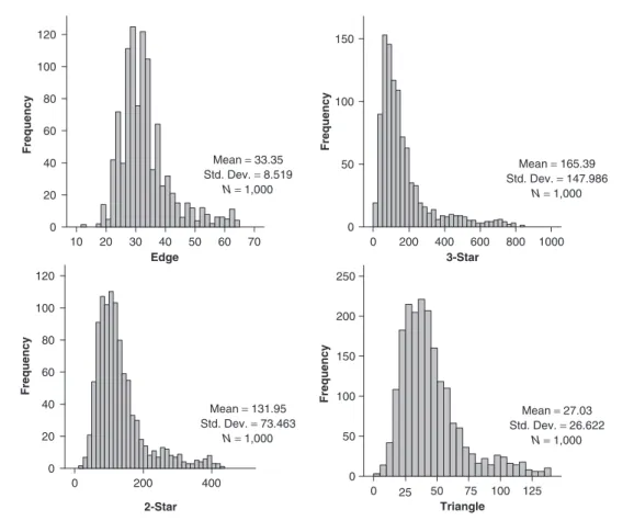
dis-tances than the data. InFigure 18.8, the
distri-butions of the number of edges, 2-stars, 3-stars, and triangles for the Markov random graph model with these parameter values are shown. While the mean of each distribution is close to the observed value for the Figure 18.1 graph, as expected, it can be seen that the distributions are positively skewed. Indeed, Figure 18.7 shows the impact on one of these statistics—the number of triangles—
of changing its corresponding parameter valueτ
while holding all other parameters constant. It can be seen from Figure 18.7 that the estimated value of 1.4438 is very close to the point of transition be-tween low and high values of the triangle statistic and the positively skewed distribution of the trian-gle statistic is consistent with the estimated value
ofτbeing just below this point.
Related Model Parameters
In the Markov model just fitted, parameters for 2-stars and 3-stars were included, but parameters for higher-order stars (4-stars, 5-stars, and so on) were assumed to be 0. Arguably, fitting higher-order star parameters might be desirable, because more star parameters will lead to better char-acterizations of the degree distribution for the network. Indeed, Snijders, Pattison, Robins, and Handcock (2006) proposed that all star param-eters be used, but they also imposed a hypothesis about the relationships among stars parameters. Specifically, they assumed that
σk+1= (−1/λ)σk,
for k>1 andλ1 a (fixed) constant,
a hypothesis they termed the alternating k-star hypothesis. It follows from this hypothesis that
∑
k σkSk(x) =∑
k (−1)kSk(x)/λk−2 σ2 and, hence, that the entire set of starlike terms in the model can be captured by a single star param-eter (σ2) with a single alternating k-star statistic:10 120 150 100 50 0 0 200 400 600 800 1000 100 80 60 40 20 0 20 30 40 Edge Frequency Frequency 50 60 70 Mean = 33.35 Std. Dev. = 8.519 N= 1,000 Mean = 165.39 Std. Dev. = 147.986 N= 1,000 Mean = 27.03 Std. Dev. = 26.622 N= 1,000 Mean = 131.95 Std. Dev. = 73.463 N= 1,000 0 120 100 80 60 40 20 0 200 400 2-Star 3-Star Frequency 0 250 200 150 100 50 0 50 75 25 100 125 Triangle Frequency
Figure 18.8 Distribution of edge, 2-star, 3-star, and triangle statistics in the Markov random graph distribution with parametersθ=−1.2558,σ2=−0.0451,σ3=−0.1084,τ=1.4438.
S[λ](x) =
∑
k
(−1)kSk(x)/λk−2
It is of course an empirical matter whether this is an appropriate hypothesis to make. This expres-sion can be simplified to yield a simpler form of the alternating k-star statistic:
S[λ](x) =λ2
∑
i
{(1−1/λ)k(i)+k(i)/λ−1}, recalling that k(i)denotes the degree of node i.3
Fitting the model
Pr(X=x) =exp(θL(x) +σ2S[λ](x))/κ 3Hunter and Handcock (2006) proposed an alternative statis-tic based on geometrically weighted degree statisstatis-tics; the re-sulting model is equivalent, provided that the edge parameter is included.
to the friendship network in Figure 18.1 yields
estimates (standard errors) of−2.7454 (1.3794)
and 0.4822 (0.4098) forθ andσ2, respectively
(as before,θis an edge parameter, and L(x), the
number of edges in the network x, is its sufficient statistic). Although this model does a reasonable job in reproducing the standard deviation and the skewness coefficient for the degree distribution, not surprisingly, it does a poor job in recover-ing network clusterrecover-ing. We present a better-fittrecover-ing model below.
In some applications to date (e.g., Goodreau,
2007; Snijders et al., 2006), a fixed value ofλ
(such as 2) has been assumed; Hunter and
Hand-cock (2006) have shown that λ can be treated
as a variable within a curved exponential family model, and they have developed an associated es-timation method.
REALIZATION-DEPENDENT
MODELS
A critique of the Markov dependence assump-tion led Pattison and Robins (2002) to construct a more general class of “realization-dependent” network models. They argued that conditional de-pendencies among tie variables may emerge from the network processes themselves, with new de-pendencies created as network ties are generated.For instance, Xi j and Xkl might become
condi-tionally dependent if there is an observed tie be-tween, say, j and k. Baddeley and Möller (1989) termed such models realization dependent.
The 4-Cycle Hypothesis
Snijders et al. (2006) argued that in addition to
the Markov assumption, two network ties, Xi jand
Xkl, might be conditionally dependent in the case
where there is an observed tie between, say, j and k and between l and i; that is, if the presence of a tie from i to j and from k to l would create a 4-cycle in the graph. The rationale for this assump-tion is that a 4-cycle is a closed structure that can sustain mutual social monitoring and influ-ence, as well as levels of trustworthiness within which obligations and expectations might prolif-erate (e.g., Coleman, 1988).
Snijders et al. (2006) showed that this assump-tion led to addiassump-tional nonzero parameters in an exponential random graph model, including those referring to collections of 2-paths with common starting and ending nodes and collections of
tri-angles with a common base (see Figure 18.9).
We define a k-2-path to be a subgraph comprising two nodes, i and j, and a set of k paths of length 2 from i to j through distinct intermediate nodes
m1,m2,...,mk. A k-triangle is a subgraph
com-prising two connected nodes, i and j, and a set of k paths of length 2 from i to j through distinct intermediate nodes m1,m2,...,mk. If we letνkbe
the model parameter associated with a k-2-path
andτkthe parameter associated with a k-triangle,
we can entertain assumptions about the relation-ships among related parameters (as in the case of k-stars earlier)—namely,
νk+1=−νk/λ and
τk+1=−τk/λ.
As for the star parameters, this is just a hy-pothesis, and its adequacy needs to be assessed. Under this assumption, the statistics
U[λ](x) =
∑
k (−1)kUk(x)/λk−2 and T[λ](x) =∑
k (−1)kTk(x)/λk−2become single statistics associated with the
parametersν1 andτ1, respectively, where Uk(x)
and Tk(x) are the number of 2-paths and
k-triangles in the network x. It should be noted that
the value of λ need not be the same for each
statistic; as before, Hunter and Handcock have shown how to estimate these parameters.
The parameter estimates presented in Table 18.4 are for a model fitted to the mutual
friend-ship network of Figure 18.1. The positiveτ1
esti-mate suggests that networks with relatively many triangles are more likely, other statistics being equal, with the cumulative impact of multiple tri-angles with a common base pair of nodes dimin-ishing as the number of such triangles increases.
Likewise, the negativeν1estimate suggests that
networks with relatively few 2-paths among a pair of nonconnected nodes are more likely, other statistics being equal. Both of these effects are consistent with a pressure toward closure for mu-tual friendship ties.
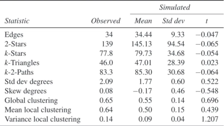
The goodness of fit for this model is sum-marized in Table 18.5. The median values of the quartiles of the geodesic distribution for the random graph distribution simulated from the parameter estimates in Table 18.4 are 2, 3, and 5, suggesting better recovery of short distances than the Markov model, though not of longer ones. Overall, the model of Table 18.4 appears to do a reasonably good job of characterizing the fea-tures of the mutual friendship network.
Directed Graph Models
The derivation of similar classes of models for directed graphs is, in principle, very similar to the derivation of models for their nondirected counterparts. Directed graphs give rise, how-ever, to substantially more complicated param-eterizations, as a comparison between triadic
k Nodes
k Nodes
k Nodes
Figure 18.9 The k-star, k-2-path, and k-triangle.
Table 18.4 MCMCMLEs for Realization-Dependent Exponential Random Graph Model for the Mutual Friendship Network (Figure 18.1)
Parameter estimate s.e. t Edge −0.0354 1.7851 −0.037 2-Star −0.0520 0.1094 −0.038 k-Star 0.0674 0.8689 −0.040 k-Triangles 0.7250 0.3159 −0.043 k-2-Paths −0.5583 0.1727 −0.025
Table 18.5 Goodness of Fit of Realization-Dependent Model for the Mutual Friendship Network Simulated
Statistic Observed Mean Std dev t
Edges 34 34.44 9.33 −0.047 2-Stars 139 145.13 94.54 −0.065 k-Stars 77.8 79.73 34.68 −0.054 k-Triangles 46.0 47.01 28.39 0.023 k-2-Paths 83.3 85.30 30.68 −0.064 Std dev degrees 2.09 1.77 0.60 0.522 Skew degrees 0.08 −0.17 0.46 −0.548 Global clustering 0.65 0.55 0.14 0.696 Mean local clustering 0.64 0.50 0.15 0.439 Variance local clustering 0.14 0.09 0.04 1.207
forms in graphs and directed graphs quickly sug-gests. There are, as a result, some subtleties to the development of models in the directed graph case (see Robins, Pattison, & Wang, 2006, for further details).
Exogenous Covariates
The general modeling framework can read-ily accommodate covariates at the node or dyad level, and, of course, if such covariates are re-garded as important influences on network tie formation, then they should be included in mod-els for the network. For example, a general and systematic approach to the inclusion of node-level covariates has been outlined by Robins, Elliott, and Pattison (2001), who extended the dependence graph formulation described ear-lier to include directed dependence relationships from exogenous node-level variables to endoge-nous tie variables. These developments offer an important means for exploring a wide range of in-teresting interactions among actor-level and net-work tie variables, including homophily effects (e.g., McPherson, Smith-Lovin, & Cook, 2001) and the effects of spatial locations (e.g., Butts, 2003; Wong, Pattison, & Robins, 2006).
EXTENSIONS
There are a variety of ways in which the models just described may be extended to incorporate richer data forms, including multiple networks, longitudinal data, and changing node and tie sets. In addition, some initial progress has been made on the problem of dealing with missing data. We do not have space for a full account of these in-teresting and important developments but point to some key developments in each case.
The development of probabilistic models for graphs and directed graphs has been loosely shadowed by the construction of a parallel, al-beit generally later, set of models for multiple networks measured on a common node set. Mul-tivariate exponential random graph models are described by Pattison and Wasserman (1999); see also Koehly and Pattison (2005).
Although networks are often measured at a single point in time, they are, in reality, dynamic entities, and there is considerable interest in
the processes that underpin their evolution. An important line of work has developed continuous-time Markov process models for network evolu-tion (e.g., see Snijders, 2001). More recently, this framework has been extended to accommodate the possibility of co-evolutionary mechanisms by which network tie change depends on and con-tributes to change in node atcon-tributes (Snijders, Steglich, & Schweinberger, 2007).
CONCLUSION
The field of probabilistic network theory has progressed rapidly in the past 10 years, and as Goodreau (2007) and Robins et al. (2007) have cogently demonstrated, it is now possible to build plausible models for many small and large so-cial networks. Undoubtedly, experience with the current generation of realization-dependent net-work models will lead to further improvements in model specification and a clearer understand-ing of how the content of network ties and the contexts in which they are observed might inform model building. Perhaps most important though, the field has now advanced to the point where the promise of a step-change in our understanding of social processes on networks and their conse-quences might be realized.
ACKNOWLEDGMENTS
We are grateful to Peng Wang and Galina Daraganova for helpful comments on this chapter.
REFERENCES
Albert, R., & Barabási, A. (2002). Statistical mechanics of complex networks. Reviews of Modern Physics, 74, 47–97.
Baddeley, A., & Möller. (1989). Nearest-neighbor Markov point processes and random sets. Interna-tional Statistical Review, 57, 89–121.
Bearman, P., Moody, J., & Stovel, K. (2004). Chains of affection: The structure of adolescent romantic and sexual networks. American Journal of Sociology, 110, 44–91.