Comparison of variance estimation methods for use with
two-dimensional systematic sampling of land use/land cover data
Linda Aune-Lundberg, Geir-Harald Strand
*Norwegian Forest and Landscape Institute, P.O.Box 115, N-1431 Ås, Norway
a r t i c l e i n f o
Article history:Received 3 April 2014 Received in revised form 26 June 2014
Accepted 3 July 2014 Available online 5 August 2014 Keywords:
Systematic sample Spatial sampling Uncertainty Variance Land cover Land use
Area frame survey Spatial autocorrelation
a b s t r a c t
Systematic sampling is more precise than simple random sampling when spatial autocorrelation is present and the sampling effort is equal, but there is no unbiased method to estimate the variance from a systematic sample. The objective of this paper is to assess selected variance estimation methods and evaluate the influence of spatial structure on the results. These methods are treated as models and a complete enumeration of Norway was used as the modeling environment. The paper demonstrates that the advantage of systematic sampling is closely related to autocorrelation in the material, but also that the improvement is influenced by periodicity and drift in the variables. Variance estimation by
strati-fication with the smallest possible strata gave the best overall results but may underestimate the vari-ance when spatial autocorrelation is absent. Treating the sample as a simple random sample is a safe and conservative alternative when spatial autocorrelation is absent or unknown.
©2014 The Authors. Published by Elsevier Ltd. This is an open access article under the CC BY-NC-ND license (http://creativecommons.org/licenses/by-nc-nd/3.0/).
1. Introduction
Spatial sampling surveys fill an important gap between the
traditional, labor-intensive wall-to-wallfield survey and the effi
-cient, but in many cases rather inaccurate mapping by remote
sensing (Wyatt, 2000; Verburg et al., 2011). The approach is used
from the global down to the sub-national level. The Food and Agriculture Organization of the United Nations used systematic sampling together with satellite remote sensing for their Global
Forest Resources Assessment 2010 (FAO, 2010). This approach
reduced the amount of image processing and allowed FAO to involve national experts who revised the sample areas. The
com-bination of field inventories and systematic sampling was also
chosen when the European statistical agency (Eurostat) developed the LUCAS (Land use/cover area frame survey) program, carried out
in the EU countries (Eurostat, 2003; Martino and Fritz, 2008). The
Norwegian (Dramstad et al., 2002) and Swedish (Ståhl et al., 2011)
landscape monitoring programmes both rely on area frame surveys where aerial photo interpretation is supplemented with
observa-tions fromfield inventories. Norway has also implemented a
na-tional area frame survey of land cover and outfield land resources
(Strand, 2013). Spatial sampling methods are furthermore used in
the Norwegian (Tomter et al., 2010), Swedish (Axelsson et al., 2010)
and Finnish (Tomppo and Tuomainen, 2010) National Forest
In-ventories. The sampling approach allows these surveys to employ
field observations and interpretation of high resolution imagery for
large areas within acceptable budgets.
Spatial sampling surveys can be implemented following a
number of different sampling strategies (Wang et al., 2012).
Two of the most common are simple random sampling and systematic random sampling. Systematic random sampling is known from statistical theory to produce more precise estimates, in the spatial context and under certain conditions, than simple random sampling because the sampling units are distributed
more evenly across the sampled area (Bellhouse and Sutradhar,
1988; Dunn and Harrison, 1993; D'Orazio, 2003; Ambrosio et al., 2004). This is an advantage when nearby sampling units
show a high degree of positive correlation (Cochran, 1977; Flores
et al., 2003), as often is the case with land use/land cover data (Legendre, 1993).
Systematic samples do have their limitations in situations with systematic variation in the landscape itself, appearing e.g. as wave
or chessboard like structures (Fattorini et al., 2006). Systematic
sampling also makes it more difficult to adapt to budget changes
during a survey (Stehman, 2009). The overall notion is, however,
that systematic sampling more often than not is found to be an
efficient sampling strategy for land cover and other land resource
surveys (Thompson, 2002; Stehman, 2009).
*Corresponding author. Tel.:þ47 64 94 96 99; fax:þ47 64 94 80 01. E-mail address:[email protected](G.-H. Strand).
Contents lists available atScienceDirect
Environmental Modelling & Software
j o u r n a l h o m e p a g e : w w w . e l s e v i e r . c o m / l o ca t e / e n v s o f t
http://dx.doi.org/10.1016/j.envsoft.2014.07.001
The advantage of systematic sampling does, however, come with a hitch. This sampling method can produce more precise es-timates than simple random sampling, but there is no unbiased estimation method for calculation of the uncertainty and docu-mentation of the higher precision in these surveys. The reason is that the systematic sampling design is using a single random starting point where only one unit is drawn randomly. The other
units are spaced from each other at afixed distance (Madow and
Madow, 1944). This design can be described as drawing a single
“cluster”of regularly spaced individuals. The sampling unit is the
cluster and the sample size is n ¼ 1 (Thompson, 2002). As a
consequence, it is not possible to use ordinary variance estimation
methods since they require a denominator ofn1.
There have been attempts to provide unbiased estimation of variance in systematic samples by combining repeated systematic
samples with several starting points (Koop, 1971). The approach
suggested by Koop with a few replicates (for example two or three starting points chosen at random) is unbiased but unstable (the variance of the estimated variance is large). Other attempts use
stratification (Gautschi, 1957) or a mixture of systematic and simple
random sampling (Zinger, 1980; Wu, 1984). All these methods rely
on drawing more than one single systematic sample, which isfine
in an experimental situation but rarely possible in applied large-scale surveys in forestry, land use/land cover studies or ecology.
The normal approach for handling a systematic sample is to disregard the fact that the systematic sample is a cluster sample and compute the variance using the estimators intended for simple
random sampling (Milne, 1959; Cochran, 1977; Wolter, 1984, 2007).
This approach results in a biased and in many cases significantly
overestimated result (Matern, 1960; Dunn and Harrison, 1993;
S€arndal et al., 2003), and the benefit from lower variance in
sys-tematic samples is therefore hidden (Fewster et al., 2009).
Alternative approaches using traditional variance estimation
combined with a local indicator are demonstrated by e.g.Matern
(1947), Wolter (2007)andGallego and Delince (2010). The princi-ple of the local variance estimation methods is to treat neighboring observations as a pseudo-stratum. The strata can be overlapping or non-overlapping. The variation within these strata replaces the usual deviation from the overall mean in the traditional simple random sampling variance estimation method, resulting in a least
biased estimate of the variance (Matern, 1960; Wolter, 2007). The
advantage of the local variance estimation method is that it takes the spatial ordering into account and thus also the autocorrelation. A local variance estimation method is currently used for esti-mation of the variance of the mean in the Finish National Forest
inventory (Tomppo and Heikkinen, 1999). Likewise, Gallego and
Delince (2010)used a local estimator based on the eight nearest neighbors to each sampling point for variance estimation of the LUCAS surveys. These methods reportedly demonstrate promising results for variance estimation in applied systematic random sampling surveys. Tests involving completely enumerated
popula-tion have been carried out in ecology (Aubry and Debouzie, 2000)
but were limited to simple processes and small areas. Rigorous testing on real land use/land cover data is rarely reported. Only a
few studies (Dunn and Harrison, 1993; D'Orazio, 2003; Opsomer
et al., 2012) use real land use/land cover or forestry data and a complete enumeration of a landscape (although of restricted size) for validation. There is also a lack of examples showing how different variance estimation methods behave in situations with different spatial structure and over a range of different land use and land cover types. Finally, the literature is remarkably vague with respect to precisely how the proposed methods are implemented. The programmer is therefore left with a number of open questions when trying to implement the methods discussed in the literature in an operative environment.
The challenge described here can be approached as a need for
model evaluation. At the basic level, a statistical sampleewith its
sampling units and selected featureseis a model of an
environ-ment. The assessment of how well the sample reflects the
popu-lation is a question of model performance and the choice between a simple random sample and a systematic sample is, in this context, a choice between two different models. Furthermore, a situation arises when systematic sampling has been chosen where the un-certainty of the resulting statistical estimators has no (known) mathematical solution. It is therefore necessary to develop and apply indicators to describe the uncertainty. These indicators are also models and the evaluation of alternative indicators is a study and assessment of model performance.
The purpose of this study is clearly not to break new ground
in the field of spatial statistics. The relevant theory is well
established. Our purpose is instead to examine estimation methods for variance calculation on different land use/land cover types in a survey by applying methods proposed for the more general characterization of the performance of environmental
models (Bennett et al., 2013). The justification is partly a need for
an empirical demonstration in order to explain the advantage of systematic sampling to the wider land monitoring community, partly to arrive at an applicable method for local variance esti-mation, which can be implemented in the setting of an opera-tional land monitoring program. We use a complete enumeration of an extended (in our case national) dataset, which acts as a pseudo-truth. This dataset includes a combination of land use/ land cover types with heterogeneous spatial structure covering a credible range of real-world situations.
The research questions examined in this study are: (1) Is the simple random sampling variance estimation method always a conservative estimate of the variance for two-dimensional sys-tematic random samples?; (2) Does local variance estimation methods form a more precise estimate of the variance than the simple random sampling method?; (3) How do the different local
estimation methods compare?; and (4) How are the results infl
u-enced by the spatial structure and distribution of the different land use/land cover types?
2. Material and methods 2.1. Material
The material used in the study consist of a digital land use/land cover map of Norway (AR50; cartographic scale 1:50,000) with seven land use/land cover classes listed inTable 1. The spatial units of AR50 are polygons and the minimum mapping unit is 1.5 ha with a geometric accuracy of 20 m. AR50 is available on Internet for viewing and downloading (http://kilden.skogoglandskap.no, last accessed June 25th 2014). The study area used in the analysis was the entire Norwegian mainland, totally 324,099 km2.
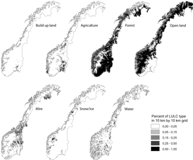
The coverage of the different land use/land cover types is far from uniform, as shown inFig. 1. Built-up and agricultural land are both marginal land use/land cover types in Norway. Built-up land covers only 0.5% of the total area and is highly dispersed. Agriculture covers 3.4% of the area but the pattern is clustered with some areas having a much higher percentage of agriculture, close to 50% around the Oslo fiord. Forest and open land are the two dominant land use/land cover types in Table 1
Descriptive statistics (sum, population mean and population variance) for the seven land use/land cover types in the gridded version of the national land use/land cover map AR50.N¼350,514 grid cells.
Land cover class N Sum (km2) Meanm(km2) Variances2 1 Built-up land 350,514 1859.25 0.00530 0.002105 2 Agriculture 350,514 12,658.59 0.03611 0.013735 3 Forest 350,514 126,113.46 0.35980 0.134033 4 Open land 350,514 140,148.26 0.39984 0.171475 5 Mire 350,514 21,722.85 0.06197 0.016112 6 Snow/ice 350,514 3038.19 0.00867 0.005934 7 Water 350,514 18,559.31 0.05295 0.020069
Norway, covering 35.6% (forest) and 40.4% (open land) of the total area. The“open land”is predominantly heath and does in our study include both coastal and mountain heath. Both forest and open land are found in abundance, exhibiting complementary large scale pattern were areas are covered with either forest or open land. Mire shows a slightly clustered pattern resembling agriculture, but covering a larger area (6.2% of total). Snow/ice is again a small land use/land cover type (0.9% of total) but exhibits a highly clustered pattern (due to the presence of large glaciers) as opposed to the more dispersed built-up land. Water differs from the other land use/ land cover types with an allover more even distribution of mixed size lakes covering altogether 5.3% of the area.
The AR50 map was partitioned into quadratic 1 square kilometer tiles based on the standardized statistical grid for Norway published by Statistics Norway (Strand and Bloch, 2009), resulting in a population consisting ofN¼350,514 regular tiles. By using a GIS overlay function, the acreage of the seven land use/land cover classes was calculated for each tile (grid cell). The result was anN7 matrix of georeferenced land use/land cover observations representing the entire population of tiles.
The population of tiles was subdivided intoK¼100 clusters by randomly choosing a block of 10 by 10 tiles to initiate the partition. Each of the 100 tiles in this block was used as the starting point for one cluster, by including every 10th grid cell in each cardinal direction from the initial tile. Each cluster represents a possible systematic random sample from the population, and the 100 clusters defined by the exercise include all the possible clusters in the population (based on the standard-ized grid and a sampling intensity using 10 km intervals). In order to facilitate computation, column number (c) and row number (r) within the cluster was also assigned to each grid cell.
Since the entire population was known, statistics representing true values could be computed for each of the seven land use/land cover variables (Table 1). The table includes the total area, population mean (m) and variance (s2) for each class. 2.2. Method
The study was conducted in three steps: Thefirst step aimed to demonstrate the efficiency of systematic random sampling compared to simple random sampling;
the second step compared different methods for estimation of the variance of the systematic random sample; and thefinal step examined the influence of spatial structure and distribution on the variance of the different land use/land cover types. The entire population was available in the material for this study, and so was the pseudo-truth consisting of all the 100 clusters representing the possible systematic random samples given the chosen partition. The research questions could therefore be addressed as a model performance characterization exercise (Bennett et al., 2013) with the sampling methods and variance estimation algorithms treated as models and by using the entire population and a complete set of clusters as the modeling environment.
2.2.1. Efficiency of systematic random sampling
Simple and systematic random sampling was examined by comparing the uncertainty resulting from different sampling strategies under otherwise similar conditions and with the same sampling effort. The uncertainty measure selected for the comparison was the variance of the estimatedxfrom samples with equal sample size, thus representing the same sampling effort, but obtained with the two different sampling strategies. Due to the irregular shape of the country, the number of tiles in each of the 100 clusters varied between 3474 and 3538. The mean number of tiles was 3505.14 which was truncated to 3505 and a simple random sample size ofn¼3505 was used as the basis for comparison.
The variance of the estimatorxcomputed from a simple random sample of sizen is
VARðxÞn¼ s2ðNnÞ
nðN1Þ (1)
The expected variance of land cover estimates based on simple random sam-plingVARðxÞncan thus be found by usings2fromTable 1and settingN¼350,514 andn¼3505. The corresponding (exact) variance based on systematic random sampling (VARðxÞSYS) was found by using all the 100 clusters available in the study to determine empirically the distribution of the 100 estimated mean values (bx).
VARðxÞSYS¼1 K XK j¼1 b xjx2 (2) x¼1 N XN i¼1 xi bxj¼1 nj Xnj k¼1 xk
whereKis the number of potential clusters andnjis the number of tiles in clusterj. The varianceVARðxÞSYSwas compared toVARðxÞby applying anFtest where
F¼s21 s2 2
¼ VARðxÞn
VARðxÞSYS (3)
with the expected larger variance placed as the numerator and the degrees of freedom set to 3504 (n1) and 99 (K1). The test is one-sided, because a sys-tematic random sample is expected to have less variance than the equivalent simple random sample. The null-hypothesis (no difference) is rejected if theFvalue is larger than a selected criticalFvalue (hereF0.05,3504,99¼1.29). The result is obviously closely linked to the unit size (tiles) and cluster size (distance between samples), but examination of this variability is not within the scope of the paper. Here, the test is only intended as an indicator of the efficiency of the systematic sampling strategy when the sampling effort isfixed. In our case, the units are 1 km2 grid cells and the sampling effort is approximately 3500 sample units.
2.2.2. Variance estimation methods for systematic random samples
The second research question was concerned withfinding the most appropriate way to estimate the variance from a systematic random sample in the normal sit-uation, when only a single sample is available. Several methods (algorithms) were compared. The algorithms were selected due to the relative ease of implementation and are all applicable in an operational environment. Each method was applied for every land use/land cover class and used for all the 100 clusters in the material, resulting in an empirical approximation of the variation to be expected by that particular method.
The common, but reportedly biased approach is to estimate the variance in a systematic random sample by using the traditional simple random sampling vari-ance estimation method. The grid cells in the cluster are treated as independently and randomly sampled individuals giving a sample size ofn. Notice that the result, VARðxÞSRS, is basically different fromVARðxÞnwhich was used above. WhileVARðxÞn is the variance expected in a true simple random sample,VARðxÞSRSis the estimate of the variance obtained when a systematic random sample is handled as a simple random sample.
The estimate obtained by applying the methodology from simple random sampling is: VARðxÞSRS¼ 1 nðn1Þ Xn i¼1 ðxibxÞ2 (4) wherexiis the amount of a land use/land cover type in tileiandnis the number of grid cells in the cluster andbxis the sample mean.
Several variance estimators based on local differences were evaluated. These estimators use the concept of a“neighborhood”around each sampling unit. This neighborhood is a“sample neighborhood”, not a“population neighborhood”. It consists of a set of 33 units located geographically next to each other in the sample. Thefirst local estimator VARðxÞLO9 was computed using the average local variance for overlapping neighborhoods of 3 by 3 sample tiles:
VARðxÞLO9¼1 n2 Xn i¼1 s2 i (5)
wherenis the total number of tiles in the cluster ands2
iis the variance in the sample neighborhood around tilei:
s2 i ¼ 1 m Xm j¼1 xjxi2 (6)
wherexiis the local mean in the neighborhood around tileiandmis the number of valid data values in the sample neighborhood. This is usually nine in a 3 by 3 tile neighborhood, but may be less if some of the neighbors are missing in the sample (which may be the case along the coastline and the national border).
The second local estimatorVARðxÞLO5 resembledVARðxÞLO9 but was computed excluding the four corner tiles of the 33 sample neighborhood. Thefive remaining tiles were the tile at the center of the neighborhood and the four sample tiles directly east, west, north and south of this tile. The effect of this limited neighbor-hood is that the distance between the tiles in the computation is shorter and the effect of autocorrelation increases.
The third local estimatorVARðxÞST9 was calculated using non-overlapping strata where each stratum is a 3 by 3 tile sample neighborhood. The estimation methods from stratified random sampling were then applied to the sample
VARðxÞST9¼Xk i¼1 w2 i s2 iðNiniÞ niðNi1Þ (7)
wherekis the number of strata,niis the sample size in stratumi(valid cases, mostly nine in our case),s2
iis the variance in stratumi,Niis the population size in stratumi (in our case always set to 100nisince each tile in the sample“represents” 1010¼100 tiles) and:
wi¼ Ni
N (8)
whereNiis the population size in stratumias explained above andNis the total number of tiles in the population.
The fourth local estimatorVARðxÞST4 was similar toVARðxÞST9 but the size of the stratum was limited to four tiles (2 by 2).
The last local estimatorVARðxÞSEMused the geostatistical concept of semi-variance. Each pair of observations in the dataset is separated by a certain dis-tance and can be grouped into a range of disdis-tance intervals, known as lags. The semi-variance for a laghis calculated from the pairs of observations falling into that particular lag as gðhÞ ¼ 1 2m Xm i¼1 ðxixiþhÞ2 (9)
wheremis the number of pairs in laghand each pairiconsist of the observationsxi andxiþh.
VARðxÞSEM¼gðhminÞ=n (10)
wherehminis the distance between the closest observations in the sample (10 km in our case) andnis the number of observations in the sample.
This collection of variance estimation methods for the systematic random sample was compared with the exact variance among the 100 clusters:VARðxÞSYS. The variance estimates were also drawn as box-plots in order to allow visual in-spection assisting the interpretation of the results (Fig. 2).
2.2.3. Spatial structure and distribution of different land use/land cover types The fourth research question was concerned with the impact of spatial structure and distribution of the different land use/land cover types on the variance. Spatial structure is here mainly a question about the influence of spatial autocorrelation and wasfirst approached by calculating Global Moran'sI(Moran, 1950) for distances up to and including the separation between the systematic sampling units (10 km). Computation was carried out followingLegendre and Legendre (1998, p. 715)
GMI¼ 1 W Pn i¼1 Pn j¼1wijðxibxÞ xjbx 1 n Pn i¼1ðxibxÞ2 (11) wherewijis 1 for all pairs included in the computation,Wis the total number of pairs included andbxis the sample mean. Moran'sIreportedly outperforms other tests in simulation experiments (Anselin, 2001) but may, as all global measurements of spatial autocorrelation, be less useful when the basic assumption of stationarity is violated (Anselin, 1995). It should be pointed out that we did not attempt to use GMI as a precise measurement of spatial autocorrelation by e.g. calculating statistical significance. GMI is in this context only used as an indicator.
The assumption, based on existing theory (Cochran, 1977), is that the advantage of systematic sampling is linked to the presence of spatial autocorrelation. TheF -ratio for the land use/land cover classes (described above) was used as an indicator of the advantage of systematic sampling over simple random sampling. TheF-ratio is used here as an index, not a statistic. There is no test of the significance of theF-ratio involved. The purpose is to investigate the assumed relationship between autocor-relation and the advantage of systematic sampling. According to this assumption, theF-ratio will increase as GMI is increasing.
The assumption can be described as an expected presence of a (possibly linear) relationship between theF-ratio and GMI
F¼1:0þc$GMI (12)
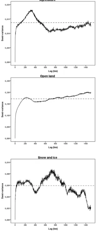
whereFis theF-ratio,GMIis the autocorrelation andcis the impact of autocorre-lation on theF-ratio. The constant (1.0) is the expectedF-ratio when spatial auto-correlation is absent. The relationship was explored graphically using a scattergram. In order to further investigate and be able to discuss the results, we also ob-tained a variogram for each of the land cover classes. The variogram is a curve describing the semi-variance (Equation(9)above) as a function of the lag distance (h). The variogram also illustrates the autocorrelation in the material and shows how the spatial structure is related to distance. A variogram representing a stationary process (where variation depends on distance alone, independent of location) usually shows a smooth curvefirst increasing with distance but thenflattening at a certain level (called the sill) at a particular distance (called the range). The sill represents the population variance and the range can be interpreted as the extent of
the autocorrelation effect. A variogram that does not becomeflat but continues to rise or assumes other shapes is a sign of“drift”in the material. Variation is in this case not only an effect of distance, but also of location.
3. Results
3.1. Proficiency of systematic random sampling
The expected variance of the estimatorxfor the seven land use/
land cover types, computed from a simple random sample of size 3505 and a systematic random sample of approximately the same
size are listed inTable 2. The results of theFtest comparing the two
variance estimates are also listed inTable 2.
The calculatedFvalue is larger than the criticalFvalue (1.29) and
pis therefore smaller than 0.05 for all land cover classes except
built-up land. The variance of the estimator for built-up land is also smaller when systematic random sampling is employed, but the
difference is negligible and not statistically significant. The results
indicate that systematic random sampling, as expected, is more
efficient than simple random sampling for all seven land use/land
cover classes but the improvement is only statistically significant
for six of the seven classes.
3.2. Variance estimation methods for systematic random samples
The empirically determined exact variance of the estimatedx
from systematic random sampling VARðxÞSYS is compared with
each of the proposed estimations of the same variance inTable 3.
Comparison ofTables 2 and 3shows thatVARðxÞSRSreturns a
result slightly higher than, but close to, the variance from a real Fig. 2.Results from the variance estimation methods (SRS,LO9,LO5,STR9,STR4 andSEM) calculated from a population divided into 100 clusters by systematic sampling on a 10 by 10 km frame. Dashed (upper) line shows the variance expected from a simple random sample of the same size. The exact variance for the mean of the 100 systematic samples (VARðxÞSYS) is shown as the dotted (lower) line. Three land use/land cover classes are included, representing the typical patterns.
simple random sample of the same size (VAR(x)3505). This method
also clearly overestimates the variance when systematic random sampling is employed.
All the remaining methods are better alternatives
thanVARðxÞSRS, but none manage to give a correct estimate of the
variance. The results obtained by three of the methods (LOx and
ST9) are fairly similar, and all three are better thanSEM. Among
these,LO5 was consistently better than the other two.ST4 does in
most cases produce results closest to the true variance, but does in some also situations underestimate the variance.
The results can be inspected inFig. 2where the variance
es-timates are shown as box plots. Each plot represents one of the seven land use/land cover types. For each land use/land cover type, the plot shows the empirically determined exact variance for systematic random sampling with the selected sample size as the lower dotted line. The variance expected from a simple random sample of approximately the same size is shown as the upper dashed line. Each of the boxes represents one of the variance estimation methods in the study. The box representing the vari-ance estimated when the sample is treated as a simple random
sample (SRS) is generally the least preferable method (furthest
from the lower dotted line) and (as expected) always close to the variance expected from a true simple random sample (upper dashed line). None of the methods give results systematically
close to the lower dotted line, butST4 is in general returning the
best results.ST4 is also the method with the least scattered results.
The disadvantage regardingST4 is the fact that it falls below the
dotted line for built-up land, showing that the variance in this case is underestimated.
3.3. Spatial structure and distribution of different land use/land cover types
Global Moran'sI(GMI) was used to calculate a spatial
autocor-relation index for all of the seven different land use/land cover types. All variables exhibit some degree of spatial autocorrelation (Table 2). The spatial autocorrelation was particularly high for mire
(0.504) and open land 0.401). The land use/land cover types Forest (0.357), snow/ice (0.340) and agriculture (0.231) revealed a more intermediate spatial autocorrelation, while build-up land (0.050) and water (0.132) returned index values showing relatively small spatial autocorrelation.
TheF-ratio (Table 2) was used as an indicator of the advantage of
systematic sampling over simple random sampling. The
relation-ship between theF-ratio and the spatial autocorrelation is
illus-trated inFig. 3. There is an apparent linear relationship between the
F-ratio and the spatial autocorrelation. Wefitted a reference line
(the dashed line inFig. 3) at
F¼1:0þ5:0$GMI
whereFis theF-ratio (as inTable 2)and GMI is the autocorrelation
(Global Moran'sI). This reference line is indicative of the
relation-ship. The positive effect of systematic sampling, indicated by F, is
increasing steadily as the autocorrelation increases. Fig. 3 does,
however, also show marked deviation from the general rule, in
particular with respect to the category mire where theF-ratio (here
interpreted as the advantage of applying systematic sampling) is considerably less than expected from observation of the spatial autocorrelation.
4. Discussion
In our experiment, two-dimensional systematic sampling per-formed better than simple random sampling for all seven land use/
land cover types. The improvement was statistically significant for
six of the types. This is as expected and only confirms frequently
reported results from other studies (see Introduction). The improvement is closely related to spatial autocorrelation in the material, with highest improvement for the land use/land cover types exhibiting the strongest autocorrelation, which is in
agree-ment with e.g.Payandeh (1970), Dunn and Harrison (1993)and
D'Orazio (2003). The exception is mire where only moderate improvement with systematic sampling notwithstanding the presence of relatively high spatial autocorrelation.
The enhanced accuracy was hidden when the variance was estimated by treating the systematic sample as a simple random sample and neither of the alternative variance estimation methods examined here were able to fully account for the improvement.
VAR(x)ST4, where small local neighborhoods consisting of groups of
four tiles each were treated as non-overlapping strata did in most cases give the best results, but underestimated the variance for built-up land, where spatial autocorrelation is particularly weak.
ST4 is not unique in this respect. All the methods, includingSRS
occasionally underestimate the variance for built-up land.
The analysis of the impact of spatial autocorrelation on theF
-ratio, which was used as an indicator of the advantage of systematic random sampling, showed a detectable and fairly linear
relation-ship between the two variables (Fig. 3). The advantage of
system-atic sampling is increasing with increasing autocorrelation. Mire Table 2
Expected variance from a simple random sample ofn¼3505 (VARðxÞn) and the empirically determined (exact) variance in a systematic random sample of approximately the same size (VARðxÞSYS). Both are transformed from km2(used in Table 1) to % for increased readability. The two variance measurements are compared using anFtest. Global Moran'sI(GMI) is a measure of the spatial auto-correlation in the material.
Land cover class VARðxÞ VARðxÞSYS F p GMI 1 Built-up land 0.0061 0.0050 1.19 0.14 0.049 2 Agriculture 0.0392 0.0213 1.84** 0.01 0.231 3 Forest 0.3824 0.1219 3.14** <0.01 0.357 4 Open land 0.4892 0.1440 3.40** <0.01 0.401 5 Mire 0.0460 0.0186 2.47** <0.01 0.504 6 Snow/ice 0.0169 0.0062 2.75** <0.01 0.340 7 Water 0.0573 0.0341 1.68** <0.01 0.132 Table 3
The empirically determined variance of the estimate from systematic random sampling (SYS) compared to the average value obtained by the proposed estimation methods (SRS,LO9,LO5,ST9,ST4 andSEM). The measurements are transformed from km2(used inTable 1) to % for increased readability. See text for further explanation of each method. Land cover class VARðxÞSYS VARðxÞSRS VARðxÞLO9 VARðxÞLO5 VARðxÞST9 VARðxÞST4 VARðxÞSEM
1 Built-up land 0.0050 0.0066 0.0052 0.0046 0.0057 0.0041 0.0056 2 Agriculture 0.0213 0.0433 0.0301 0.0261 0.0304 0.0235 0.0328 3 Forest 0.1219 0.4054 0.2253 0.1954 0.2213 0.1655 0.2428 4 Open land 0.1440 0.5157 0.2761 0.2390 0.2783 0.2031 0.2944 5 Mire 0.0186 0.0479 0.0334 0.0293 0.0330 0.0251 0.0368 6 Snow/ice 0.0062 0.0185 0.0136 0.0118 0.0127 0.0094 0.0156 7 Water 0.0341 0.0621 0.0524 0.0466 0.0498 0.0394 0.0608
represents and anomaly, since the benefit of systematic sampling is substantially less than expected from the observed autocorrelation. 4.1. Individual land cover classes
Built-up land was the land use/land cover class where the advantage of systematic sampling was smallest (and not
statisti-cally significant). Built-up land is a marginal land use/land cover
class in Norway and also the class with the lowest spatial auto-correlation. Norwegian settlements are small and the unit of
observation in our study is a 1 km2tile. The extent of built-up land
in a tile therefore has only weak predictive strength with respect to the amount of built-up land in the adjacent sample tiles at 10 km
intervals. The variogram (Fig. 4) shows a curve reaching the sill
(representing the population variance and shown as a dotted hor-izontal line in the graph) after approximately 12 km only. The examined variance estimation methods for systematic random sampling (including treating the sample as a simple random sam-ple) all produced fairly identical results for built-up areas, indi-cating that there is little or no advantage from applying systematic sampling in this situation, but also no disadvantage either. There is, however, a risk of underestimating the variance when local esti-mators are used for this class.
Agriculture covers 3.4% of the land in Norway. This land use/ land cover type exhibits stronger autocorrelation than built-up land, probably because agricultural use is closely linked to climate, soil conditions and arability and therefore more
predict-able. As a result, systematic random sampling give significantly
better results than simple random sampling for this class. The
semivariogram (Fig. 4) shows pronounced periodicity. The
func-tion does not stabilize at the sill (dotted line representing the population variance) but climbs to a peak at around 400 km before it falls back below the sill. There is a hint of drift as well, with a small but steady rise in semivariance over increasing distance.
Agriculture deviates from the overall trend inFig. 3, showing that
the effect of applying systematic sampling is less than expected
from the observed spatial autocorrelation. Agriculture does in this sense resemble mire.
The two land use/land cover classes' forest and open land exhibit the most evident spatial autocorrelation in the material,
shown by a noticeable “range” (distance) where the function is
flattening. These are also the two classes where the positive effect
of systematic sampling is highest. We notice that both classes are associated with smooth variograms showing minor periodicity and a slight, probably negligible drift.
Mire has the strongest autocorrelation among the land use/land cover classes studied here, but stand out as markedly different from
the other classes inFig. 3. The variogram (Fig. 4) also show strong
periodicity and does not stabilize at the sill but climbs to a peak at around 500 km before it falls back to the sill. A second peak is found around 1000 km and a pronounced negative drift is observed beyond this distance. This is linked to the regional patterns also
visible inFig. 1where large occurrences of mire are seen in
south-eastern, central and northern Norway. Within these regions, another pattern is visible where Mire frequency change between
valleys and mountains. Mire is mainly found onflat areas found as
valley bottoms, moors and old glacial moraines, but rarely on the steeper slopes separating these locations. The result is a spatial mosaic, although without clearly discernible patterns.
Snow/Ice also has a complex variogram, temporarily reaching the sill after approximately 25 km but showing marked periodicity over longer distance. There is also negative drift in the variogram, similar to the drift exhibited by mire. Permanent snow and ice is a marginal land cover type mainly found as glaciers in mountain areas with high precipitation but the occurrence is massive when the type is present. The advantage of systematic sampling is still pronounced, and higher than for mire.
Thefinal land use/land cover type, water (actually fresh water)
exhibits weak but visible spatial autocorrelation. The advantage of systematic random sampling over simple random sampling is still
clearly present and also statistically significant. Water is found
allover Norway, the spatial pattern is scattered and the spatial Fig. 3.Relationship between the improved accuracy obtained by systematic sampling (F-ratio) and spatial autocorrelation (Global Moran'sI). The reference line is drawn at F¼1.0þ5 GMI.
distribution is fairly random. There are, however, three important differences between built-up land and water: there is more land covered with water than built-up areas (5.3% against 0.5%), water is found more frequently (the class is present in 42% of the tiles) than built-up land (only present in 4% of the tiles) and water is a natural
land cover class, clearly different form the artificial class built-up
land.
Payandeh (1970)found that systematic random sampling per-formed poorly when applied to uniformly spaced forest pop-ulations. This is to some extent contradictory to our result with respect to water. Water is a uniformly spread land use/land cover type in Norway, but we found that systematic random sampling
still was a more efficient sampling method than simple random
sampling (although not necessarily the most efficient).Dunn and
Harrison (1993)found that natural vegetation with complex and varied spatial pattern was related to poor performance of system-atic sampling. This effect was also to some extent observed in our study. Systematic sampling performed best when autocorrelation was present and the process fairly stationary, without periodicity and drift. Examples are in our case forest and open land, but also water where the variogram was smooth and systematic sampling performed well notwithstanding a lesser autocorrelation.
Three classes stand out in our study: Built-up land because systematic sampling had no detectable positive effect due to very small spatial autocorrelation, and agriculture and mire where the
benefit from applying systematic sampling were pronouncedly
lower than expected from the spatial autocorrelation. The latter results may possibly be linked to non-stationarity or periodicity in the material. This could possibly be controlled for by de-trending,
e.g. by applying median polish (Cressie, 1991; Strand, 1998) or by
using a local (instead of a global) autocorrelation statistic (Anselin,
1995).
Among the variance estimation methods tested here, the methods based on local variation all gave more correct variance estimates than when the sample was treated as a simple random sample. The local estimation methods still largely overestimated the variance except for built-up land. This is not necessarily a problem. In applied use with real systematic random samples and no pseudo-truth, it has been argued that variance estimation methods should slightly overestimate the variance to be sure that
the variance is not underestimated (Tomppo and Heikkinen, 1999;
Heikkinen, 2006). The method that gave the best overall results,
VARðxÞST4, systematically underestimated the variance for the least
autocorrelated land type and must therefore be used with great caution.
4.2. Autocorrelation
While our approach to estimation of the variance under sys-tematic sampling is design-based, other studies follow an alter-native geostatistical model-based approach that accounts for
spatial autocorrelation.Aubry and Debouzie (2000)obtained good
results with this approach, but also reported that their method was highly sensitive to the approximation used in the calculation. The experimental variograms for the seven land cover/land use
classes (Fig. 4) show the autocorrelation structure in the material.
Periodicity is present in all seven variograms and some vario-grams also exhibit pronounced drift in the material (seen as a systematic rise or fall toward the right end of the curve). Clearly, none of the land use/land cover classes studied here are associ-ated with simple and smooth variograms with predictable
behavior. It is therefore difficult to use methods relying on an
exact mathematical description of the curves represented by the variograms as required by model-based geostatistical approaches to uncertainty.
Systematic sampling is a design where the entire population is divided into groups (clusters) and one of these clusters is randomly selected as the sample. The total variation in the population has two components: The variation within the clusters and the variation between the clusters. The variance of the mean is the variation between the clusters. Local variation between the adjacent sample units is a coarse measurement of the variation between samples caused by the differences between the origin of each cluster sam-ple. The local variance estimators work because they emphasize this short-distance variation.
The absence of a positive effect from systematic sampling for built-up land and the low effect for agriculture and mire must be caused by a relatively high variation between the clusters. This is normal when spatial autocorrelation is absent and there is little or no difference in variation between and within the clusters. The explanation in the presence of spatial autocorrelation could be linked to systematic patterns on a scale that interfere with the combination of observation units and distance between observa-tions in the selected area frame.
Our study used a sampling scheme withfixed distance of 10 km
between the center of the tiles in the sample and afixed tile size of
1 by 1 km. These choices necessarily influence the effect of
peri-odicity and autocorrelation. This is in agreement with Dunn and
Harrison (1993) who found that the gain using systematic random sampling for different land use/land cover types varied with the sampling intensity. We have, in this study, concentrated on comparing methods under controlled settings but acknowledge the need for further studies of the effect of variable sampling intensities.
5. Conclusion
5.1. Characterizing model performance
Afive step procedure for performance evaluation of models is
suggested byBennett et al. (2013). The key elements are 1)
reas-sessment of the aim, scale and scope; 2) characterization of the data for calibration and testing; 3) visual analysis to gain overview of overall performance; 4) selection of basic performance criteria; and 5) consideration of more advanced methods to handle problems. This is also the procedure followed by our paper, which in this respect is an example of a study of model performance.
The aim, scale and scope of systematic sampling and the related variance indicators is to improve the accuracy of environmental information (relative to simple random sampling) within a reasonable budget and provide variance estimates that reveal the
benefit of the systematic approach. The study demonstrate that
systematic sampling in most cases represent an improvement, and that at least some of the variance indicators provide reasonable information about the uncertainty.
There was no calibration involved and therefore no concern about dependency between the models and the data used for testing. Our test bed was a complete enumeration based on a dataset with national coverage and included seven different land cover classes with variable characteristics, magnitude and spatial distribution. The setting ensures that many aspects of data vari-ability are covered. The shortcoming is that the study was limited to
observation units of afixed size (1 km2) and with afixed sampling
frequency (every 10 unit in both directions). The study could be improved by introducing other sampling unit (grid cell sizes) and sampling frequencies.
Visual analysis was an important tool to gain overview of the overall performance of the models. The main instrument was the box plots that clearly demonstrated the differences between alternative models and for different land cover classes. The box
plots showed the difference between simple random sampling and systematic sampling and simultaneously visualized how the vari-ance indicators behaved in relation to the two sampling methods. We found that the visual analysis was an excellent tool that allowed us to compare and assess models without determining strict formal criteria in advance.
The basic performance criteria for comparing the two sampling methods was the negative (rejection of a null-hypothesis) result of
anF-test of the empirically determined mean variance expected
from each sampling method. The test is easily interpretable and the result clear. Formally, the test could instead have been carried out as a Monte-Carlo simulation using repeated pairs of randomly selected samples (one simple random and one systematic). This
would defuse the possible criticism of anF-test comparingfixed
numbers. The advantage of systematic sampling is, however, already an accepted fact and this part of the performance test can be view as added value rather than as a main objective of the study.
The basic performance criteria for comparing the variance in-dicators were linked to the visual interpretation of the box plots. An acceptable indicator should not underestimate the variance in a systematic sample, i.e. the entire box representing the variation in the outcome of the indicator should be placed above the line rep-resenting the empirically determined variance among the sys-tematic samples. Furthermore, the desirable indicator would be the indicator returning the lowest variance estimate among those
in-dicators acceptable according to thefirst criterion. Finally, if several
indicators performed equally according to thefirst two criteria, the
indicator with the smallest internal variation (most compact box in the box plot) would be preferable.
Finally, alternative methods using geostatistical approaches are acknowledged and referenced in the Introduction as well as in the Discussion. The models tested by us are simple and have the advantage that they easily can be used in operational surveys and
monitoring. Alternatives based on geostatistical (Aubry and
Debouzie, 2000) and non-parametric approaches (Opsomer et al.,
2012) may give more precise results, especially when auxiliary
variables are available. 5.2. Next step
Many factors may affect the results found in this study. As
pointed out byWang et al. (2010) the performance of a spatial
sampling scheme is controlled by the trinity relationship of the target domain, the geographical distribution of the sample and the statistical method that is applied. It is expected that the use of more detailed land use/land cover types can include more rare and scarce classes exhibiting weaker autocorrelation or being more suscepti-ble to periodicity. This could reduce the advantage of employing
systematic random samples, and the benefit of using local variance
estimation method will be smaller. Furthermore, although
sys-tematic sampling in most cases is shown to be more efficient than
simple random sampling, it is not necessarily the most efficient
sampling strategy. Other approaches, including different forms of
stratification, could be as efficient and also carry the benefit of an
unbiased variance estimation method. The methods and software
described byWang et al. (2013)could be used to examine these
questions in depth.
Our study examined a selection of variance estimation methods for two-dimensional systematic samples. The list is not exhaustive and alternative methods may give an estimate closer to the pseudo-truth. We also notice that local estimation methods work well in most circumstances but underestimate the variance in certain sit-uations. The modeling environment with a complete enumeration allows us to describe these situations. Better methods to assess the
appropriateness of local estimators in a real situation when only a single sample is known will be needed. These questions all warrant further studies.
Our study has demonstrated an advantage of systematic random sampling over simple random sampling and linked the improvement to spatial autocorrelation. The study has also shown that local estimators of variance are superior to variance estimated as if the sample was a simple random sample when systematic random sampling is employed and spatial autocorrelation is
pre-sent. Between the local estimators of variance, stratification into
non-overlapping neighborhoods using the smallest possible strata (2 by 2 tiles) was in most cases the best method, although prone to underestimate the variance when the autocorrelation was small. Until contrary results or better estimators are available, we therefore recommend the use of systematic random sampling coupled with the local estimator of variance using 2 by 2 tile
stratification when spatial autocorrelation is present. The SRS
estimator is a safe alternative in the absence of spatial relation, or when the order of magnitude of the spatial autocor-relation is unknown.
References
Ambrosio, L., Iglesias, L., Marín, C., Del Monte, J.P., 2004. Evaluation of sampling methods and assessment of the sample size to estimate the weed seedbank in soil, taking into account spatial variability. Weed Research 44, 224e236. Anselin, L., 2001. Spatial econometrics. In: Baltagi, B.H. (Ed.), A Companion to
Theoretical Econometrics. Blackwell Publishing, Malden, pp. 310e330. Anselin, L., 1995. Local indicators of spatial associationeLISA. Geographical
Anal-ysis 27, 93e155.
Aubry, P., Debouzie, D., 2000. Geostatistical estimation variance for the spatial mean in two-dimensional systematic sampling. Ecology 81, 543e553.
Axelsson, A.-L., Ståhl, G., Sønderberg, U., Petersson, H., Fridman, J., Lundbstrøm, A., 2010. Sweden. In: Tomppo, E., Gschwanter, T., Lawrence, M., McRoberts, R. (Eds.), National Forest Inventories, Pathways for Common Reporting. Springer, pp. 541e554.
Bellhouse, D.R., Sutradhar, B.C., 1988. Variance estimation for systematic sampling when autocorrelation is present. The Statistician 37, 327e332.
Bennett, N.D., Barry, F.W.C., Guariso, G., Guillaume, J.H.A., Hamilton, S.H., Jakeman, A.J., Marsili-Libelli, S., Newham, L.T.H., Norton, J.P., Perrin, C., Pierce, S.A., Robson, B., Seppelt, R., Voinov, A.A., Fath, B.D., Andreassioan, V., 2013. Characterising performance of environmental models. Environmental Modelling&Software 40, 1e20.
Cochran, W.G., 1977. Sampling Techniques, third ed. John Wiley&Sons, New York. Cressie, N.A.C., 1991. Statistics for Spatial Data. John Wiley&Sons, New York. D'Orazio, M., 2003. Estimating the variance of the sample mean in two-dimensional
systematic sampling. Journal of Agricultural, Biological, and Environmental Statistics 8, 280e295.
Dramstad, W.E., Fjellstad, W.J., Strand, G.H., Mathiesen, H.F., Engan, G., Stokland, J.N., 2002. Development and implementation of the Norwegian monitoring pro-gramme for agricultural landscapes. Journal of Environmental Management 64, 49e63.
Dunn, R., Harrison, A.R., 1993. Two-dimensional systematic sampling of land use. Applied statistics 42, 585e601.
Eurostat, 2003. The Lucas Survey. European Statisticians Monitor Territory. Office for Official Publications of the European Communities, Eurostat, Luxembourg. FAO, 2010. Global Forest Resources Assessment 2010, Main report, Food and
Agri-culture Organization of the United Nations, Rome.
Fattorini, L., Marcheselli, M., Pisani, C., 2006. A three-phase sampling strategy for large-scale multiresource forest inventories. Journal of Agricultural, Biological, and Environmental Statistics 11, 296e316.
Fewster, R.M., Buckland, S.T., Burnham, K.P., Borchers, D.L., Jupp, P.E., Laake, J.L., Thomas, L., 2009. Estimating the encounter rate variance in distance sampling. Biometrics 65, 225e236.
Flores, L.A., Martinez, L.I., Ferrerm, C.M., 2003. Systematic sample design for the estimation of spatial means. Econometrics 14, 45e61.
Gallego, J., Delince, J., 2010. The European land use and cover area-frame statistical survey. In: Benedetti, R., Bee, M., Espa, G., Piersimoni, F. (Eds.), Agricultural Survey Methods. John Wiley&Sons, Chichester, pp. 149e168.
Gautschi, W., 1957. Some remarks on systematic sampling. Annals of Mathematical Statistics 28, 385e394.
Heikkinen, J., 2006. Assessment of uncertainty in spatially systematic sampling. In: Kangas, A., Maltamo, M. (Eds.), Forest Inventory. Methodology and Applications, 10. Springer, Dordrecht, pp. 155e176.
Koop, J.C., 1971. On splitting a systematic sample for variance estimation. Annals of Mathematical Statistics 42, 1084e1087.
Legendre, P., 1993. Spatial autocorrelation: trouble or new paradigm? Ecology 74, 1659e1673.
Legendre, P., Legendre, L., 1998. Numerical Ecology, second English edition. Elsevier, Amsterdam.
Madow, W.G., Madow, L.H., 1944. On the theory of systematic sampling, I. The Annals of Mathematical Statistics 15, 1e24.
Martino, L., Fritz, M., 2008. New Insight into Land Cover and Land Use in Europe. Land Use/cover Area Frame Statistical Survey: Methodology and Tools. Statistics in focus 33. Eurostat, Luxemburg.
Matern, B., 1947. Methods of Estimation the Accuracy of Line and Sample Plot Surveys. Meddelanden från Statens Skogforskningsinstitutt 36.
Matern, B., 1960. Spatial variation. Stochastic models and their application to some problems in forest surveys and other sampling investigations. Meddelanden fran Statens Skogs- forskningsinstitut 49, 1e155.
Milne, A., 1959. The centric systematic area-sample treated as a random sample. Biometrics 15, 270e297.
Moran, P.A.P., 1950. Notes on continuous stochastic phenomena. Biometrika 37, 17e23. Opsomer, J.D., Francisco-Fernandez, M., Li, X., 2012. Model-based non-parametric variance estimation for systematic sampling. Scandinavian Journal of Statis-tics 39, 528e542.
Payandeh, B., 1970. Relative efficiency of two-dimensional systematic sampling. Forest Science 16, 271e276.
Stehman, S.V., 2009. Sampling designs for accuracy assessment of land cover. In-ternational Journal of Remote Sensing 30, 5243e5272.
Strand, G.-H., 1998. Large-scale variations in radial tree growth in Norway: an application of median polish for spatial trend detection. Applied Geography 18, 153e168.
Strand, G.-H., 2013. The Norwegian area frame survey of land cover and outfield land resources. Norsk Geografisk TidsskrifteNorwegian Journal of Geography 67, 24e35.
Strand, G.-H., Bloch, V.V.H., 2009. Statistical Grids for Norway. Documentation of National Grids for Analysis and Visualization of Spatial Data in Norway. Sta-tistics Norway, Oslo.
Ståhl, G., Allard, A., Esseen, P.-A., Glimsk€ar, A., Ringvall, A., Svensson, J., Sundquist, S., Christensen, P., Torell, Å., H€ogstrom, M., Lagerqvist, K., Marklund, L., Nilsson, B.,€ Inghe, O., 2011. National inventory of landscapes in Sweden (NILS)escope, design, and experiences from establishing a multiscale biodiversity monitoring system. Environmental Monitoring and Assessment 173, 579e595.
S€arndal, C.E., Swensson, B., Wretman, J., 2003. Model Assisted Survey Sampling. Springer, New York.
Thompson, S.K., 2002. Sampling, second ed. John Wiley&Sons, New York. Tomppo, E., Heikkinen, J., 1999. National forest inventory of Finlandepast, present
and future. In: Alho, J. (Ed.), Statistics, Registries, and Science. Experiences from Finland. Statistics Finland, Helsinki, pp. 89e108.
Tomppo, E., Tuomainen, T., 2010. Finland. In: Tomppo, E., Gschwanter, T., Lawrence, M., McRoberts, R. (Eds.), National Forest Inventories, Pathways for Common Reporting. Springer, pp. 185e206.
Tomter, S.M., Hylen, G., Nilsen, J.E., 2010. Norway. In: Tomppo, E., Gschwanter, T., Lawrence, M., McRoberts, R. (Eds.), National Forest Inventories, Pathways for Common Reporting. Springer, pp. 411e424.
Verburg, P.H., Neumann, K., Nol, L., 2011. Challenges in using land use and land cover data for global change studies. Global Change Biology 17, 974e989. Wang, J.-F., Haining, R., Cao, Z.D., 2010. Sample surveying to estimate the mean of a
heterogeneous surface: reducing the error variance through zoning. Interna-tional Journal of Geographic Information Science 24, 523e543.
Wang, J.-F., Stein, A., Gao, B.-B., Ge, Y., 2012. A review of spatial sampling. Spatial Statistics 2, 1e14.
Wang, J.-F., Jiang, C.-S., Hu, M.-G., Cao, Z.-D., Guo, Y.-S., Li, L.-F., Liu, T.-J., Meng, B., 2013. Design-based spatial sampling: theory and implementation. Environ-mental Modelling&Software 40, 280e288.
Wolter, K.M., 1984. An investigation of some estimators of variance for systematic sampling. Journal of American Statistical Association 79, 781e790.
Wolter, K.M., 2007. Introduction to Variance Estimation, second ed. Springer, New York.
Wu, C.F.J., 1984. Estimation in systematic sampling with supplementary observa-tions. Sankhya: The Indian Journal of Statistics, Series B (1960e2002) 46, 306e315.
Wyatt, B.K., 2000. Vegetation mapping from ground, air and spaceecompetitive or complementary techniques? In: Alexander, R., Millington, A.C. (Eds.), Vegetation Mapping: from Patch to Planet. John Wiley&Sons, Chichester, pp. 3e15.
Zinger, A., 1980. Variance estimation in partially systematic sampling. Journal of the American Statistical Association 75, 206e211.