Fractionally integrated processes and structural changes: theoretical analyses and bootstrap methods

OpenBU http://open.bu.edu

Theses & Dissertations Boston University Theses & Dissertations

2014

Fractionally integrated processes

and structural changes: theoretical

analyses and bootstrap methods

GRADUATE SCHOOL OF ARTS AND SCIENCES

Dissertation

FRACTIONALLY INTEGRATED PROCESSES AND STRUCTURAL CHANGES: THEORETICAL ANALYSES AND BOOTSTRAP

METHODS

by

SEONG YEON CHANG

B.A., Seoul National University, 2002 B.S., Seoul National University, 2002

M.A., State University of New York - Albany, 2008

Submitted in partial fulfillment of the requirements for the degree of

Doctor of Philosophy 2014

First Reader

Pierre Perron, PhD Professor of Economics

Second Reader

Zhongjun Qu, PhD

Associate Professor of Economics

Third Reader

Hiroaki Kaido, PhD

I would like to express my sincere gratitude to my advisor, Professor Pierre Perron for his guidance and patience. He has been supportive and understanding at all times. I should admit that I can complete my dissertation through his invaluable encouragement.

I also wish to thank Professor Zhongjun Qu for constructive discussion and advice on my research. Moreover, I am indebted to Professor Iv´an Fern´andez-Val and Hiroaki Kaido for their teaching and advising me.

Lastly, my heartfelt appreciation goes to my family. To my parents, I am thankful for your love and your countless sacrifice. To my lovely wife, Yangshin Park, I am very pleased to share this moment with you. I always thank you for being with me. To my precious son, Matthew, you have been my bliss and inspiration in my journey.

CHANGES: THEORETICAL ANALYSES AND BOOTSTRAP METHODS

(Order No. )

SEONG YEON CHANG

Boston University, Graduate School of Arts and Sciences, 2014 Major Professor: Pierre Perron, Professor of Economics

ABSTRACT

The first chapter considers the asymptotic validity of bootstrap methods in a linear trend model with a change in slope at an unknown time. Perron and Zhu (2005) analyzed the consistency, rate of convergence, and limiting distributions of the parameter estimates in this model. I provide theoretical results for the asymptotic validity of bootstrap methods related to forming confidence intervals for the break date. I consider two bootstrap schemes, the residual (for white noise errors) and the sieve bootstrap (for correlated errors). Simulation experiments confirm that confidence intervals obtained using bootstrap methods perform well in terms of exact coverage rate.

The second chapter extends Perron and Zhu’s (2005) analysis to cover more general fractionally integrated errors with memory parameter d in the interval (−0.5,1.5). My theoretical results uncover some interesting features. For example, with a concurrent level shift allowed, the rate of convergence of the estimate of the break date is the same for all values of din the interval (−0.5,0.5), a feature linked to the contamination induced by allowing a level shift. In all other cases, the rate of convergence is decreasing as dincreases. I also provide results about the spurious break issue.

The third chapter considers constructing confidence intervals for the break date in linear regressions. I compare the performance of various procedures in terms of the exact coverage rates and lengths: Bai’s (1997) based on the asymptotic distribution with shrinking shifts,

of the change, Eo and Morley’s (2013) based on inverting a likelihood ratio test, and various bootstrap procedures. In terms of coverage rates, EM’s approach is the best but with a high cost in terms of length. With serially correlated errors and a change in intercept or in the coefficient of a regressor with a high signal-to-noise ratio, or when a lagged dependent variable is present, the length approaches the whole sample as the magnitude of the change increases. This drawback is not present for the other methods. Theoretical results are provided to explain the drawbacks of EM’s method.

1 Asymptotic Validity of Bootstrap Methods for a Structural Break in

Trend 1

1.1 Introduction . . . 1

1.2 The Model and Key Inequality . . . 4

1.3 The Case withi.i.d. Errors . . . 7

1.3.1 Residual Bootstrap . . . 8

1.3.2 Functional Central Limit Theorem for Residual Bootstrap . . . 9

1.3.3 Higher-order Refinements . . . 13

1.4 The Case with Serially Correlated Errors . . . 15

1.4.1 Sieve Bootstrap . . . 15

1.4.2 Higher-order Refinements . . . 20

1.5 Monte Carlo Experiments . . . 21

1.6 Empirical Application . . . 26

1.7 Conclusion . . . 28

1.8 Appendix . . . 29

2 Inference on a Structural Break in Trend with Fractionally Integrated Errors (with Pierre Perron) 61 2.1 Introduction . . . 61

2.2 Fractionally Integrated Processes and Functional Central Limit Theorem . . 64

2.3 The Models and Assumptions . . . 66

2.3.1 A Key Inequality . . . 69

2.4.1 Consistency . . . 70

2.4.2 Rate of Convergence . . . 72

2.4.3 The Limiting Distribution of the Estimate of the Break Date . . . . 73

2.4.4 The Limiting Distribution of Other Parameters . . . 76

2.5 Spurious Break . . . 78

2.6 Simulation Experiments . . . 82

2.6.1 Finite Sample and Limiting Distributions . . . 82

2.6.2 Spurious Break . . . 86

2.7 Conclusion . . . 87

2.8 Appendix . . . 88

2.8.1 Results for Model I . . . 88

2.8.2 Results for Model II . . . 103

3 A Comparison of Alternative Methods to Construct Confidence Intervals for the Estimate of a Break Date in Linear Regression Models (with Pierre Perron) 126 3.1 Introduction . . . 126

3.2 The Model and Procedures . . . 130

3.2.1 Bai’s (1997) Approach . . . 130

3.2.2 Elliott and M¨uller’s (2007) Approach . . . 133

3.2.3 Bootstrap Methods . . . 134

3.2.4 Likelihood-based Method . . . 138

3.3 Simulation Experiments . . . 140

3.4 Theoretical Results about Elliott and M¨uller’s (2007) Approach . . . 143

3.4.1 Static Regression with Serially Correlated Errors . . . 143

3.4.2 Dynamic Regression . . . 146

3.5 Conclusion . . . 149

Bibliography 160

Curriculum Vitae 168

1.1 i.i.d. errors . . . 41

1.2 AR(1) errors . . . 41

1.3 ARMA(1,1) errors . . . 42

1.4 (Log) Nominal Exchange Rates with respect to the US dollars . . . 43

1.1 i.i.d. error, T = 200 . . . 44 1.2 i.i.d. error, T = 800 . . . 45 1.3 AR(1) error, φ1 = 0,T = 200 . . . 46 1.4 AR(1) error, φ1 = 0,T = 800 . . . 47 1.5 AR(1) error, φ1 = 0.3,T = 200 . . . 48 1.6 AR(1) error, φ1 = 0.3,T = 800 . . . 49 1.7 AR(1) error, φ1 = 0.5,T = 200 . . . 50 1.8 AR(1) error, φ1 = 0.5,T = 800 . . . 51 1.9 AR(1) error, φ1 = 0.8,T = 200 . . . 52 1.10 AR(1) error,φ1 = 0.8,T = 800 . . . 53 1.11 ARMA(1,1) error,φ1 = 0.8, ψ=−0.3,T = 200 . . . 54 1.12 ARMA(1,1) error,φ1 = 0.8, ψ=−0.3,T = 800 . . . 55 1.13 ARMA(1,1) error,φ1 = 0.8, ψ=−0.5,T = 200 . . . 56 1.14 ARMA(1,1) error,φ1 = 0.8, ψ=−0.5,T = 800 . . . 57 1.15 ARMA(1,1) error,φ1 = 0.8, ψ=−0.9,T = 200 . . . 58 1.16 ARMA(1,1) error,φ1 = 0.8, ψ=−0.9,T = 800 . . . 59

1.17 (Log) Nominal Exchange Rates to the US dollars [−: Break date, −−: BP, − · −: SM] . . . 60

2.1 Finite sample and asymptotic distribution in Model I and II with d∗= 0.2: µ0_b = 0. . . 120

2.2 Finite sample and asymptotic distribution in Model I and II with d∗= 1.2: µ0_b = 0. . . 121

2.4 Finite sample and asymptotic distributions in Model II with d = 0.2 and

µ0_b 6= 0. . . 123 2.5 Finite sample and asymptotic distributions in Model II with d∗ = 1.2 and

µ0

b 6= 0. . . 124 2.6 Empirical Distribution of ˆT1 when there is no change in trend . . . 125

3.1 Coverage Rate and Average Length of Confidence Intervals . . . 157 3.2 Power Functions of ˆUT([T λ]) in Dynamic Regression Models (T = 100, λ0 = 0.5)158 3.3 Limits of ˆUT([T λ]) in Dynamic Regression Models (T = 100, λ0 = 0.5) . . . 159 3.4 Limits of ˆUT([T λ]) in Dynamic Regression Models (λ0 = 0.5, λ= 0.3) . . . . 159

AIC . . . Akaike Information Criterion AR . . . Autoregressive

ARFIMA Autoregressive Fractionally Integrated Moving Average ARMA . . Autoregressive Moving Average

BIC . . . Bayesian Information Criterion

BP . . . Bootstrap Percentile (PB in Chapter 3) BT . . . Bootstrapt

CDF . . . . Cumulative Distribution Function CIs . . . Confidence Intervals

DGP . . . . Data Generating Process EM . . . Elliott and M¨uller (2007)

i.i.d. . . Independent and Identically Distributed ILR . . . Inverting the Likelihood Ratio test LM . . . Lagrange Multiplier

LR . . . Likelihood Ratio MA . . . Moving Average

OLS . . . Ordinary Least Squares PZ . . . Perron and Zhu (2005) SM . . . Standard Method

SSR . . . Sum of Squared Residuals

Asymptotic Validity of Bootstrap Methods for a

Structural Break in Trend

1.1 Introduction

In the econometrics and statistics literature, testing for a structural break and estimating the break date have been popular topics (see Perron, 2006, for a review). Since Perron’s (1989) work, it is well known that structural breaks play important roles in the statistical

inference of economic time series.

For the structural break in a linear time trend, the following work are relevant. Chu and White (1992) consider a test for a change in trend with stationary errors. Perron (1991) and Vogelsang (1997) analyze testing procedures for a slope change in trend when the errors are either stationary or have a unit root. Vogelsang (1999) devises a test whose limiting distribution does not change depending on whether the noise component is stationary or integrated. Recently, Perron and Yabu (2009) consider testing for a structural change in the trend function of a time series without any prior knowledge about whether the errors are stationary or integrated. Their testing procedure adopts a quasi-feasible generalized least squares (GLS) approach that uses a super-efficient estimate of the sum of the autoregressive parametersα whenα= 1. Harveyet al. (2009) propose a GLS-based trend break test that is asymptotically size robust with I(0) and I(1) errors.

When testing results imply that there is a structural change in trend, we want to perform inference about the change date. In order to construct confidence intervals (CIs), of

interest is the limiting distribution of the estimate of the break date. As an important early treatment, Hinkley (1970) considers a sequence of i.i.d. random variables. Feder (1975) deals with segmented regressions that are continuous at the break date. Bhattacharya (1987) analyzes the maximum likelihood estimates in a multi-parameter case. However, the limiting distribution derived in those studies depends on the exact distributions of the regressors and the errors. Since the exact distributions are unknown a priori, it makes statistical inference difficult. To avoid this problem, a framework with shrinking shifts is adopted in the literature.

In the shrinking shifts framework, the magnitude of a change is assumed to be decreasing as the sample size increases. The rate of decrease, however, is not so fast to allow estimating the break fraction consistently. In the econometrics literature, Bai (1997) considers both fixed and shrinking break in a linear regression model. Although the limiting distribution is non-standard, the quantiles of interest can be obtained numerically (see Bai, 1997, appendix B). Bai and Perron (1998) generalize the assumptions on the regressors and the errors and consider regression models with multiple structural breaks. Stock and Watson (2002) analyze an AR(1) model with a structural break for various economic variables and apply Bai’s (1997) method for constructing confidence intervals. They claim that 95% confidence intervals are so wide as to be uninformative, so that they decide to report 67% confidence intervals.

Confidence intervals are frequently used in conjunction with point estimates to convey information about the uncertainty of the estimate. In contrast to the large literature on dating the break date, work pertaining to forming accurate confidence intervals for the break date is more scarce. Bai and Perron (2006) provide extensive simulation experiment results and report the coverage rates of confidence intervals constructed by the standard method of Bai (1997). Elliott and M¨uller (2007) claim that this standard method cannot be a good choice for constructing confidence intervals when the magnitude of a break is small. They suggest a test that is locally invariant to the magnitude of break in linear regression models. Confidence sets are obtained by inverting the test. More recently, Eo and Morley (2013)

generalize Siegmund’s (1988) likelihood ratio test to a system of multivariate equations. Confidence sets are also constructed by inverting the likelihood ratio test. Chang and Perron (2013a) compare the performance of various procedures in terms of exact coverage rate and average length of the confidence intervals, they also show that the test of Elliott and M¨uller (2007) has a non-monotonic power function when either the errors are serially correlated or a lagged dependent variable is introduced as a regressor in the model. In such cases, the length of the confidence interval approaches the whole sample as the magnitude of the break increases.

The most relevant work related to this paper is Perron and Zhu (2005) (PZ, henceforth). They analyze consistency, rate of convergence, and limiting distribution of parameter estimates in models where the trend function exhibits a slope change at an unknown time with or without a concurrent change in level. They consider the dichotomous cases whereby the errors are stationary or have a unit root. Chang and Perron (2013b) extend PZ’s work to fractionally integrated processes. In the present paper, we consider the so-called joint broken trend model defined below.

I find some interesting theoretical results. Let λ0 ∈(0,1) denote the true break fraction. ˆ

λis the estimate of the break fraction in a sample and ˆλ∗ is the bootstrap correspondent of ˆ

λ. First, I can prove the asymptotic validity of bootstrap methods. Based on the theoretical derivations in PZ, I can show that the bootstrapped statistic T3/2(ˆλ∗−λˆ) conditionally weakly converges to the limiting distribution of T3/2(ˆλ−λ0) in probability. It means that both the bootstrapped statistic and the sample statistic have the same limiting distribution. Second, I show that bootstrap methods have higher order refinement. Bootstrap percentile and bootstrapt confidence intervals are considered and simulation experiments show that those bootstrap-based confidence intervals have good finite sample properties in terms of the exact coverage rate compared to the confidence intervals obtained from the standard method.

The structure of this paper is as follows. In section 2, I present the model and a key inequality that will be used repeatedly. In section 3, I first consider the case in which

the error is a sequence of i.i.d. random variables. I review residual bootstrap and the invariance principle pertaining to residual bootstrap. The consistency, rate of convergence, and limiting distribution of the bootstrapped statistic are presented and higher order refinement is achievable with residual bootstrap. In section 4, the errors are allowed to be a stationary process, in which case the sieve bootstrap is adopted. Based on the invariance principle for the sieve bootstrap, I show its asymptotic validity. Furthermore, we show that higher order refinement is also possible with seive bootstrap. In section 5, finite sample experiments are performed in order to support the theoretical results. In section 6, I analyze the (log) nominal exchange rates with respect to the US dollars for eight countries. The break dates and the 95% bootstrap percentile confidence intervals are provided. Section 7 provides brief concluding remarks and an appendix contains all theoretical derivations.

1.2 The Model and Key Inequality

A univariate time seriesyt is assumed to be the sum of a systematic part ft and a random component ut, that is, for t= 1,2, . . . , T,

yt=ft+ut. (1.1)

For ut, we assume Eut = 0. For the systematic part ft, we assume that it contains a first-order linear trend with a one time change in slope such that the trend function is joined at the time of break. We call it as joint broken trend model. This corresponds to Model I(b) in PZ. The break date is denoted by k∈_Nand we define the break fraction as

λ=k/T.

The deterministic component ft is specified by

where Bt is the dummy variable for a slope change defined by Bt=      0 ift≤k, t−k ift > k

with a candidate break date k. By introducing a dummy variable Bt, we assume that the slope coefficient changes fromβ toβ+δ at datek. In matrix notation, the model is specified as follows

Y =Xkγ+U (1.3)

where Y = (y1, . . . , yT)0, U = (u1, . . . , uT)0, Xk = (x(k)1, . . . , x(k)T)0 where x(k)0t = (1, t, Bt), and γ = (µ, β, δ)0. Note that the matrix Xk depends on the postulated value of the break datek. The parameters are estimated using a global least-squares criterion. Precisely, the break date is estimated as follows

ˆ

k= arg min k

Y0(I−Pk)Y (1.4)

where Pk is the projection matrix on the space spanned by Xk, i.e. Pk=Xk(Xk0Xk)−1Xk0. Let X_kˆ be constructed using the estimate of the break date ˆk. The OLS estimate of γ is then ˆ γ = (X_ˆ0 kXˆk) −1_X0 ˆ kY (1.5)

and the resulting sum of squared residuals is, for an estimated break fraction ˆλ= ˆk/T,

S(ˆλ) = T X t=1 ˆ u2_t = T X t=1 yt−x(ˆk)0tγˆ 2 =Y0(I−Pˆ_k)Y (1.6)

where P_kˆ is the projection matrix associated with Xˆ_k.

The true values of unknown parameters will be denoted with a 0 subscript, i.e.,γ0, k0, λ0;

Xk0 is the matrix of regressors constructed using the true valuek0 for the break date, and

Y =Xk0γ0+U. PZ show that plimT→∞λˆ=λ0. When the error is a stationary process, the rate of convergence is ˆλ−λ0 =Op(T−3/2) (Theorem 3 in PZ), and the limiting distribution of the estimated break fraction is given by

T3/2(ˆλ−λ0)⇒N 0, 4σ 2 λ0(1−λ0)δ2 (1.7)

where σ2 is a finite variance of the error ut and ⇒ denotes weak convergence under the Skorohod topology (see Theorem 4 in PZ).

Let U∗ denote a vector of resampled regression residual ˆut based on some bootstrap schemes. Then, we can construct new process {y_t∗}, and in matrix notation,

Y∗ =Xˆ_kγˆ+U∗ (1.8)

where U∗= (u∗₁, . . . , u∗_T)0. Similar to (1.4), we can estimate the break date ˆk∗ from (1.8). Accordingly, the bootstrap estimate of the break fraction is denoted ˆλ∗ = ˆk∗/T.

Here, we need to check an important inequality that plays a crucial role in proving asymptotic properties. Note that the estimate of the break date ˆkis treated as a true break date in the bootstrap sample. By construction, for allT, in a bootstrap sample

S(ˆλ∗)≤S(ˆλ)

or equivalently,

Y∗0(I−Pˆ_k∗)Y

∗ _≤

Y∗0(I−Pˆ_k)Y∗.

Since Y∗ =X_kˆγˆ+U∗, the inequality can be rewritten as

or equivalently, (ˆγ0X_ˆk0 +U∗0)(Pˆ_k−P_kˆ∗)(Xˆ_kγˆ+U∗) = ˆγ0X_ˆ0 k(Pˆk−Pkˆ∗)X_kˆγˆ+ 2ˆγ0X_kˆ0(P_kˆ−P_kˆ∗)U∗+U∗ 0 (Pˆ_k−Pˆ_k∗)U∗ = ˆγ0(Xˆ_k−Xˆ_k∗) 0 (I−Pˆ_k∗)(X_kˆ−Xˆ_k∗)ˆγ+ 2ˆγ 0 (X_kˆ−Xˆ_k∗) 0 (I−Pˆ_k∗)U ∗ +U∗0(P_kˆ−P_kˆ∗)U ∗ = (XX) + 2(XU) + (U U)≤0. (1.9) Note that X_ˆ0 kPˆk=X 0 ˆ k and X 0 ˆ

k(I−Pkˆ) = 0 in the second equality. Moreover, we know that

arg min k S(k) = arg min k [S(k)−S(ˆk)] = arg min k [ˆγ0(Xˆ_k−Xˆ_k∗)0(I−Pˆ_k∗)(Xˆ_k−Xˆ_k∗)ˆγ + 2ˆγ0(X_kˆ−Xˆ_k∗)0(I−Pˆ_k∗)U∗+U∗ 0 (P_kˆ−P_kˆ∗)U∗]. (1.10)

We will use this equation to derive the asymptotic distribution of the bootstrap estimate of the break fraction, ˆλ∗.

The aim is to show the asymptotic validity of the bootstrap distribution of ˆλ∗−λˆ. We derive the limiting distribution of T3/2(ˆλ∗−λˆ) and show that it is equivalent to that of

T3/2(ˆλ−λ0) in probability. Because Freedman (1981) considers the limiting distribution of regression coefficients and showsT1/2-consistency under some regularity conditions, we focus on the estimate of the break date in the present paper.

1.3 The Case with i.i.d. Errors

As a benchmark, we consider a joint broken trend model with i.i.d. errors. The data generating process is specified as

where δ6= 0. For ut, we assume that the following assumption holds.

• Assumption 1: {ut} is a sequence of i.i.d. random variables with mean zero and finite variance σ2. Moreover, T−1/2P[T r]

t=1ut ⇒ σW(r), r ∈ [0,1] where [·] is the greatest smaller integer function andW(·) is the standard Wiener process.

1.3.1 Residual Bootstrap

Freedman (1981) introduces the concept of the residual bootstrap in regression models where the regressors are not stochastic and the errors are i.i.d. with mean zero and finite variance. We review the residual bootstrap in the joint broken trend model briefly.

At first, we estimate the model by the ordinary least square (OLS) method and obtain the OLS residual {uˆt}, that is,

ˆ ut=yt−µˆ−βtˆ −δBˆ t, t= 1,2, . . . , T where Bt=      0 ift <kˆ t−kˆ ift≥k.ˆ

Note that the dummy variableBtis associated with the estimate of the break date ˆk. We can define the empirical cumulative distribution function of {uˆt} by

F∗(z) =T−1

T

X

t=1

1ˆut≤z

and resample, for any t∈_Z,u∗_t from F∗. Then we construct {y∗_t} as follows:

y_t∗= ˆµ+ ˆβt+ ˆδBt+u∗t, t= 1,2, . . . , T.

For each bootstrap sample, we can estimate the date of the structural break ˆk_b∗ with

1.3.2 Functional Central Limit Theorem for Residual Bootstrap

We need to introduce some notations for the bootstrap procedure. Let P∗ denote the probability measure conditional on data and errors{xt, ut} so that

P∗kˆ∗−kˆ ≤z =Pkˆ∗−ˆk ≤z|{x_t, u_t}T_t=1 .

Similarly, E∗,Var∗, and Cov∗ are defined conditional on{xt, ut}.

Remark 1. For the following proofs in Appendix, we need to introduce the symbolso∗_p and

O_p∗ for the bootstrap sample asymptotics, which correspond to op and Op for the original

sample asymptotics. We follow the definitions in Chang and Park (2003). Let {X_N∗} be a sequence of bootstrapped statistics. Define X_N∗ =o∗_p(1)a.s. (in P) to imply that for all

>0,

P∗(|X_N∗|> )→0 a.s.(inP)

as N → ∞, respectively. Moreover, if for every >0, there exists a constant M and an

integer N such that

P∗(|X_N∗|> M)< for allN ≥N,

we write X_N∗ = O∗_p(1) a.s. or in P depending on whether the condition holds a.s. (with probability one), or holds in P (with probability arbitrarily close to one). It is easy to show that if E∗|X_N∗| → 0 a.s. (or in P), then X_N∗ = o∗_p(1) a.s. (or in P). Similarly, if

E∗|X_N∗|=O(1)a.s. (or in P, i.e., Op(1)), then X_N∗ =Op∗(1)a.s. (or in P).

Remark 2. For a sequence of bootstrapped statistics {X_N∗}, we write

X_N∗ →d∗ X a.s.(in P) (1.12)

if the conditional distribution of{X_N∗}weakly converges to that ofX a.s.(or inP). We can show that X_N∗ =O∗_p(1)a.s. (or in P) if a sequence of bootstrapped statistics {X_N∗} weakly convergesa.s.(or inP). When the distribution ofXis degenerate, we writeX_N∗ →p∗ X a.s.

(or in P).

Antochet al. (1995) show the asymptotic validity of the residual bootstrap for a change in mean model. The model is defined as

yt=      θ+t t= 1, . . . , k0, θ+δ+t t=k0+ 1, . . . , T,

where δ6= 0 andtis ani.i.d. random variable with zero mean and finite varianceσ2. With some regularity conditions and a shrinking shift framework, they prove the following results.

sup z∈_R P∗(ˆδ2(ˆk∗−kˆ)≤z)−P(δ2(ˆk−k₀)≤z) →0 a.s., sup z∈R P∗(ˆδ2(ˆk∗−ˆk)/σ∗2 ≤z)−P(δ2(ˆk−k0)/σˆ2≤z) →0 a.s..

This result implies that the bootstrap distribution can be a good approximation to the exact distribution asymptotically. Huˇskov´a and Kirch (2008) consider a change in mean model when the errors are stationary and strong mixing. They prove the asymptotic validity of a circular moving block bootstrap as suggested by Politis and Romano (1992) to deal with stationary process.

Remark 3. A shrinking shift framework is pervasive in the literature related to structural changes. In this framework, the magnitude of a change is assumed to be decreasing as the sample size increases, but the rate of shrinkage is not so fast that the break fraction can be estimated consistently. If the size of a change is fixed, the limiting distribution of the estimate of the break date depends on the exact distributions of the regressors and the errors. Given that the exact distributions of the regressors and the errors are unknown a priori in general, we often rely on a shrinking shift framework to avoid this problem. Although the limiting distribution is non-standard even with a shrinking shift, we can obtain the quantiles of interest numerically (see, e.g., Bai, 1997).

joint broken trend model with stationary errors, PZ derive the limiting distribution of the estimate of the break fraction without a shrinking shift framework, surprisingly the limiting distribution is Normal. This result sheds a light on the validity of bootstrap methods. Since the limiting distribution of the estimate of the break fraction is Normal in a joint broken trend model, we can establish the asymptotic validity of bootstrap methods by showing that the bootstrap statistic(ˆλ∗−ˆλ)T3/2 _{has the same asymptotic distribution as the corresponding}

sample statistic (ˆλ−λ0)T3/2.

In order to establish the validity of the bootstrap, I show that the limiting distribution of the bootstrap statistic is the same as that of the sample statistic. The invariance principle is the key element for that purpose. For each resampling{u∗_t}of the OLS residuals{uˆt}∞t=1, we define W_T∗(r) = 1 ˆ σ√T [T r] X t=1 u∗_t, r∈[0,1] (1.13)

which is the bootstrap counterpart for WT(r) = (σ

√

T)−1P[T r]

t=1ut, where ˆσ2 =E∗(u∗t2) =

T−1PT

t=1uˆ2t. The invariance principle for bootstrap states that

W_T∗ →d∗W a.s.(inP). (1.14)

Basawaet al. (1991) prove the invariance principle (1.14) under the assumptionE(u2_t)<∞. They show (1.14) by proving that the finite dimensional distributions converge in the Mallows metric and that the tightness condition holds. Ferretti and Romo (1996) prove (1.14) in the space C[0,1] of real continuous functions on [0,1]. They also prove the weak convergence of finite dimensional distributions and tightness with the supremum norm. The invariance principle in Park (2002) is of strong form, which holds almost surely for all realizations. Here, we review the results in Park (2002) for completeness. The Donsker’s theorem says thatWT →dW in the space D[0,1] of c´adl´ag functions. The space D[0,1] is equipped with the uniform normk · k in the sequel. The Skorohod representation theorem shows that there exists a probability space (Ω,F,P) supporting a process W_T0 that has

the same distribution as WT and such thatW_T0 →a.s.W. Sakhanenko (1980) derives the so-called strong approximation, which proves the existence ofW_T0 satisfying the following condition.

Lemma 1.3.1 (Strong approximation). Let E|ut|r <∞ for somer >2. Then we have for

anyη >0

P{kW_T0 −Wk ≥η} ≤T1−r/2κrE|ut|r,

where κr is an absolute constant depending only on r.

Because WT and WT0 have the same distribution, we can assume that WT →a.s. W uniformly if we are only interested in distributional results. Now, consider the partial sum (1.13) again. By Lemma 3.1, we can find a W_T∗0 such that

P{kW_T∗0−W∗k ≥δ} ≤T1−r/2κrE∗|u∗t|r. (1.15)

W_T∗0 has the same distribution as W_T∗ in an extended probability space rich enough to support a standard Brownian motionW∗, so that we do not distinguish W_T∗0 fromW_T∗. The following lemma is straightforward from (1.15).

Lemma 1.3.2 (Theorem 2.2 in Park, 2002). If E∗|u∗_t|r_{<∞ a.s. and}

T1−r/2E∗|u∗_t|r →_a.s.0 (1.16)

for some r >2, then

W_T∗→d∗W a.s.

as T → ∞.

If condition (2.1) is satisfied, then W_T∗ →_p∗ W∗ almost surely because of the strong

approximation (1.15). It is easy to show that W_T∗ →_d∗ W∗. As Park (2002) noted, W_T∗ →d∗ W a.s. since the distribution of the limit process W∗ is independent of the

Theorem 1.3.1 (Consistency). Under Assumption 1, if condition (2.1)holds, thenλˆ∗ →p∗

ˆ

λalmost surely.

Theorem 1.3.2 (Rate of Convergence). Under Assumption 1, if condition (2.1) holds,

thenλˆ∗−λˆ=O∗_p(T−3/2) almost surely.

Theorem 1.3.3 (Limiting Distribution). Under Assumption 1, if condition (2.1) holds, then T3/2(ˆλ∗−λˆ)→_d∗N 0, 4σ 2 λ0(1−λ0)δ2 inP.

Theorem 3.3 implies that the bootstrap statistic T3/2(ˆλ∗−ˆλ) has the same asymptotic distribution as the corresponding sample statisticT3/2(ˆλ−λ0) in probability. Therefore, it establishes the asymptotic validity of the bootstrap distribution.

1.3.3 Higher-order Refinements

The Edgeworth expansion provides another perspective on the bootstrap method for constructing confidence intervals for the break date. We consider the Edgeworth expansions of both the standardized estimator (ˆλ−λ0)(Σ/

√

T)−1 where Σ−1=δpk0(T−k0)(2σ)−1 and the studentized estimator (ˆλ−λ0)( ˆΣ/

√

T)−1 where ˆΣ−1 = ˆδ

q

ˆ

k(T−ˆk)(2ˆσ)−1. Define Rt= (ytx(k)t0, vec(x(k)tx(k)t0)0)0 and ν =E(Rt) = (Γ0Qxx, vec(Qxx)0)0. We can rewrite (ˆλ−λ0)(Σ/

√

T)−1 in the form of √T A( ¯R) where ¯R = PT

t=1Rt, and A(ν) = 0. Since this expansion has been established exactly in Bhattacharya and Ghosh (1988) and Hall (1986), we only state the result without proof.

Theorem 1.3.4. Suppose that δ 6= 0, λ0 ∈ (0,1), and two additional conditions hold:

(i) E(kRtk3) < ∞ and (ii) lim supktk→∞|E[exp(it0Rt)]| <1, where i=

√

−1. Then, the standardize estimator (ˆλ−λ0)(Σ/

√

T)−1 and its bootstrap counterpart (ˆλ∗−ˆλ)( ˆΣ/√T)−1 admit the following Edgeworth expansion uniformly overz almost surely:

P λˆ−λ0 Σ/√T ≤z|F ! = Φ(z) +p(√z|F) T φ(z) +o(T −1/2_{), (1.17)}

P λˆ ∗_−λˆ ˆ Σ/√T ≤z| ˆ F ! = Φ(z) +p ∗_(z|Fˆ) √ T φ(z) +o(T −1/2_{). (1.18)}

Moreover, p(z|F) is a polynomial of degree 2 with coefficients depending on λ0,Γ and

moments ofRt up to order 3. p∗(z|Fˆ)is the bootstrap counterpart ofp(z|F)with coefficients

depending on ˆλ,Γˆ and moments of R∗_t.

Theorem 1.3.5. Suppose that δ 6= 0, λ0 ∈ (0,1), and two additional conditions hold:

(i) E(kRtk3) < ∞ and (ii) lim supktk→∞|E[exp(it0Rt)]| <1, where i=

√

−1. Then, the studentized estimator (ˆλ−λ0)( ˆΣ/

√

T)−1 and the bootstrap counterpart (ˆλ∗−λˆ)( ˆΣ∗/√T)−1 admit the following Edgeworth expansion uniformly overz almost surely:

P λˆ−λ0 ˆ Σ/√T ≤z|F ! = Φ(z) +q(√z|F) T φ(z) +o(T −1/2_{), (1.19)} P ˆλ ∗_−λˆ ˆ Σ∗/√T ≤z| ˆ F ! = Φ(z) +q ∗_(z|Fˆ) √ T φ(z) +o(T −1/2_{). (1.20)}

q(z|F) is a polynomial of degree 2 with coefficients depending on λ0,Γ and moments of Rt

up to order 3. q∗(z|Fˆ) is the bootstrap counterpart of q(z|F) with coefficients depending on ˆ

λ,Γˆ and moments of R∗_t.

These theorems are informative for evaluating the accuracy of the bootstrap and asymptotic distributions as approximations to the exact distribution of (ˆλ−λ0)( ˆΣ/

√ T)−1. Since Σ is not feasible, we are interested in the studentized estimator. The expansions (1.19) and (1.20) yield P ˆ λ−λ0 ˆ Σ/√T ≤z|F ! −P ˆ λ∗−ˆλ ˆ Σ∗_/√_T ≤z|Fˆ ! =T−1/2[q(z|F)−q∗(z|Fˆ)]φ(z) +o(T−1/2) (1.21) almost surely. The first term in (1.21) has size O(T−1) almost surely uniformly over z. Now the bootstrap makes an error of size O(T−1_{), which is smaller as T → ∞ than the} error made by the first order approximation O(T−1/2). This result comes from the fact that q(z|F)−q∗(z|Fˆ) =O(T−1/2) and ˆk,Γ and the moments ofˆ R∗_t approachk0,Γ and the

moments ofRtat rate T−1/2.

1.4 The Case with Serially Correlated Errors

1.4.1 Sieve Bootstrap

B¨uhlmann (1997) introduces the sieve bootstrap for dependent data. To use the sieve bootstrap, the time series of interest is approximated by a finite order autoregressive process. The order is an increasing function of sample size. The bootstrap samples are obtained from the centered fitted residuals and then new process is constructed by the recursion. If we know the structure of the error process, a parametric bootstrap is available and shows good finite sample properties. However, the structure of the noise component is unknown in general, which motivates one to use the sieve bootstrap.

The DGP is specified as

yt=ft+ut (1.22)

where ft is a systematic part and{ut} are generated as

ut= Ψ(L)t (1.23)

where Lis the usual lag operator, Ψ(z) =P∞

k=0ψkzk, andt is an i.i.d.random variable with E(t) = 0. By Wold’s theorem, a one-sided infinite order MA representation (1.23) is available if ut is a real-valued, stationary process with expectation E(ut) =µu, and purely stochastic, i.e. not deterministic (see, e.g., Brockwell and Davis, 1991). We can rewrite ut as a one-sided infinite-order autoregressive process assuming the process to be invertible,

t= Φ(L)ut (1.24)

where Φ(z) =P∞

moving average processut by a finite order autoregressive process, i.e.,

ut=φ1,Tut−1+. . .+φp,Tut−p+t. (1.25)

Remark 5. A practical issue is how to choose the order p in the autoregression. Two

information criteria are possible. First, the Akaike Information Criterion (AIC) leads to an asymptotically efficient choice for the optimal order of AR(∞) process (see Shibata, 1980). Second, the Bayesian Information Criterion (BIC) has an optimality property when the order of the true underlying autoregressive process is finite. We use the AIC in this paper because the true model is unknown in general and not of finite dimension.

Remark 6. Choi and Hall (2000) provide a set of simulation studies to compare the

performance of the sieve and block bootstrap methods for constructing confidence intervals in both linear and non-linear problems, for example, the sample mean and median are included. They confirm that the choice of the autoregressive order (p) has little effect on the performance in terms coverage accuracy. This property is promising because the block bootstrap is sensitive to the choice of the block length. Furthermore, the confidence intervals formed by the sieve bootstrap show better exact coverage rates than those from the block bootstrap.

Let φ= (φ1,T, . . . , φp,T)0. We can estimate φby OLS or the Yule-Walker equations. In the literature, it is well known that the estimate from the Yule-Walker equations is preferred because they always yield an autoregression that is invertible. It is defined by

Γpφ=γp

and

σ2 =γ(0)−φ0γp

where Γp = [γ(i−j)]p_i,j=1 and γp= (γ(1), . . . , γ(p))0. Based on the Yule-Walker equations, we can estimate ˆφand ˆσ2 from ˆγ(1), . . . ,ˆγ(p). The estimated covariances ˆγ(s) are defined

by ˆ γ(s) =T−1 T X t=s+1 ˆ utuˆt−s.

In addition, we introduce some assumptions for the sieve bootstrap method.

• Assumption 2ut=P∞j=0ψjt−j,ψ0 = 1 (t∈Z) with{t}t∈Zi.i.d.random variables

such thatEt= 0, E2t =σ2,E|t|r<∞for some r >4.

• Assumption 3Letψ(z)6= 0 for all |z| ≤1, andP∞

j=0|j|s|ψj|<∞for somes≥1.

• Assumption 4 Let p = pT → ∞ and pT = o((T /logT)1/2) as T → ∞ and ˆφp = ( ˆφ1,T, . . . ,φˆp,T)0 satisfies the empirical Yule-Walker equations

ˆ

Γpφˆp = ˆγp

where ˆΓp = [ˆγ(i−j)]pi,j=1 and ˆγp= (ˆγ(1), . . . ,ˆγ(p))0.

Under Assumptions 2-3 along with Wold’s theorem, we can consider general linear processes. Assumption 4 is compatible with the use of the AIC to determine the order p in the autoregression.

Lemma 1.4.1. Suppose that Assumptions 2-4 hold with s∈N. Then, as T → ∞,

max 1≤j≤p| ˆ φj−φj|=O((log(T)/T)1/2) a.s., (1.26) sup j∈_N |ψˆj−ψj|=O((log(T)/T)1/2) +O(p−s) a.s., (1.27) ˆ σ2 =σ2+O((log(T)/T)1/2) +o(p−s) a.s. (1.28) ˆ ψT(1) =ψ(1) +O(s(log(T)/T)1/2) +o(p−s) a.s. (1.29)

Lemma 4.1 is a collection of the results derived in Hannan and Kavalieris (1986) and B¨uhlmann (1995), hence I omitted the proof.

We review how to implement the sieve bootstrap. After estimating the parameters of the model, we approximate theM A(∞) process ˆut by a finite order AR(pT) process based

on the AIC. We can then obtain the estimated residuals as ˆ t,T = pT X j=0 ˆ φj,Tuˆt−j

where ˆφ0,T = 1. We center the estimated residuals to set the sample mean zero, i.e.,

˜ t,T = ˆt,T −(T −pT)−1 T X t=pT+1 ˆ t,T (1.30)

and denote the empirical CDF of {˜t,T}Tt=pT+1 by

F∗(z) = (T −pT)−1 T

X

t=pT+1

1˜t,T≤z. (1.31)

We can resample, for anyt∈Z,∗t i.i.d. from F∗, and define{u∗t} by the recursion, pT X j=0 ˆ φj,Tu∗t−j = ∗ t (1.32)

with approximately chosenpT-initial values ofu∗t. To that effect, we set the initial values to zero and construct theAR(pT) process from (3.12) for a sufficiently long period to ensure stationarity of the process. We then discard the initial values to have a sample of size

T+pT. Then, we obtainyt∗ as follows;

y∗_t = ˆµ+ ˆβt+ ˆδBt+u∗t (1.33)

where Bt is associated with ˆk. Similar to thei.i.d. case in the previous section, let

W_T∗(s) = 1 ˆ σT √ T [T s] X k=1 ∗_k (1.34)

be the bootstrap correspondence of the processWT.

(2.1) is satisfied andW_T∗ →_d∗ W almost surely as T → ∞.

The Beveridge-Nelson’s (1981) representation allows a decomposition of utsuch that

ut=ψ(1)t+ (˜t−1−˜t), (1.35)

where ˜t=P∞j=0ψ˜jt−j with ˜ψj =P∞i=j+1ψi. Under Assumptions 2-3, we have

P∞

j=0|ψ˜k|<∞ (see, e.g., Phillips and Solo, 1992, p 973), then the time series{˜t}is well defined in botha.s. and L1 sense.

Let VT(r) = T−1/2P[T r]t=1ut = σψ(1)P[T r]t=1t+T−1/2(˜0 −˜[T r]). We can derive the invariance principle for ut, that is, VT(r)→dV =σψ(1)W(r) from the continuous mapping theorem because max1≤t≤T|T−1/2˜t| →p 0 under Assumption 2-3 (see Phillips and Solo, 1992, p 978).

Of interest is the bootstrap invariance principle for u∗_t. If we let ˆψ(1) = 1/φˆ(1) and

˜ ∗_t = 1 ˆ φ(1) pT X j=1   pT X i=j ˆ φi,T  u∗_t−j+1,

then using the Beveridge-Nelson decomposition again, we have

V_T∗(s) = √1 T [T s] X t=1 u∗_t = (ˆσTψˆ(1)) [T s] X t=1 ∗_t +T−1/2(˜∗₀−˜∗_{[T s]}). (1.36)

Given that ˆσ2_T →a.s.σ2 and ˆψT(1) →a.s. ψ(1) as T → ∞, we would show the invariance principle for{u∗_t} if the following condition holds

P∗ max 1≤t≤T|T −1/2_˜∗ t|> δ →a.s.0 (1.37) for any δ >0.

(2.2) holds and

V_T∗ →_d∗ V =σψ(1)W a.s.

as T → ∞.

Theorem 1.4.1. Under Assumption 2-4,

T3/2(ˆλ∗−ˆλ)→_d∗ N 0, 4ω 2 λ0(1−λ0)δ2 inP as T → ∞ where ω2 =σ2ψ(1)2.

The limiting distribution ofT3/2_(ˆλ∗_{−λˆ) is not asymptotically pivotal. It depends on the} parametersδ, σ2, andψ(1). Further, a consistent estimate of the long run variance is needed in order to use the studentized statistic (ˆλ−λ0)( ˆΣ/

√

T)−1where ˆΣ−1= ˆδ

q

ˆ

k(T−ˆk)(2ˆω)−1. The finite sample performance of the bootstrap confidence intervals will depend on the estimate of the long run variance.

1.4.2 Higher-order Refinements

Choi and Hall (2000) derive the Edgeworth expansion related to the sieve bootstrap. The following assumptions are required to derive the Edgeworth expansion: (a) all moments of the distribution ofu0 are finite, (b) there exists ζ ∈(0,1) such that |φi|+|ψi|=O(ζi) asi→ ∞, (c) the distribution ofu0 is absolutely continuous with a bounded probability density. The implications in the assumptions are referred to Choi and Hall (2000).

Theorem 1.4.2. Suppose thatδ 6= 0, λ0∈(0,1), and assumption (a)-(c) hold. Then, the

standardized estimator (ˆλ−λ0)(Σ/

√

T)−1 and the bootstrap counterpart (ˆλ∗−λˆ)( ˆΣ/√T)−1 admit the following Edgeworth expansion uniformly overz almost surely:

P λˆ−λ0 Σ/√T ≤z|F ! = Φ(z) +ps√(z|F) T φ(z) +o(T −1/2_{), (1.38)} P λˆ ∗_−λˆ ˆ Σ/√T ≤z| ˆ F ! = Φ(z) +p ∗ s_√(z|Fˆ) T φ(z) +o(T −1/2_{). (1.39)}

Moreover, ps(z|F) is a polynomial of degree 2 with coefficients depending on λ0,Γ and

moments ofRtup to order 3. p∗s(z|Fˆ)is the bootstrap counterpart ofps(z|F)with coefficients

depending on ˆλ,Γˆ and moments of R∗_t.

This theorem implies that sieve bootstrap has higher-order refinement. By combining this result with the fact that sieve bootstrap is not sensitive to the choice of the autoregression order p, the sieve bootstrap has substantial advantages over blocking methods when the error is a general stationary process. The proof of this theorem is a direct extension of Choi and Hall (2000), hence it is omitted.

1.5 Monte Carlo Experiments

In this section, we compare the performance of the standard and bootstrap methods in terms of the exact coverage rate and the average length of the confidence intervals. Throughout the simulation experiments, the data-generating process is defined as:

yt=µ+βt+δBt+ut (1.40)

where µ= 1.72,β = 0.03,δ=−0.02, and λ0 = 0.5. Simulations are performed 3,000 times and the bootstrap samples are replicated 4,999 times for each simulation. We consider the following models.

• M1: i.i.d. error;ut∼i.i.d.N(0, σ2) withσ2 = 0.1

• M2: AR(1) error; ut=φ1ut−1+t, φ1 ∈ {0,0.3,0.5,0.8}, andt∼i.i.d.N(0, σ2) with

σ2_{= 0.1}

• M3: ARMA(1,1) error;ut=φ1ut−1+ψt−1+t,φ1 = 0.8,ψ ∈ {−0.3,−0.5,−0.9}, and t∼i.i.d.N(0, σ2) withσ2= 0.1

We compare three different ways of constructing confidence intervals. One is based on the limiting distribution and the others are from the bootstrap distribution.

Standard Method To construct confidence intervals, we need to obtain the quantiles of interest from the limiting distribution. PZ derive the limiting distribution of the estimate of the break date, and it is given in (1.7), that is,

T3/2(ˆλ−λ0)⇒N 0, 4ω 2 λ0(1−λ0)δ2 .

With consistent estimates, we can construct a confidence interval for the break date as

SM ≡ ˆ k−1.96 2 √ Tωˆ q ˆ k(T−kˆ)|δˆ| ,ˆk+ 1.96 2 √ Tωˆ q ˆ k(T−kˆ)|δˆ| . (1.41)

Here, ω2 is simply the variance of the error ut for the model M1, i.e. ω2=σ2, but it is the so-called long-run variance for M2 and M3. To estimate the long-run varianceω2, we adopt an AR(1) approximation forut in Andrews (1991) so that the data-dependent rule for the bandwidth is such that m = 1.1447(C(δ)T)1/θ where C(δ) = 4 ˆφ1(δ)2/(1−φˆ1(δ)2)2 with

ˆ

φ1(δ) the OLS estimate from a regression of ˆut on ˆut−1. We use the quadratic kernel in the simulation experiments, so thatθ= 5. For the Bartlett kernel,θ= 3.

Bootstrap Percentile Confidence Intervals Bootstrap percentile (BP) confidence

intervals are intuitive by construction and easy to implement, so that they are popular in empirical applications. Two types of bootstrap percentile confidence intervals are available. First, we sort the estimated break dates ˆk_b∗, b= 1, . . . , B for sufficiently large B. In doing so, the estimate ˆkshould be included in the sorted set. Then, the quantiles of interest, for example, the 0.025 and 0.975 quantiles, are denoted byK_α/2∗ andK₁∗_−α/2, respectively. The 100(1−α)% bootstrap percentile confidence interval BP_(I) is defined as

BP(I)=

Second, we want to use the fact that ˆk−k0 is well approximated by ˆk∗−ˆk. Let ˆq denote the quantile function for ˆk−k0. Then,

P r ˆ qα/2 ≤kˆ−k0≤qˆ1−α/2 =P r −qˆ1−α/2+ ˆk≤k0≤ −qˆα/2+ ˆk = 1−α.

Here, we use the bootstrapped quantile values K_α/2∗ −ˆk, K₁∗_−α/2 −kˆ in order to replace ˆ

qα/2,qˆ1−α/2, respectively. The 100(1−α)% bootstrap confidence intervalBP(II) is defined as

BP(II)=

2ˆk−K₁∗_−α/2,2ˆk−K_α/2∗ .

Bootstrap t Confidence Intervals Bootstrap t(BT) confidence intervals are defined

as follows. LettT = (ˆk−k0)/ωˆ where ˆω is the standard error of ˆk, and let t∗n= (ˆk∗−ˆk)/ωˆ∗. As usual, denote Hboot(z) =P∗(t∗n≤z) for somez. The two-sided 100(1−α)% bootstrapt confidence interval is defined by

BT = ˆ k−H_boot−1 1−α 2 ˆ ω,kˆ−H_boot−1 α 2 ˆ ω .

In order to use the sieve bootstrap with stationary errors (M2 and M3), we approximate an infinite order moving average process by a fixed order autoregressive process. Then the long-run variance can be estimated by a parametric method. That is, we have anAR(p) processut defined as

(1−φ1L−φ2L2− · · · −φpLp)ut= Φ(L)ut=t,

where t is ani.i.d. random variable with mean zero and finite variance σ2. The autore-gressive parameters are estimated by the Yule-Walker equations and let ˆφ(L) denote the estimated polynomial. Hence, the long-run variance ω2 _{is estimated by}

ˆ

ω2 = σˆ 2 ˆ Φ(1)2,

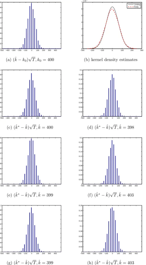
where ˆΦ(1) is the sum of all pcoefficients in the polynomial ˆΦ(L). Figure 1.1-1.16 show histograms for (ˆk−k0)

√

T in panel (a) and the empirical finite sample probability density function (pdf) against the limiting pdf for the estimates of the break date in panel (b). For each model, two sample sizes are considered (T = 200,800). The limiting distribution of (ˆk−k0)

√

T is given in (1.7). To obtain the finite sample pdf, we use the 3,000 simulated statistics and construct an empirical pdf using a non-parametric kernel density estimator.1 The histograms for the bootstrap counterpart (ˆk∗ −ˆk)√T

are in panel (c)-(h). The bootstrap samples are constructed to estimate the break date ˆ

k∗_b, b= 1, . . . ,4999 in each simulation.

In Figure 1.1-1.2, the results withi.i.d.errors are presented. It is true that the asymptotic distribution is a good approximation to the finite sample pdf as the sample size increases. Two interesting features are found. First, the histogram of (ˆk−k0)

√

T and the histograms of the bootstrap counterpart (ˆk∗−ˆk)√T have similar distribution in terms the shape and spread. This feature is more clearer with large sample (T = 800). Hence, the confidence intervals constructed by the bootstrap methods can provide useful improvement. Second, the spreads and shapes of the bootstrap distributions vary a bit but not a lot, so we can rely on the results from the bootstrap methods. Table 1.1 reports the exact coverage rates and the average lengths of the 95% confidence intervals. When the sample size is small (T = 200), the confidence interval formed by the standard method has the exact coverage rate 0.90 that is below the nominal rate 0.95. On the other hand, the bootstrap-based confidence intervals perform better in terms of exact coverage rates even with small samples. Since the limiting distribution is a good approximation withT = 800, the exact coverage rate of the standard method is also close to the nominal rate.

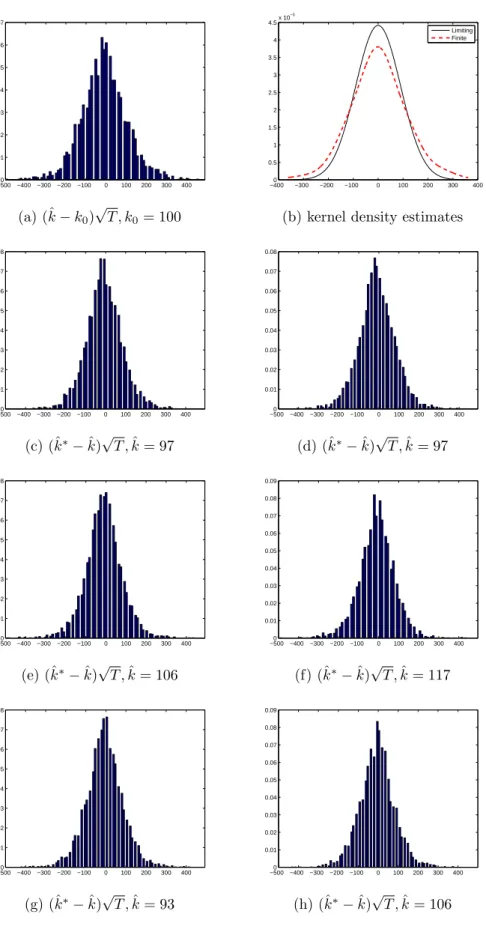
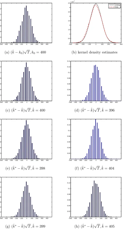
Figure 1.3-1.10 and Table 1.2 report the results pertaining to M2. In figures, the histograms and pdfs are plotted for different values of autoregressive coefficientφ1. First, I

1

For a given set of statistics{Zi}i=1,...,N, the pdf at valuezis estimated byg(z) = (N hz)−1PN_i=1K((z−

Zi)/hz) whereK(·) is the kernel function andhz is the bandwidth. In this paper,N= 3,000 and Gaussian

kernel is used. As mentioned in PZ, the cross-validation method for choosing the optimal bandwidth does not work well here because the estimates of the break date are discrete integers. As a rule of thumb, we set

consider the caseφ1 = 0, that is, the error is a sequence ofi.i.d.random variables, but the sieve bootstrap is applied to form confidence intervals. As expected, the exact coverage rates are less than those with the residual bootstrap but still close to the nominal rate. Next, when anAR(1) process is less persistent, for example, the autoregressive coefficient

φ1∈ {0.3,0.5}, the bootstrap-based confidence intervals perform well in term exact coverage rates. Whenφ1= 0.3, the bootstrap-based CIs have the exact coverage rates around 0.92, which is better than the exact coverage rate 0.84 obtained from the standard method. With φ1 = 0.5, the exact coverage rates are below the nominal rate 0.95. However, the bootstrap-based methods have the exact coverage rates around 0.90 that clearly dominate the standard method having the exact coverage rate 0.77. In Figure 1.9-1.10, the error is assumed to be a persistentAR(1) process with φ1 = 0.8. When the sample size is small, the shapes and spreads of the bootstrap distributions are different from those of the sample distribution. In addition, the limiting distribution cannot be a good approximation to the sample distribution (see Figure 1.9 (b)). As the sample size increases, this problem is alleviated. We find again that the bootstrap distribution provides a closer approximation to the finite sample distribution. When the sample size is T = 200, confidence intervals formed by the standard method have the shortest average length, but the exact coverage rates are far below the nominal rate 0.95. On the other hand, the bootstrap-based methods show better performance in terms of the exact coverage rates and the average length of CIs although the exact coverage rates are also below the nominal rate. With T = 800, the bootstrap-based methods allow the exact coverage rates to be around the nominal rate (φ1 = 0.5) or be conservative sometimes (φ1 = 0,0.3) while the standard method still provides the exact coverage rate 0.91 that is a bit lower than the nominal rate 0.95. Interestingly,BP_(I) marginally dominatesBP_(II) in terms of the exact coverage rates.

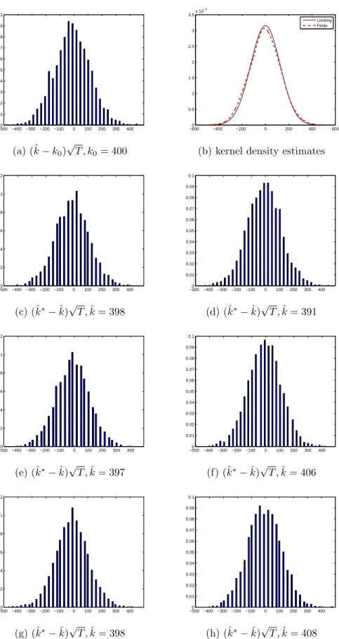
Figure 1.11-1.16 and Table 1.3 report the results related to M3. We assume that the noise component is an ARMA(1,1) process, i.e., (1−φ1L)ut= (1 +ψL)t with φ1 = 0.8. When the moving average coefficient is−0.3, the shape and spread of the sample distribution are different from those of the bootstrap distributions. This disparity is less severe as

the sample size increases or/and the moving average coefficient ψis close to −1. Except for the case with ψ= −0.9, the coverage rates are far below the nominal rate when the sample size isT = 200. WithT = 800, the sieve bootstrap shows better performance than the standard method in terms exact coverage rates. Since the noise component is rather persistent (φ1= 0.8), it has an effect on the precision of the estimation of the break date. It, hence, makes the confidence intervals less accurate even with wider ranges. As the moving average coefficient gets closer to−1, the finite sample performances are improved across all methods.

1.6 Empirical Application

In this section, we examine the nominal exchange rates with respect to the US dollars for eight countries: Australia, Brazil, Canada, China, Japan, Mexico, Singapore and Thailand. The data are obtained from Datastream (2013). All series are analyzed with a logarithm transformation. The results are reported in Table 1.4 and Figure 1.17. Before estimating the break date, it is necessary to test whether there is a slope change in trend function. Recently, Perron and Yabu (2009) suggest a testing procedure for a slope change in trend. The test statistic is based on a quasi-feasible GLS procedure with a super-efficient estimate of the sum of the AR parameterαwhenα= 1. Since this test has nearly the same asymptotic size with both the I(0) andI(1) errors, it is very useful in empirical analysis. Test statistic is reported in the column ”WRQF”. Test results confirm that there exists a structural change in the trend function for all countries considered. The break dates are estimated based on the global least square criterion as in (1.4). As shown in PZ, the estimate of the break fraction is consistent with both the I(0) andI(1) errors. Lastly, unit root test is required for the nominal exchange rate series. If there exists a unit root, we cannot use the sieve bootstrap that is appropriate for a stationary process. Kim and Perron (2009) consider unit root tests allowing a change in slope under both the null and alternative hypotheses. The unit root test first detrends{yt} using the deterministic componentft associated with

the estimate of the break fraction ˆλand then tests the unit root null hypothesis using the

t-statistic on the sum of the autoregressive coefficientsα in the following regression model where {y˜t} denotes the detrended series: for a joint broken trend model,

˜ yt= ˆαy˜t−1+ l X j=1 ˆ dj∆˜yt−j+ ˆut.

Let tpα(ˆλAO1 ) denote the t-statistic in the unit root test. The autoregression order (l) is determined by either the Akaike Information Criterion (AIC) or Bayesian Information Criterion (BIC). For Mexico, the test tpα(ˆλAO1 ) leads to a rejection of the unit root at the 1% significance level. For Australia, Canada, China, Singapore and Thailand, the unit root null hypothesis is rejected at the 5% significance level. For Brazil and Japan, we can reject the null hypothesis at 10% significance level. The critical values for the joint broken trend model are available in Perron and Vogelsang (1993). The sieve bootstrap is used to form the 95% bootstrap percentile confidence interval (BP CI) for the true break date. If the confidence intervals are so wide, they would be uninformative. The lengths of the confidence interval relative to the sample size (reported in the column ”Portion”) are between 0.04 and 0.32.

In empirical analysis, we can use the sieve bootstrap because the unit root test shows that the error is a stationary process. However, if the error is either a long memory process or has a unit root, then we have to make the bootstrap scheme compatible with the structure of the error. As explained above, Kim and Perron (2009) consider unit root tests allowing a change in slope under both the null and alternative hypotheses. Chang (2013) suggests the Lagrange Multiplier tests for a fractional unit root where a structural change is also allowed under both the null and alternative hypotheses. It would be recommended for researchers to test a unit root and/or a fractional unit root as a pre-test. The choice of the bootstrap scheme will depend on the pre-test result.

1.7 Conclusion

In this paper, we show the asymptotic validity of bootstrap methods for a joint broken trend model. In econometrics, bootstrap methods have been popular because of their good finite sample properties along with the advance of high-performance computing capacity. On the other hand, it is also true that the bootstrap method cannot be a panacea, it can fail under some circumstances. If we use a bootstrap scheme without a proper theoretical analysis, it can yield unreliable results. This paper is an effort to fill the gap between theory and applications of the bootstrap methods. We show that the residual and the sieve bootstrap can provide good methods to construct confidence intervals for the break date when the errors are i.i.d. or serially correlated.

Perron and Zhu (2005) show the limiting distributions of parameter estimates in the model considered. The standard method to form confidence intervals is very convenient because it simply requires obtaining the quantiles of interest from the limiting distribution. Since the standard method relies on asymptotic results, it may perform poorly when the sample size is small, e.g.,T = 200 in this paper. As the sample size increases, we can expect that the confidence intervals constructed by the standard method would show good finite sample properties. Although the bootstrap methods incur extra computing time, it is worth using to have more accurate confidence intervals in finite samples.

For future work, a concurrent level shift will be introduced in the model. As showed in PZ, a level shift leads to an important change in the asymptotic results. The crucial part will be to show the asymptotic validity of bootstrap methods without using a shrinking shift framework. Given the fact that the limiting distribution is non-standard, this result is promising for the purpose of constructing confidence intervals for the break date. Without conducting simulations to obtain the quantiles of the non-standard limiting distribution, we rely on the bootstrap distribution and construct the bootstrap-based confidence intervals for the break date. This project is ongoing by the author.

1.8 Appendix

We can rewrite the regression model in matrix form as follows.

Y∗ =Xˆ_kγˆ+U∗ (1.42) Xˆ_k= ι t Bˆ_k (1.43)

where ι= (1, . . . ,1)0, t= (1, . . . , T)0, andB_kˆ = (B1, . . . , BT)0 with Bt as defined by Bt= 0 if t ≤ ˆk and Bt = t−ˆk if t >kˆ. ˆγ is the OLS estimate of the coefficients and ˆk is the estimated break date obtained by minimizing the sum of squared residuals over all admissible break dates. For later use, we need to define some notations. Let ˜ιb = (˜ιb(1), . . . ,˜ιb(T)) and

ιb = (ιb(1), . . . , ιb(T)), where a) ifk >ˆk, ˜ ιb(t) =            0 if 1≤t≤ˆk t−ˆk k−ˆ_k if ˆk < t < k 1 ifk≤t≤T , b) if k= ˆk, ˜ιb(t) =ιb(t) =      0 if 1≤t≤ˆk 1 if ˆk < t≤T .

Given the above notation, we have

(Xˆ_k−Xk)ˆγ = ˆδ(k−kˆ)˜ιb

In this proof, we only consider the case k > kˆ. It is straightforward, however, to apply the argument to the case k <kˆ. Note that since plim_T→∞λˆ=λ0, ˜ιb([T r]) converges to a continuous functionf˜ιb(r) over [0,1] such that

a) ifλ > λ0, f˜ιb(r) =            0 if 0≤t≤λ0 r−λ0 λ−λ0 ifλ0 < t < λ 1 ifλ≤t≤1, b) if λ=λ0, f˜ιb(r) =fιb(r) =      0 if 0≤t≤λ0 1 ifλ0 < t≤1.

In showing the consistency of the estimate ˆk∗ from the bootstrap sample, the following lemma is useful.

Lemma 1.8.1. Define

(XX)≡ˆγ0(Xˆ_k−Xk)0(I−Pk)(Xˆ_k−Xk)ˆγ, (XU)≡ˆγ0(Xˆ_k−Xk)0(I−Pk)U∗,

(U U)≡U∗0(Pˆ_k−Pk)U∗.

Under Assumption 1 and δˆ6= 0, we have that uniformly over all generic k∈[πT,(1−π)T] for some arbitrary small π such thatλˆ∈[π,1−π]:

(XX) =δ2|k−ˆk|2_O∗

p(T) inP, (XU) =δ|k−ˆk|O∗_p(T1/2) inP,

(U U) =|k−ˆk|O∗_p(T−1) a.s.

Proof of Lemma 1.8.1. We have

(XX) = ˆγ0(X_kˆ−Xk)0(I−Pk)(X_kˆ−Xk)ˆγ

= (k−kˆ)2δˆ2ι˜0_b(I−Pk)˜ιb (1.44)

construction. Note that ˜ι0_b(I −Pk)˜ιb is the sum of squared residuals from a regression of ˜ιb on [ι t Bk]. Define

ST = ˜ι0b(I−Pk)˜ιb.

Next, consider the continuous time least-squares regression of the function f˜ιb(r) on

[1 r fB(r)], wherefB(r) = 1(r ≥λ)(r−λ). Let [ ˆα∗ βˆ∗ ψˆ∗] denote the estimate of the coefficients and let S∞ denote the resulting SSR. From the definition of a Riemann integral,T−1ST →S∞. Now, S∞= Z 1 0 f˜ιb(r)−αˆ ∗_−βˆ∗_r−ψˆ∗_f B(r) 2 dr

Suppose that ˆα∗ = ˆβ∗= 0. It is easy to show that S∞>0 by the definition of f˜ιb(r) and

fB(r). Otherwise, we have S∞≥ Z min{λ,λ0} 0 f˜ιb(r)−αˆ ∗_−ˆ β∗r−ψˆ∗fB(r) 2 dr= Z min{λ,λ0} 0 ( ˆα∗+ ˆβ∗r)2dr >0

where the inequality holds because both λ and λ0 are bounded away from zero. Hence, 0< S∞<∞ and ST =Op∗(T) almost surely. Since plimT→∞δˆ=δ, we have

(XX) =δ2(k−kˆ)2O_p∗(T) inP. (1.45)

Next, consider the term (XU). We have,

(XU) = ˆγ0(Xˆ_k−Xk)0(I−Pk)U∗

= ˆδ(k−ˆk)˜ι_b0(I−Pk)U∗. (1.46)

Define ˜f˜ιb(r) as the projection residuals of a least-squares regression off˜ιb(r) on

[1 r fB(r)]. Then, using the property of the projection and the result about (XX) shows that Z 1 0 ˜ f˜ιb(r)dr= Z 1 0 f˜ιb(r)−αˆ ∗_−ˆ β∗r−ψˆ∗fB(r) dr= 0

and Z 1 0 [ ˜f˜ιb(r)] 2_dr=O∗ p(1) a.s.

uniformly over allλ. By Lemma 3.2 and the continuous mapping theorem,

T−1/2˜ι0_b(I−Pk)U∗→d∗ σ

Z 1

0 ˜

f˜ιb(r)dW(r) a.s. (1.47)

asT → ∞. It is easy to check that

E Z 1 0 ˜ f˜ιb(r)dW(r) = 0 and Var Z 1 0 ˜ f˜ιb(r)dW(r) = 2 Z 1 0 Z s 0 [ ˜f˜ιb(r)] 2_drds=O p(1)>0 uniformly over allλ. Therefore, ˜ι0_b(I−Pk)U∗=Op∗(T1/2)a.s., and we have

(XU) =δ(k−kˆ)O_p∗(T1/2) inP. (1.48)

Finally, consider the term (UU). Define Dt=diag(T, T3, T3).

(U U) =U∗0(P_kˆ−Pk)U∗ =U∗0 X_kˆ(Xˆ_k0Xˆ_k)−1X_kˆ0 −Xk(Xk0Xk)−1Xk0 U∗ =U∗0(X_kˆ−Xk)D −1/2 T [D −1/2 T X 0 ˆ kXkˆD −1/2 T ] −1_D−1/2 T X 0 ˆ kU ∗ +U∗0XkD −1/2 T [D −1/2 T X 0 kXkD −1/2 T ] −1_D−1/2 T [X 0 kXk−Xˆ_k0Xˆ_k] ×D−_T1/2[D_T−1/2X_ˆk0Xˆ_kD −1/2 T ] −1_D−1/2 T X 0 ˆ kU ∗ +U∗0XkD −1/2 T [D −1/2 T X 0 kXkD −1/2 T ] −1_D−1/2 T (Xˆk−Xk) 0 U∗

Applying the invariance principle yields that T−1/2 T X t=1 u∗_t →_d∗ σW(1) a.s. T−3/2 T X t=1 tu∗_t →_d∗ σW(1)−σ Z 1 0 W(r)dr=σ Z 1 0 rW(r)dr a.s.

asT → ∞. We now consider each term in (UU).

1. D_T−1/2X_k0XkD −1/2 T and D −1/2 T X 0 ˆ kXkˆD −1/2 T are O ∗ p(1)a.s. uniformly in λ. 2. D_T−1/2X_k0U∗ and D−_T1/2X_ˆ0 kU ∗ _areO∗ p(1)a.s. since D−_T1/2X_k0U∗ =       T−1/2PT t=1u∗t T−3/2PT t=1tu ∗ t T−3/2PT t=k+1(t−k)u∗t       →d∗       σW(1) σR₀1rW(r)dr σR1 λ(r−λ)W(r)dr       a.s. asT → ∞. 3. U∗0(Xˆ_k−Xk)D −1/2

T . It suffices to consider the third column of (Xkˆ−Xk) because the first two columns are zeros. Then,

T−3/2U∗0(Bˆ_k−Bk) =T−3/2 k X ˆ k+1 (t−kˆ)u∗_t +T−3/2(k−ˆk) T X k+1 u∗_t =O_p∗(1) +o∗_p(1) =O_p∗(1) a.s. 4. D_T−1/2[X_k0Xk−X_ˆk0Xˆ_k]D −1/2

T . As noted earlier, it suffices to consider the terms in which Bk andBˆ_k are involved.

B0_ˆkBˆ_k−B0kBk=|k−ˆk|Op∗(T2) a.s.

B0_kˆt−B0_kt=|k−ˆk|O_p∗(T2) a.s.

Combining these results, we have D_T−1/2[X_k0Xk−Xˆ_k0X_kˆ]D −1/2 T =|k−ˆk|O ∗ p(T −1_{) a.s.}

Based on the results 1-4,

(U U) =O∗_p(1) +|k−k0|Op∗(T−1) =|k−ˆk|O∗p(T−1) a.s. In summary, (XX) =δ2(k−kˆ)2O_p∗(T) inP (XU) =δ|k−kˆ|O∗_p(T1/2) inP (U U) =|k−ˆk|O∗_p(T−1) a.s.

Proof of Theorem 3.1. From Lemma A.1, we know that

( ˆX∗Xˆ∗) =δ2(ˆk∗−ˆk)2O∗_p(T) inP

( ˆX∗Uˆ∗) =δ|ˆk∗−kˆ|O_p∗(T1/2) inP

( ˆU∗Uˆ∗) =|kˆ∗−kˆ|O_p∗(T−1) a.s.

Suppose that ˆλ∗9p∗ ˆλwith some positive probability. It implies that ( ˆX∗Xˆ∗) =Op∗(T3) in

P, ( ˆX∗Uˆ∗) =O_p∗(T3/2) inP, and ( ˆU∗Uˆ∗) =O_p∗(1) almost surely. Therefore, for sufficiently large T, the term ( ˆX∗Xˆ∗) dominates the others with some probability. It implies that the key inequality ( ˆX∗Xˆ∗) + 2( ˆX∗Uˆ∗) + ( ˆU∗Uˆ∗)≤0 cannot hold with probability 1. Since the key inequality must hold for allT, we have a contradiction. Hence, we can conclude that ˆ

Proof of Theorem 3.2. Consider the set

V() ={k:|k−ˆk|< T, >0}.

From the consistency of ˆλ∗ in Theorem 3.1, P∗(ˆλ∗ ∈ V()) → 1 as T → ∞. Hence, it suffices to consider the behavior of S(k) for all k∈V(). Consider another setVC() such that

VC() ={k:|k−ˆk|< T and |k−kˆ|> CT−1/2, >0}.

Notice that VC() ⊂ V(). Since S(ˆk∗) ≤ S(ˆk) with probability 1, we can claim that ˆ

k∗ ∈/ VC() by showing that for each η >0, there exists a constant c >0 such that

P∗ min k∈VC() {S(k)−S(ˆk)} ≤0 < η inP. (1.49)

Equation (2.15) implies that a minimum cannot be obtained in the set VC() and that

|k−kˆ| ≤ CT−1/2 must hold with a probability arbitrarily close to 1. Equation (2.15) is equivalent to P∗ min k∈VC() {(XX) + 2(XU) + (U U)} ≤0 < η inP.

Based on the results derived in Lemma A.1, we can normalize these terms by dividing them by |k−kˆ|T1/2_{. On the setV} C(), we then have (XX) |k−kˆ|T1/2 = |k−ˆk|2_δ2_O∗ p(T) |k−ˆk|T1/2 > CT−1/2δ2O_p∗(T) T−1/2_T =aC+O ∗ p(1) inP (XU) |k−kˆ|T1/2 = |k−ˆk|δO_p∗(T1/2) |k−ˆk|T1/2 =O ∗ p(1) inP (U U) |k−kˆ|T1/2 = |k−ˆk|O∗_p(T−1) |k−kˆ|T1/2 =o ∗ p(1) a.s.

where a is a positive constant. Here, we simply use the fact that |k−ˆk| < T and

|k−kˆ|> CT−1/2 _inV

c(). Therefore, Equation (2.15) is satisfied for all >0 if we can

Proof of Theorem 3.3. Consider the setD(C) defined by

D(C) ={k:|k−ˆk|< CT−1/2, C >0}.

Let

mT ≡ |k−kˆ|T1/2. (1.50)

For eachk∈D(C), we have|k−kˆ|=O_p∗(T−1/2) in probability. From Lemma A.1, we have

(XX) = ˆδ2|k−ˆk|2O∗_p(T) =O_p∗(1) inP,

(XU) = ˆδ|k−ˆk|O_p∗(T1/2) =O∗_p(1) inP,

(U U) =|k−ˆk|O∗_p(T−1) =O_p∗(T−3/2) a.s.

Given the stochastic order for each term, it is sufficient to consider the terms (XX) and (XU) for subsequent derivations. Since ˆk is independent ofk in every bootstrap sample, we

have arg min k [S(k)−S(ˆk)] = arg min k [(XX) + 2(XU) + (U U)].

First, consider the term (XX).

(XX) = ˆδ2(B_kˆ−Bk)0(I−Pk)(Bˆ_k−Bk) = ˆδ2 (Bˆ_k−Bk)0(Bˆ_k−Bk) −(B_kˆ−Bk)0XkD −1/2 T (D −1/2 T X 0 kXkD −1/2 T ) −1_D−1/2 T X 0 k(Bˆ_k−Bk) , where (B_kˆ−Bk)0XkD −1/2 T =|k−ˆk|T 1/2_T−1/2_˜ι0 bXkD −1/2 T =mT h 1−λ0 1−₂λ0 (1−λ0) 2 2 i +o∗_p(1) inP

and (Bˆ_k−Bk)0XkD −1/2 T (D −1/2 T X 0 kXkD −1/2 T ) −1 =|k−kˆ|T1/2T−1/2˜ι0_bXkD −1/2 T (D −1/2 T X 0 kXkD −1/2 T ) −1 =mT h −1−λ0 2 3(1−λ0) 2λ0 3(2λ0−1) 2λ0(1−λ0) i +o∗_p(1) inP.

After some algebra, it is easy to show that

D_T−1/2X_k0XkD −1/2 T =       1 1/2 (1−λ0)2/2 1/2 1/3 (1−λ0)2(2 +λ0)/6 (1−λ0)2/2 (1−λ0)2(2 +λ0)/6 (1−λ0)3/3       +o∗_p(1) inP,

and the inverse is (D−_T1/2X_k0XkD

−1/2 T )−1 = Σ−a1+o∗p(1) inP with Σ−_a1=       (λ0+ 3)/λ0 −3(λ0+ 1)/λ20 3/λ20(1−λ0) −3(λ0+ 1)/λ20 3(3λ0+ 1)/λ03 −3(2λ0+ 1)/λ30(1−λ0) 3/λ2₀(1−λ0) −3(2λ0+ 1)/λ03(1−λ0) 3/λ30(1−λ0)3       . Therefore, (B_kˆ−Bk)0XkD −1/2 T (D −1/2 T X 0 kXkD −1/2 T ) −1_D−1/2 T X 0 k(Bˆ_k−Bk) =m2_T(4−λ0)(1−λ0) 4 +o ∗ p(1) inP. Moreover, (B_kˆ−Bk)0(B_kˆ−Bk) =mT(T−1˜ι0b˜ιb)mT = (1−λ0)m2T +o∗p(1) inP.