Supervised Classification with Gaussian Networks.
Filter and Wrapper Approaches
Aritz P´erez, Pedro Larra ˜naga, and I˜naki Inza Department of Computer Science and Artificial Intelligence
University of The Basque Country
{aritz,ccplamup,inza}@si.ehu.es
Abstract. Bayesian network based classifiers are only able to handle discrete
variables. They assume that variables are sampled from a multinomial distri-bution and most real-world domains involves continuous variables. A common practice to deal with continuous variables is to discretize them, with a subsequent loss of information. The continuous classifiers presented in this paper are sup-ported by the Gaussian network paradigm, which assumes that variables follow a Gaussian distribution. A great advantage of Gaussian network is that they need
O(n2)parameters to model a complete graph. This work shows how classifiers, supported by the Bayesian network paradigm, can be adapted to deal with contin-uous variables without discretizing them. In addition, two novel classifier learn-ing algorithms are introduced. The presented learnlearn-ing algorithms are ordered and grouped according to their structural complexity: from the simplest naive Bayes structures to k-dependence Bayesian classifiers and semi naive Bayes. Moreover, for each structure a filter and wrapper approaches are presented. All these classi-fiers are empirically evaluated using the Brier score and the predictive accuracy. The obtained results with both scores suggest that semi naive Bayes is the best classifier.
1
Introduction
Supervised classification is a basic task in data analysis and pattern recognition. It re-quires the construction of a classifier, that is, a function that assigns a class label to instances described by a set of variables. There are numerous classifier paradigms and one of the most effective and well-known in domains with uncertainty are Bayesian networks [24], which are based on probabilistic graphical models [16] (PGM).
A Bayesian network is a directed acyclic graph of nodes representing variables and arcs representing conditional independence relations among the variables. A Bayesian network assumes that all random variables are multinomial. They handle discrete vari-ables, and when a continuous variable is present, it must be discretized, with a subse-quent loss of information.
The Gaussian network [8] is an alternative to work with continuous variables with-out the need of discretizing them. It is also based on PGM. A Gaussian network is similar to a Bayesian network, but it assumes that variables are sampled from a Gaus-sian density distribution, instead of a multinomial distribution. Although it is a strong assumption, Gaussian distribution usually provides a reasonable approximation to many real world distributions.
The paper is organized as follows. Section 2 presents five well known paradigms of discrete classifiers (naive Bayes, selective naive Bayes, tree augmented naive Bayes, k-dependence Bayesian classifier, and semi naive Bayes). For each paradigm, two clas-sifier induction algorithms (wrapper and filter versions) to handle continuous variables are introduced. In the same section, two new algorithms are presented: selective rank-ing naive Bayes, and wrapper k-dependence Bayesian classifier. In addition, two new theorems about mutual information are proved. In Section 3, the experimental results in classification tasks are presented for Gaussian network-based classifiers using two different scores: the predictive accuracy and the Brier score. Finally, our conclusions and future works are presented.
2
Adapting Bayesian network classifiers to continuous domains
Bayesian and Gaussian networks are used to encode the joint distribution among the do-main variables, based on the conditional independencies described by the graph struc-ture. This fact, combined with the Bayes rule, can be used for classification. In order to induce a classifier from data, all classifiers have two types of variables: the class vari-able or classC, and the rest of variables or predictors,X = (X1, . . . , Xn). Althoughit is not mandatory, the class variableCis the root of the directed acyclic graph in the models presented in this paper. The process of classifying an instancex= (x1, . . . xn)
consists in selecting the class with the highest a posteriorip(c|x)value:
p(c|x)∝f(c,x) =p(c) n
Y
i=1
f(xi |pai) (1)
wherepaidenotes a value ofP ai, the set of variables that are the parents ofXiin the
graph. Moreover f(xi|pai)∼ N(µ c i+ i−1 X j=1 ρ2 c(Xi, Xj)(xj−µcj),(σ c i)2) (2) [8], whereµc i and(σ c
i)2)are the mean and variance ofXiconditioned to a class value
C = c, andρ2
c(Xi, Xj)is cconditioned correlation coefficient betweenXi andXj
[18].
The process of induction of a Bayesian or Gaussian network can be divided in two parts: structural learning and parametric learning.
Structural learning usually involves a search process, led by a score value, in the space of possible graph structures. The search process tries to optimize the score, and it generally finishes when a local optimum is found. Depending on the nature of the search score, we consider that structural learning can be carried out in two different ways. A structural learning process is a filter approach when the score which guides the search process is based on intrinsic characteristics of the data. For example, a structural learn-ing process is considered a filter approach if the score used is the mutual information between variables. On the other hand, we consider that a structural learning process is a
wrapper approach when the score is a classification goodness measure of the structure given the data. In our case, the predictive accuracy score is used for this purpose.
These filter and wrapper concepts are adapted from the feature subset selection literature [11, 17] and are originally related to the nature of the scores used in the feature selection task.
Parametric learning consists in estimating parameters from the data. These param-eters model the dependence relations between variables, represented by the classifier structure.
One of the main advantages of Gaussian networks with respect to Bayesian net-works is that any graph structure can be modelled with a fixed number of parameters, which can be computed a priori in a single pass over the data. The needed parameters are an array of class conditional covariance matrixes,Σ = (Σ1, . . . Σr), and another
array of class conditional mean vectors µ = (µ1, . . .µr), where ris the number of class values. In contrast to the usually large number of parameters needed to learn a complete graph in Bayesian networks rQn
i=1ri−1, whereri is the number of
val-ues of variableXi, the number of parameters needed to model a Gaussian network is
O(n2r). This allows us to induce a classifier in a filter (using mutual information or
en-tropy) or a wrapper way reading the train database only once. Another advantage is that this allows a more reliable and robust computation of the necessary statistics because the parameters are only class conditioned.
The following subsections presents different classifier paradigms in order of struc-ture complexity: from the simplest naive Bayes to k-dependence Bayesian classifier and semi naive Bayes. The structure complexity is related to the type and the number of al-lowed dependencies between variables. Examples of each presented classifier structure are shown in Figure 1.
C
X1 X2 X3 X4
(a)Naive Bayes.
C X1 X2 X4 (b)SelectiveNB. C X1 X2&X3 X4 (c)SemiNB. C X1 X2 X3 X4 (d)TAN. C X1 X2 X3 X4 (e)KDB, K=2.
Fig. 1. Different structure complexity classifiers.
2.1 Naive Bayes
The naive Bayes classifier (nB) [5, 13, 19] is characterized by the conditional indepen-dence assumption between variables given the class. Moreover, all variables are in-cluded in the model so the classifier structure is given a priori. Thanks to the indepen-dence assumption, the factorization of the joint probability is greatly simplified. A nB structure example is shown in Figure 1(a), where each variable is a class-conditioned independent variable. After adapting Equation 1 to nB structure particularities, the fol-lowing factorization is obtained:
p(c|x)∝p(c) n
Y
i=1
withf(xi | c) ∼ N(µci, σci). For example, the factorization of Figure 1(a) results in
p(c|x)∝p(c)f(x1|c)f(x2|c)f(x3|c)f(x4|c).
The accuracy obtained with this classifier, is surprisingly high, even in data bases, that do not obey the strong independence assumption [4] between variables.
2.2 Selective naive Bayes
The selective naive Bayes (selectiveNB)[14] is a modification of nB, which maintains its strong conditional independence assumption. SelectiveNB performs a variable selection process in a wrapper way, searching in the space of possible structures guided by the estimated accuracy. SelectiveNB achieves notable improvement accuracies with respect to nB especially in domains with redundant variables.
As the search space has2nstructures, an exhaustive search of the space is
imprac-tical, so the induction algorithm performs a search in a greedy way. In other words, at each point in the search process, the algorithm considers the addition of each variable not included in the current naive Bayes model, selecting the best choice by the estimated accuracy. The search continues adding non-included variables until no option improves the accuracy of the last induced classifier.
A filter version of selectiveNB paradigm is based on the mutual information [3] be-tween predictor variables and the class. For this purpose, a novel theorem about mutual information between Gaussian and multinomial variables is presented.
Theorem 1. Let C be a multinomial random variable with r possible values been
p(C = c) = p(c). LetX be a random variable with a normal density function of parameters(µX, σ2X). We assume that the random variableX conditioned toC = c
follows a normal density with parameters(µc X,(σ
c X)
2). The mutual information
be-tween the variablesXandCis given by:
I(X, C) = 1 2[log(σ 2 X− r X c=1 p(c) log((σcX)2))]
Proof. The definition of mutual information verifies that: I(X, C) = r X c=1 Z x f(c, x)log f(c, x) p(c)f(x)dx= r X c=1 Z x p(c)f(x|c)logf(x|c) f(x) dx = r X c=1 p(c) Z x f(x|c) logf(x|c)dx− r X c=1 Z x p(c)f(x|c) logf(x)dx where the integral of the first term agrees with the entropy1 of a normal distributed variable with parametersµc
Xand(σ c X)
2.The second term can be expressed as follows:
r X c=1 Z x p(c)f(x|c) logf(x)dx= Z x r X c=1 f(x, c) logf(x)dx = Z x f(x) logf(x)dx=−1 2log(2πeσ 2 X) 1
The entropy of a normal distributed variable with parameters µX andσX2 is given by [3]:
−1
2log(2πeσ 2
and then I(X, C) = r X c=1 p(c)(−1 2log(2πe(σ c X)2) + 1 2log(2πeσ 2 X) =−1 2log(2πe)− 1 2 r X c=1 p(c) log((σXc)2) + 1 2log(2πe) + 1 2log(σ 2 X) = 1 2[log(σ 2 X)− 1 2 r X c=1 p(c) log((σcX) 2)]
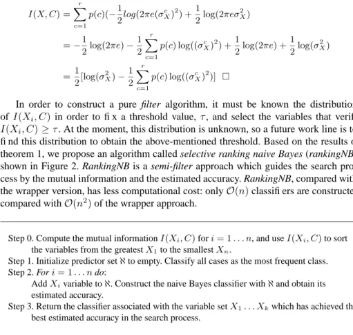
In order to construct a pure filter algorithm, it must be known the distribution of I(Xi, C)in order to fix a threshold value,τ, and select the variables that verify
I(Xi, C)≥τ. At the moment, this distribution is unknown, so a future work line is to
find this distribution to obtain the above-mentioned threshold. Based on the results of theorem 1, we propose an algorithm called selective ranking naive Bayes (rankingNB) shown in Figure 2. RankingNB is a semi-filter approach which guides the search pro-cess by the mutual information and the estimated accuracy. RankingNB, compared with the wrapper version, has less computational cost: onlyO(n)classifiers are constructed compared withO(n2)of the wrapper approach.
Step 0. Compute the mutual informationI(Xi, C)fori= 1. . . n, and useI(Xi, C)to sort
the variables from the greatestX1to the smallestXn.
Step 1. Initialize predictor setℵto empty. Classify all cases as the most frequent class. Step 2. Fori= 1. . . ndo:
AddXivariable toℵ. Construct the naive Bayes classifier withℵand obtain its
estimated accuracy.
Step 3. Return the classifier associated with the variable setX1. . . Xkwhich has achieved the
best estimated accuracy in the search process.
Fig. 2. Proposed selective ranking naive Bayes algorithm.
Due to the independence assumption, the factorization represented by the structure is as simple as the nB factorization shown in Equation 3. For example, the factorization of Figure 1(b) results inp(c|x)∝p(c)f(x1|c)f(x2|c)f(x4|c).
2.3 Semi naive Bayes
The Semi naive Bayes (semiNB) classifier [12, 23] breaks with the strong independence assumption of NB. With this purpose, a new kind of variable called joint variableYkis
presented. This kind of variable is composed by the joint of some of the original vari-ables, where each of the original variables can be in nor more than one joint variable. The fact that two variables,XiandXj, compose a joint variable,Yk, implies that these
two variables are correlated, assuming that they are not conditionally independent. If a joint variable is composed of multinomial random variables, the states of the joint vari-able consist in the cartesian product of the states of the multinomial random varivari-ables [23]. The main problem of joint variables composed by multinomial variablesXi is
the estimation of their class conditional probability tables because they have a number of exponential states inmk,Q mk i=1r (k) i −1, wherer (k)
i is the number of states of the
multinomial random variableXi(k), andmkis the number of original variables which
constitute the joint variableYk.
If a joint variable is composed of a set of Gaussian variables, it follows a multidi-mensional normal distribution [1] conditioned to the class variable. This is one of the contributions of this work. The joint node distribution function follows:
f(yk |c) = (2π)−12mk |Σc k|− 1 2 e−12(yk−µ c k) t (Σc k) −1 (yk−µ c k) (4) where Σc
k is the covariance matrix conditioned to a class value, andµ c
k is the mean
vector conditioned to a class value of the joint variable Yk. In order to model this
distribution function a number of parametersm2
k ∗ris needed. This fact solves the
problem of the probability table size needed to model the joint variable relation with the class variable when the component random variables are considered multinomial.
Depending on the direction of the greedy search process (forward and backward) Pazzani [23] presents two ways to detect dependencies among variables. Our adapta-tion of the called Forward Sequential Selecadapta-tion and Joining (FSSJ) to handle continuous variables is based on Equation 4 to model the class dependence relation of joint vari-ables. The adaptation of the algorithm in a backward search direction can be easily done by the application of the same equation.
The FSSJ algorithm initializes the set of variables to be used by the Bayesian classi-fiers to an empty set. It considers two operators to do the search in the space of possible structures:
1. Add a variable not used by the current classifier as a new variable class condition-ally independent of all other variables used in the classifier.
2. Joint a variable not used by the current classifier with a variable currently used by the classifier.
At each step in the classifier construction, every addition and every joining of an unused variable with a used variable is considered and evaluated by the estimated accuracy using a leave one out validation on the training data. If no change makes an accuracy improvement, the current classifier is returned.
This is a pure wrapper algorithm that constructsO(2n)classifiers. A future work
line consists in the implementation of a filter semiNB version based on (CFS) feature subset selection.
As semiNB considers independent joint variables, the factorization of a semiNB structure is very similar to the NB factorization. It is obtained from equation 3 using equation 4 instead of 2 to factorize terms likep(Xi|C). For example, the factorization
of the structure shown in figure 1(c), assuming thatY1 = (X1),Y2 = (X2, X3)and
Y3= (X4), results inp(c|x)∝p(c)f(x1|c)f(x2, x3|c)f(x4|c).
2.4 Tree augmented naive Bayes
The tree augmented naive Bayes (TAN) [7, 10] also breaks with the strong indepen-dence assumption made by nB classifier, allowing probabilistic dependencies among predictors.
In this subsection, the adaptation to handle continuous value variables of two well-known algorithms to induce TAN structures among the variables is exposed, corre-sponding to filter [7] and wrapper [10] approaches.
As in the original algorithms, in the filter version (fTAN) the permitted graph struc-tures are limited to tree strucstruc-tures between predictor variables and with arcs from the class variable to all predictors as shown in Figure 1(d). In the wrapper version (wTAN), we allow graphs with arcs from class variable only to selected predictors and with arcs between predictors taking into account that the maximum number of parents of a vari-able is one. It has a forest between predictors varivari-ables instead of the tree structure among predictors.
The well-known fTAN induction algorithm finds the tree structures that maximize the likelihood given the data. It can be considered an adaptation of the algorithm pro-posed by Chow and Liu [2], where they reduce the problem of constructing a maximum likelihood tree to construct a maximal weighted spanning tree in a graph. The algo-rithm proposed by Friedman et al. (1997)(wTAN) follows the general outline of Chow and Liu’s procedure, but instead of using the mutual information between two variables, it uses class conditional mutual information between predictors to construct the maxi-mal weighted tree. In order to adapt this algorithm to continuous variables we need to calculate the mutual information between every pair of predictor variables conditioned by the class variable. The following theorem shows how this computation can be done. Theorem 2. LetC be a multinomial random variable. If the joint density function of variablesXiandXjconditioned toC=cfollows a bivariate normal distribution, then
the mutual information between variablesXiandXjconditioned toCverifies:
I(Xi, Xj |C) =−1/2 r X c=1 p(c) log(1−ρ2 c(Xi, Xj))
Proof. The definition of mutual information betweenXiandXj conditioned to C
ver-ifies that: I(Xi, Xj|C) = r X c=1 p(c)I(Xi, Xj|C=c) =− 1 2 r X c=1 p(c) log(1−ρ2c(Xi, Xj))
The fTAN preserves the Chow-Liu algorithm computational cost, requiring a poly-nomial time in the number of variables [2], and so maintaining nB’s computational sim-plicity. This algorithm has two problems: first, the maximization of the structure likeli-hood does not necessarily imply a minimization of the predictive error. Second, a tree between all predictors should be formed, so several irrelevant relations between vari-ables are inevitably added. In order to solve this problem, Keogh and Pazzani present a wrapper version of the algorithm [10], that we call wrapper tree augmented Bayesian network (wTAN).
The wTAN [10] implies a different approach to constructing tree-augmented Bayesian networks. More than a direct attempt to approximate the underlying probability distribu-tion, they solely concentrate on using the same representation to improve classification accuracy. As the space of possible structures is exponential in number of variables, the authors use a hill climbing greedy search algorithm guided by the estimated accuracy.
For each arc added to the networkO(n2), classifier structures are considered and
evaluated, wherenis the number of predicted variables. In each considered structure O(n), arcs may be added. So the complexity for wTAN isO(n3).
The factorization of the implied TAN structure (in its filter and wrapper versions) is more complex than the case of nB and selectiveNB structures. This is due to the class conditional independence property of groups of variables. The factorization is obtained from equations 1 and 2 taking into account the particularity thatP ai = {Xj, C}or
P ai={C}. For example, the factorization of the Figure 1(d) is:
p(c|x)∝p(c)f(x1|x2, c)f(x2|x3, c)f(x3|c)f(x4|x3, c).
2.5 K-dependence Bayesian classifier
Sahami (1996) introduces an algorithm called k-dependence Bayesian classifier [25] kDB. This framework can be regarded as a spectrum of allowable dependence in a given probabilistic model with the NB algorithm at the most restrictive end and the learning of full BN at the most general extreme.
We regard the structure of the kDB as the structure of the NB which allows each predictorXito have a maximum ofkpredictor variables as parents, apart fromC. In
other words, | P ai |≤ k+ 1[25]. As in the case of TAN paradigm, there are two
reasons to restrict the number of parents of a variable. First, the reduction of the search space. Second, the probability estimated for a multinomial variable becomes more un-reliable as additional multinomial parents are added, because the size of the conditional probability tables increases exponentially with the number of parents [10] and fewer cases can be used to compute the needed statistics. As explained in the introduction of Section 2, the number of required parameters in our continuous adaptations is fixed, so the second problem is avoided. In addition to estimating these parameters, instead of learning from database partition, the entire database is used. This allows to construct classifiers with a high number of dependencies between variables.
As the implementation of the kDB algorithm proposed by Sahami [25] uses the class conditional mutual information between the variablesI(Xi, Xj |C)and the mutual
in-formation between class and the variablesI(Xi, C)to lead the structure search process,
it is considered a filter paradigm. Hence, we call his approach fkDB. In the introduced continuous adaptation, the introduced mutual information definitions, shown in equa-tions 1 and 2, are used again. The fkDB algorithm allows the construction of classifiers at arbitrary values for the maximum number of dependencies between variables (values ofk), maintaining much of the computational efficiency of the nB model.
At this point we present the novel wrapper approach of kDB called wkDB. wkDB has the same motivation as wTAN with respect respect to fTAN. The wkDB algorithm follows the idea of Keogh and Pazzani’s [10] wTAN with Friedman et al’s [7] fTAN algorithm introducing the parameterK, for eachi,1< i < n,|P ai| ≤K+ 1, where
K is the number of continuous variables. Our novel wkDB algorithm is shown in Figure 3.
The factorization of kDB and TAN structures are equivalent. For example, the fac-torization of Figure 1(e) is:
Step 1. Initialize predictor set to empty. Classify all the cases as the most frequent class. Step 2. Repeat in each step. Select the best between:
(a) Each variable not included in the model is considered a new predictor. This new predictor must be conditionally independent with respect to the others given, the class. (b) Include an arcαi,jbetween predictors included in the modelXi, Xj, i6=j,
as long as the inclusion ofαi,jcomes with the k-dependent Bayesian classifier
structure.
Evaluate each possible option through the correct classified percentage. Until No option improves the inducted classifier.
Fig. 3. Proposed wkDB algorithm.
3
Experimental results
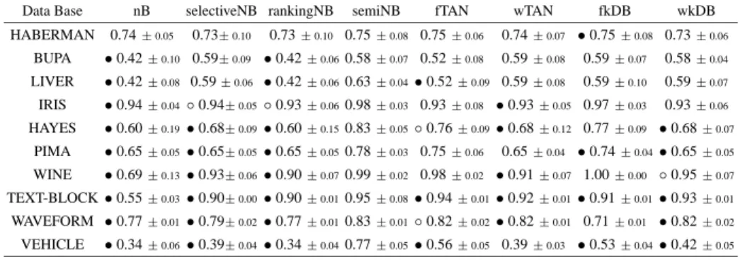
In this section, we present the estimated predictive accuracies and Brier score values [22, 26] obtained with the models of the adapted GN classifier learning algorithms. The results have been obtained in eleven UCI repository data sets [20] which only contain continuous predictor variables. All the included databases, except waveform, do not obey the assumption that variables follow a Gaussian distribution, done by Gaussian network paradigm. In spite of that, the classifiers presented in this work obtains results comparable to their discrete versions.
The results for each classifier in each database have been obtained by a 10-fold cross-validation process with both scores. The performed study has been divided in three steps, with both scores:
1. Select the classifier with the better score average, taking into account the estimated score for each database.
2. Based on the 10-fold cross-validation score estimation, for each classifier in all databases, establish if the selected classifier has obtained better estimated scores at
α= 5%significance level in a paired Wilcoxon [6] test.
3. Based on the scores obtained with each fold of the 10-fold cross-validation process, for each classifier in each database, establish if the selected classifier has obtained better results than others in a non-paired Mann-Whitney[6] test. The study has been performed atα = 10%andα = 5%significance levels, represented in Tables 1 and 2 by “◦” and “•” respectively. The tested databases are presented in tables in order of the number of parameters needed to model a complete Gaussian network (proportional ton∗r).
3.1 Estimated predictive accuracy
The results obtained are summarized in Table 1. The classifier with the best estimated score average is semiNB. A conclusion drawn from the second step of the study is that semiNB has obtained better estimated scores atα= 5%significance level in the selected databases. The third step of the study suggests that the accuracy differences obtained by the semiNBare more statistically significant as the number of needed parameters to model a complete graph increases.
Data Base nB selectiveNB rankingNB semiNB fTAN wTAN fkDB wkDB HABERMAN 0.74±0.05 0.73±0.10 0.73±0.10 0.75±0.08 0.75±0.06 0.74±0.07 •0.75±0.08 0.73±0.06 BUPA •0.42±0.10 0.59±0.09 •0.42±0.060.58±0.07 0.52±0.08 0.59±0.08 0.59±0.07 0.58±0.04 LIVER •0.42±0.08 0.59±0.06 •0.42±0.060.63±0.04•0.52±0.09 0.59±0.08 0.59±0.10 0.59±0.07 IRIS •0.94±0.04◦0.94±0.05◦0.93±0.060.98±0.03 0.93±0.08 •0.93±0.05 0.97±0.03 0.93±0.06 HAYES •0.60±0.19•0.68±0.09•0.60±0.150.83±0.05◦0.76±0.09•0.68±0.12 0.77±0.09 •0.68±0.07 PIMA •0.65±0.05•0.65±0.05•0.65±0.050.78±0.03 0.75±0.06 0.65±0.04 •0.74±0.04•0.65±0.05 WINE •0.69±0.13•0.93±0.06•0.90±0.070.99±0.02 0.98±0.02 •0.91±0.07 1.00±0.00 ◦0.95±0.07 TEXT-BLOCK•0.55±0.03•0.90±0.00•0.90±0.010.95±0.08•0.94±0.01•0.92±0.01•0.91±0.01•0.93±0.01 WAVEFORM •0.77±0.01•0.79±0.02•0.77±0.010.83±0.01◦0.82±0.02•0.82±0.01 0.71±0.01 •0.82±0.02 VEHICLE •0.34±0.06•0.39±0.04•0.34±0.040.77±0.05•0.56±0.05 0.39±0.03 •0.53±0.04•0.42±0.05 Average 0.58 0.70 0,65 0.82 0.74 0.72 0.70 0.74
Table 1. Estimated accuracy results.
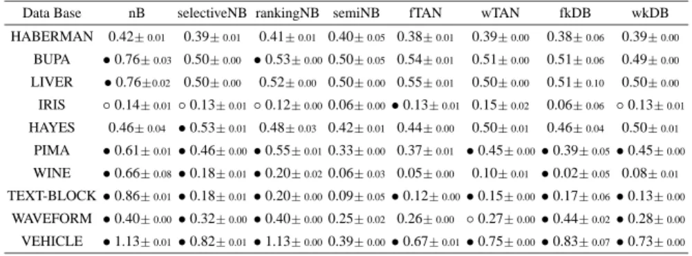
3.2 Estimated Brier score
The Brier score reflects the mean confidence of the learned classifier in the real class of the training data. The formulation of the Brier score is shown in Equation 5:
B = N X l=1 r X c=1 (p(C=c|X=x(l))−δ(l) c )2 (5)
where p(c|x(l))function is factorized by the classifier,x(l)represents the values for predictive variables of the casel,N is the number of cases, andδ(l)c is the Kronecker
delta. The Kronecker delta is defined as follows: δ(cl)=
1c=c(l) 0otherwise
wherec(l)is the real class of the casel, andcis the predicted class value. A high Brier
score indicates that the learned classifier assigns low confidence levels to the real class of the instances.
The problem is thatf function must be a probability andPr
c=1f(C = c | X =
x(l)) = 1. Discrete classifiers directly handle probabilities and so comply with this idea, but continuous classifiers must be normalized because they handle distribution functions (Equations 1 and 2) instead of probabilities. The normalization of the discrete classifierf process is given by
ρ(C=c(l)|X=x(l)) = f(C=c (l)|
X=x(l)) Pr
c=1f(C=c|X=x(l))
The obtained results for the Brier score are summarized in Table 2. The performed study throws similar results than the estimated accuracy study, highlighting the compet-itive results of semiNB.
4
Conclusions and future work
A battery of filter and wrapper classifiers, based on Gaussian networks, is proposed to deal with continuous variables without discretizing them. The classifiers have been compared in 7 databases with two different scores: estimated accuracy and Brier score.
Data Base nB selectiveNB rankingNB semiNB fTAN wTAN fkDB wkDB HABERMAN 0.42±0.01 0.39±0.01 0.41±0.01 0.40±0.05 0.38±0.01 0.39±0.00 0.38±0.06 0.39±0.00 BUPA •0.76±0.03 0.50±0.00 •0.53±0.000.50±0.05 0.54±0.01 0.51±0.00 0.51±0.06 0.49±0.00 LIVER •0.76±0.02 0.50±0.00 0.52±0.00 0.50±0.00 0.55±0.01 0.50±0.00 0.51±0.10 0.50±0.00 IRIS ◦0.14±0.01◦0.13±0.01◦0.12±0.000.06±0.00•0.13±0.01 0.15±0.02 0.06±0.06 ◦0.13±0.01 HAYES 0.46±0.04 •0.53±0.01 0.48±0.03 0.42±0.01 0.44±0.00 0.50±0.01 0.46±0.04 0.50±0.01 PIMA •0.61±0.01•0.46±0.00•0.55±0.010.33±0.00 0.37±0.01 •0.45±0.00•0.39±0.05•0.45±0.00 WINE •0.66±0.08•0.18±0.01•0.20±0.020.06±0.03 0.05±0.00 0.10±0.01 •0.02±0.05 0.08±0.01 TEXT-BLOCK•0.86±0.01•0.18±0.01•0.20±0.000.09±0.05•0.12±0.00•0.15±0.00•0.17±0.06•0.13±0.00 WAVEFORM •0.40±0.00•0.32±0.00•0.40±0.000.25±0.02 0.26±0.00 ◦0.27±0.00•0.44±0.02•0.28±0.00 VEHICLE •1.13±0.01•0.82±0.01•1.13±0.000.39±0.00•0.67±0.01•0.75±0.00•0.83±0.07•0.73±0.00 Average 0.69 0.45 0,50 0.28 0.38 0.40 0.40 0.36
Table 2. Estimated Brier results
In sum, semiNB obtains statistically significant improvements (using accuracy and Brier score) with respect to the rest of the algorithms in the presented databases.
Table 3 presents a work summary: the proposed novel contributions and the adapta-tions of previous works to the continuous domains presented in the article.
nB selectiveNB rankingNB semiNB fTAN wTAN fkDB wkDB adapted adapted novel adapted adapted adapted adapted novel
Theorem 1 Equation 4 Theorem 2
Table 3. Contributions of the article in each included algorithm.
A future work line, related to the wrapper approach, consists in the adaptation of more classifiers supported by BNs for operating directly with continuous variables. The idea consists in the use of randomized heuristics (such as Genetic Algorithms or Es-timation Distribution Algorithms [15]) as the search engine in the space of classifier structures. Following with the wrapper approaches, the Brier score shows the confi-dence of the classifier in the real class more in depth than accuracy. This fact suggests that it could be interesting to use the Brier score, instead of accuracy, to lead the struc-ture search.
Another work line consists in obtaining a threshold for the mutual information intro-duced here (Equations 1 and 2). This will allow us to implement a pure filter algorithm based on the mentioned thresholds. Following with the filter approaches, a possible future work is the implementation of a semi naive Bayes classifier based on the Cor-relation Based Feature Selection [9] to select the groups of variables highly correlated with the class and not correlated among them.
Finally, another interesting study could consist in obtaining the results for Brier score and estimated accuracy using two new validation methods called conservative Z and corrected resampled t-test [21], instead of the used K-Fold cross-validation.
5
Acknowledgments
This work was supported in part by a PhD purpose grant of the Basque Government, by the ETORTEK-GENMODIS and ETORTEK-BIOLAN projects from the Basque Government, and by the University of the Basque Country under 9/UPV 00140.226-15334/2003 grant.
References
1. F. W. Anderson. An Introduction to Multivariate Statistical Analysis. John Wiley and Sons, 1958.
2. C. Chow and C. Liu. Approximating discrete probability distributions with dependence trees. IEEE Transactions on Information Theory, 14:462–467, 1968.
3. T. M. Cover and J. A. Thomas. Elements of Information Theory. John Wiley and Sons, 1991. 4. P. Domingos and M. Pazzani. On the optimality of the simple Bayesian classifier under
zero-one loss. Machine Learning, 29:103–130, 1997.
5. R. Duda and P. Hart. Pattern Classification and Scene Analysis. John Wiley and Sons, 1973. 6. E. J. Dudewicz and S. N. Mishra. Moderm Mathematical Statistics. 1988.
7. N. Friedman, D. Geiger, and M. Goldszmidt. Bayesian network classifiers. Machine Learn-ing, 29:131–163, 1997.
8. D. Geiger and D. Heckerman. Learning Gaussian networks. Technical report, Microsoft Research, Advanced Technology Division, 1994.
9. M. A. Hall and L. A. Smith. Feature subset selection: A correlation based filter approach. In Proceeding of the Fourth International Conference on Neural Information Processing and Intelligent Information Systems, pages 855–858, 1997.
10. E. J. Keogh and M. Pazzani. Learning augmented Bayesian classifiers: a comparison of distribution-based and non distribution-based approaches. In Proceedings of the 7th Inter-national Workshop on Artificial Intelligence and Statistics, pages 225–230, 1999.
11. R. Kohavi and G. John. Wrappers for feature subset selection. Artificial Intelligence, 97(1-2):273–324, 1997.
12. I. Kononenko. Semi-na¨ıve Bayesian classifiers. In Proceedings of the 6th European Working Session on Learning, pages 206–219, 1991.
13. P. Langley, W. Iba, and K. Thompson. An analysis of Bayesian classifiers. In Proceedings of the 10th National Conference on Artificial Intelligence, pages 223–228, 1992.
14. P. Langley and S. Sage. Induction of selective Bayesian classifiers. In Proceedings of the 10th Conference on Uncertainty in Artificial Intelligence, pages 399–406, 1994.
15. P. Larra˜naga and J. A. Lozano. Estimation of Distribution Algorithms. A New Tool for Evo-lutionary Computation. Kluwer Academic Publishers, 2002.
16. S. L. Lauritzen. Graphical Models. 1996.
17. H. Liu and H. Motoda. Feature Selection for Knowledge Discovery and Data Mining. Kluwer Academic Publishers, 1998.
18. DeGroot M. Optimal Statistical Decisions. McGraw-Hill, New York, 1970.
19. M. Minsky. Steps toward artificial intelligence. Transactions on Institute of Radio Engineers, 49:8–30, 1961.
20. P. M. Murphy and D. W. Aha. UCI repository of machine learning databases. Technical report, University of California at Irvine. http://www.ics.uci.edu/∼mlearn, 1995.
21. C. Nadeau and Y. Bengio. Inference for the generalization error. Machine Learning, 52:239– 281, 2003.
22. H.A. Panofsky and G.W. Brier. Some Applications of Statistics to Meteorology. The Penn-sylvania State University, Univesity Park, PennPenn-sylvania, 1968.
23. M. Pazzani. Searching for dependencies in Bayesian classifiers. In Learning from Data: Artificial Intelligence and Statistics V, pages 239–248, 1997.
24. J. Pearl. Probabilistic Reasoning in Intelligent Systems: Networks of Plausible Inference. Morgan Kaufmann Publishers, 1988.
25. M. Sahami. Learning limited dependence Bayesian classifiers. In Proceedings of the 2nd International Conference on Knowledge Discovery and Data Mining, pages 335–338, 1996. 26. L.C. van der Gaag and S. Renooij. Evaluation scores for probabilistic networks. In Proceed-ings of the 13th Belgium-Netherlands Conference on Artificial Intelligence, pages 109–116, Amsterdam, The Netherlands: Universiteit van Amsterdam, 2001.