Study of the relationship between the EEG and BOLD signals using intracranial EEG - fMRI data simultaneously acquired in humans

(1)

Success is not final, failure is not fatal, it is the courage to continue that counts.

(2)

(3)

Study of the relationship between

the EEG and BOLD signals using intracranial EEG - fMRI data

simultaneously acquired in humans

Teresa Inês Gonçalves Murta

Department of Clinical and Experimental Epilepsy Institute of Neurology

University College London

(4)

Personal Statement

I, Teresa Inês Gonçalves Murta, confirm that the work presented in this thesis is my own. Where information has been derived from other sources, I confirm that this has been indicated in the thesis.

Financial Support

This work was conducted through the support of the Foundation for Science and Technology (FCT) grant SFRH/BD/80421/2011 (Bolsa de Doutoramento (BD) individual atribuída a Teresa Inês Gonçalves Murta), and project grants PTDC/BBB-IMG/2137/2012 and LARSyS [UID/EEA/50009/2013], Portugal; Medical research centre, grant G0301067, United Kingdom; and National Institute for Health Research UCL Hospitals Biomedical Research Centre, United Kingdom.

(5)

Table of Figures

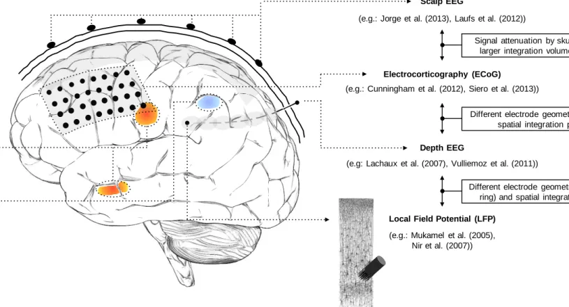
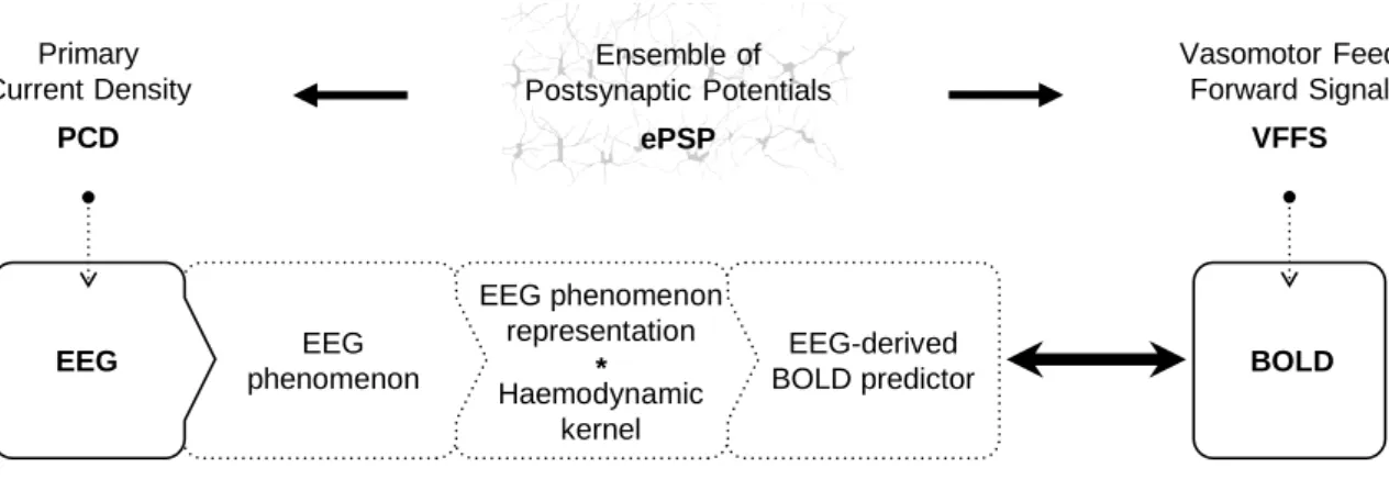
Figure 1-1 Common pipeline of EEG-informed fMRI in epilepsy. Functional MRI is used to map the generators of interictal activity, visually identified in the simultaneously recorded EEG. Matrix design example borrowed from Chaudhary et al. (2012b). EEG traces and fMRI maps illustrations borrowed from Vulliemoz et al. (2011). ... 19 Figure 2-1 Brain signals at multiple scales: from thousands of neurons to whole-brain. Illustration of recording of scalp EEG, ECoG, depth EEG and LFP signals, and three hypothetical BOLD-fMRI clusters, in different lobes. The spatial sensitivity profiles of the four electrophysiological techniques are sketched in shaded grey: mainly neocortical for scalp EEG and ECoG, local to each electrode pair for depth EEG (~1cm3_{), and local to each microelectrode for LFP (~100µm}3_).

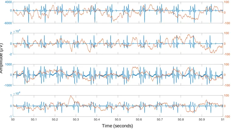
LFP recording is illustrated using a drawing from (Ramón y Cajal, 1899). ... 26 Figure 2-2 General EEG-informed fMRI integration scheme, highlighting the mechanisms underlying each signal. In a given voxel, the neuronal activity generates an ensemble of postsynaptic potentials (ePSP). The temporarily and spatially synchronised summated PSP produce the primary current sources (PCD). The head volume conductor properties transform the PCD into EEG. The ePSP generates a vasomotor feed forward signal (VFFS), via its own forward model, which is in turn transformed, via the haemodynamic forward model, into the observed BOLD signal. ePSP, PCD, VFFS, EEG, and BOLD are time-dependent. The EEG is considered to have the same time evolution as the PCD, which is considered to be a driver for the BOLD signal. This is an asymmetrical EEG and fMRI data integration approach because the EEG temporal dynamics are taken as surrogates for the VFFS. Diagram adapted from Valdes-Sosa et al. (2009). ... 32 Figure 3-1 Examples of icEEG signal power spectra after the gradient artefact correction. Different colours represent different icEEG contacts (located over the motor cortex). ... 54 Figure 3-2 Example of CT and T1 images. Blue arrow highlight icEEG contacts. Red arrow highlights a group of high intensity voxels that it is not a icEEG contact. ... 55 Figure 3-3 Illustration of the clustering algorithm designed by me to find the coordinates of the icEEG contacts. In this example, the final solution (i.e. coordinates of the contacts) is found after two iterations. ... 56 Figure 4-1 Representative icEEG time courses (Patient IH; see an illustration of the icEEG implantation scheme in Figure 4-3), before (blue) and after (orange) the subtraction of the gradient artefact template. Note the different scales of the y-axes. In this example, the artefact template was computed with the sequential average approach, using 51 data epochs (k=51). ... 64 Figure 4-2 Internal scanner ventilation artefact time-frequency characterisation in the eigenvariates space. Time-frequency amplitude profile (Morlet wavelet factor: 1800; y-axis samples: 100) of the first three eigenvariates, for the frequency range 92.7 - 93.7 Hz, obtained by a SVD of the band-pass filtered icEEG signal. ... 69

(11)

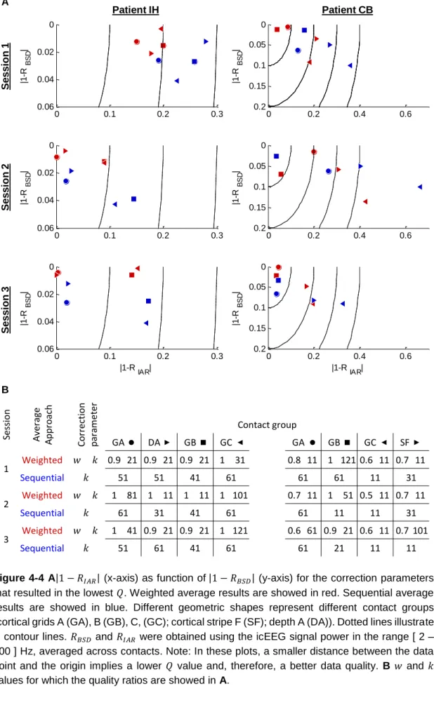
Figure 4-3 IcEEG implantation scheme for patients IH, on the left, and CB, on the right. ... 70 Figure 4-4 A1-RIAR (x-axis) as function of 1-RBSD (y-axis) for the correction parameters that resulted in the lowest Q. Weighted average results are showed in red. Sequential average results are showed in blue. Different geometric shapes represent different contact groups (cortical grids A (GA), B (GB), C, (GC); cortical stripe F (SF); depth A (DA)). Dotted lines illustrate Q contour lines. RBSD and RIAR were obtained using the icEEG signal power in the range [ 2 – 200 ] Hz, averaged across contacts. Note: In these plots, a smaller distance between the data point and the origin implies a lower Q value and, therefore, a better data quality. B w and k values for which the quality ratios are showed in A. ... 71 Figure 4-5 Translations, arc of rotation (x displayed in blue, y in green, z in red, and x2 + y2 + z2 in black) and motion events *, which represent fMRI volumes where the total differential motion was above 0.2 millimetres. ... 72 Figure 4-6 Internal scanner ventilation artefact time-frequency characterisation, in the contacts space. Power spectra for the frequency range [ 90 - 96 ] Hz are shown on the top right, and time-frequency amplitude profiles for the time-frequency range [ 92.7 - 93.7 ] Hz are shown on the bottom, of two representative icEEG contacts. ... 74 Figure 4-7 Cooling compression pump artefact correction effect. Spectra for the frequency range [ 90 - 120 ] Hz of three representative icEEG contacts. Data corrected for gradient and cooling pump related artefacts are presented in red, overlying data only corrected for gradient artefacts, presented in black. Blue boxes highlight the cooling pump artefact peaks. Green boxes highlight the ventilation artefact peaks. Yellow boxes highlight residual gradient artefact peaks. ... 75 Figure 4-8 Internal scanner ventilation artefact correction effect. Power spectra for the frequency range [ 90 - 96 ] Hz (top right), and time-frequency amplitude profiles for the frequency range [ 92.7 - 93.7 ] Hz (bottom), of two representative icEEG contacts, after gradient and internal ventilation artefact corrections. ... 76 Figure 5-1 Design matrices of all the BOLD signal models considered. The regressor of interest, i.e. the regressor that was orthogonalised with respect to the combination of the others, is highlighted in dark grey. ... 91 Figure 5-2 Finger tapping related BOLD increases (t-contrast, p<0.001, uncorrected). ... 92 Figure 5-3 Patient-specific  and  bands of interest. Fractal and harmonic spectra for the ipsilateral finger tapping periods, computed using a coarse-graining spectral analysis (CGSA) (Yamamoto and Hughson, 1991), as described in He et al. (2010). ... 94 Figure 5-4 Contact pairs of interest. A ECoG contacts (black), and finger tapping BOLD increases (red). B Spectral differences for contralateral and ipsilateral finger tapping periods. C Pre-surgical electrical stimulation results. Contacts showing peaks of apparent artefactual origins (harmonic high-amplitude peaks (prominent residual gradient artefacts), or a 50 Hz

(12)

(electrical component) high-amplitude peak) were not analysed, and are displayed as a dotted cross. ... 95 Figure 5-5 EEG band power – BOLD amplitude correlation. Pearson’s linear correlation coefficients between the power of multiple EEG frequency components and the amplitude of the contralateral finger tapping - related BOLD time course. The grey tone identifies the distance between the ECoG contact pair (middle distance between the two contacts) and the maximum t-value of the cluster of significant contralateral finger tapping - related BOLD changes. ... 96 Figure 5-6 Influence of the EEG  and  phases in the EEG  power - BOLD amplitude correlation. Pearson’s linear correlation coefficients between the power of multiple EEG frequency components and the amplitude of the finger tapping - related BOLD time course, when the  power was segmented according to the  phase (on the left) or the  phase (on the right). The curve colour identifies the phase bin according to which the  power was segmented. .... 97 Figure 5-7 { , γ } and { , γ } frequency pairs of interest. Phase-amplitude comodulogram plots (z-scored PAC strength values) for the patient-specific  and  bands, obtained with the Canolty metric (p < 0.05; corrected for multiple comparisons using Bonferroni criterion). ... 98 Figure 5-8 BOLD signal changes GLM results. t-values for the PACβγ, Pα, Pβ, and Pγ effects.

Different shapes represent different patients. Filled shapes represent t-values with p < 0.05. 99 Figure 5-9 Cross-correlation matrices.PairwisePearson's linear correlation coefficients for all EEG-derived regressors and BOLD time course of interest. No values are shown for PACαγ for

patient LT and CB because no significant PAC effect was found for the α band of these patients. ... 99 Figure 6-1 Representative EEG time courses (patient HD) showing sharp waves of different amplitudes and widths (blue arrows point at events visually marked at COI: DA 3 – 4). ... 110 Figure 6-2 Average IED for each set of events of interest (SCOI). ... 111 Figure 6-3A - D Sharp wave morphology-based features: A amplitude, B width, C rising phase slope, D energy, overlaid on an example of a single-trial IED estimate. E - F Single-trial IED estimates examples. The original IED is displayed in black, the average IED is displayed in grey, and the estimated IED is displayed in blue. ... 116 Figure 6-4 Representative example (patient BS, events of interest set: S2, see... 119 Figure 6-5 Variance explained (VE) results. Experiments level analysis: A Average VE values, by modulatory feature; for the set of voxels comprised in pBOLD, and D in nBOLD. Group level analysis: B Average VE and respective standard deviation values, by modulatory feature; for the set of voxels comprised in pBOLD, and D in nBOLD. Undefined values correspond to cases where no voxel had a large enough t-value to survive the threshold used (p < 0.05, uncorrected). ... 120 Figure A-1 Phase-amplitude comodulogram plots obtained using three different PAC strength estimation metrics, for each patient-specific COI. The plots obtained with Canolty’s and Tort’s

(13)

metrics are thresholded at p < 0.05 and corrected for multiple comparisons using the Bonferroni criterion... 160 Figure A-2 BOLD signal changes GLM results. t-values for the PACβγ, Pα, Pβ, and Pγ effects.

Different colours represent different PAC strength metrics. Different shapes represent different patients. Filled shapes represent t-values with p < 0.05. ... 161 Figure A-3 BOLD signal changes GLM results. t-values for the PACβγ, Pα, Pβ, and Pγ effects. Different colours represent different epoch durations for the estimation of the PAC strength. Different shapes represent different patients. Filled shapes represent t-values with p < 0.05. ... 161

(14)

Table of Tables

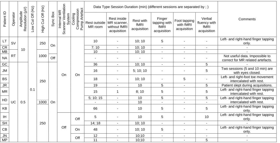
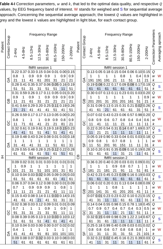
Table 3-I Description of the icEEG-fMRI data acquisitions: icEEG recording parameters, scanner-related factors, and experimental protocols. ... 53 Table 4-I Correction parameters, w and k, that led to the optimal data quality, and respective Q

values, by EEG frequency band of interest. W stands for weighed and S for sequential average approach. Concerning the sequential average approach; the lowest Q values are highlighted in grey and the lowest k values are highlighted in light blue, for each contact group. ... 73 Table 5-I IcEEG implantation characterisation: types of electrodes, number of contacts per electrode, and implantation scheme. The ECoG contact pairs analysed (over the motor cortex) are highlighted with numbered black squares. FLE: Frontal lobe epilepsy, R: right, L: left, A: anterior, M: medial, P: posterior, I: inferior, and S: superior. ... 93 Table 6-I Description of SCOI and sharp wave feature estimates for BOLD modelling. FW: focal

plus more widespread, F: focal. ... 111 Table 6-II IcEEG implantation characterisation: type of electrodes, number of contacts per electrode, and implantation scheme. TLE: Frontal lobe epilepsy, FLE: Frontal lobe epilepsy, R: right, L: left, A: anterior, M: medial, P: posterior, I: inferior, and S: superior. Intra-contact distances: 10 millimetres for grids, strips, and most depths; 5mm for high-density grids and medial contact pairs in some depths. The approximated location of each COI is highlighted with a green arrow (depth), or square (ECoG). ... 112

(15)

Acronyms

BOLD Blood-oxygen-level-dependent CBF Cerebral blood flow

CBV Cerebral blood volume

CMRO2 Cerebral metabolic rate of oxygen

COI Contact pair of interest DAN Dorsal Attention Network DMN Default Mode Network ECoG Electrocorticography

EEG Electroencephalography, Electroencephalogram EPSP Excitatory post-synaptic potential

ERD Event-related desynchronisation ERP Event-related potential

ERS Event-related synchronisation

fMRI Functional magnetic resonance imaging FWHM Full-width at half-maximum

GLM General linear model HF High-frequency

HRF Haemodynamic response function IC Independent component

ICA Independent component analysis icEEG Intracranial electroencephalography

IED Interictal epileptiform discharge IPSP Inhibitory post-synaptic potential

LF Low-frequency LFP Local filed potential MUA Multi-unit activity

PAC Phase-amplitude coupling PAC Phase-amplitude coupling

PC Principal component

PCA Principal component analysis PCD Primary current sources PSP Post-synaptic potential RSN Resting State Network SEEG Stereotactic EEG

SOZ Seizure onset zone

SPM Statistical Parametric Mapping SUA Single-unit activity

(16)

(17)

The principal aim of this work was to further characterise the relationship between the electrophysiological and BOLD fMRI signals at the local level, exploiting the unique opportunity to analyse intracranial EEG (icEEG) and fMRI data recorded simultaneously in humans, during a finger tapping task and at rest. The MR-environment (gradient switch and mechanical vibration) related artefacts corrupting the icEEG data were the first problem tackled; they were characterised and removed using techniques developed by me. The two parts that followed aimed to shed further light on the neurophysiological basis of the BOLD effect. Firstly, the influence of the phase of the low frequency EEG activities (< 30 Hz) on capability of an EEG power - based model to predict the amplitude of finger tapping related BOLD changes was investigated; the strength of the coupling between the phase of  and the amplitude of  (>70 Hz) (phase-amplitude coupling: PAC) was found to explain variance in addition to a combination of , , and  band powers, suggesting that PAC strength and power fluctuations result from complementary neuronal processes. Secondly, five interictal epileptiform discharge (IED) morphology and field extent related features were tested in their individual capability to predict the amplitude of the co-localised BOLD signal; these were the amplitude and rising phase slope, thought to reflect the degree of neuronal activity synchrony; width and energy, thought to reflect the duration of the excitatory post-synaptic potentials; and spatial field extent, thought to reflect the spatial extent of the surrounding, synchronised sources of neuronal activity. Among these features, the IED width was the only one found to explain BOLD signal variance in addition to the IED onsets, suggesting that the amplitude of the BOLD signal is comparatively better predicted by the duration of the underlying field potential, than by the degree of neuronal activity synchrony.

(18)

(19)

1

(20)

In the last century, human brain activity has been recorded most commonly as electrical potentials on the scalp (scalp electroencephalography - EEG), neocortex surface (electrocorticography - ECoG), or deep inside the brain (depth EEG). Since the early 1990s, using blood-oxygen-level-dependent (BOLD) functional magnetic resonance imaging (fMRI) to record changes in the local blood oxygenation has become an increasingly important tool, largely due to its non-invasive whole-brain coverage and relatively high spatial resolution. These indirect measurements of neuronal activity have been used to study a wide range of processes and phenomena, ranging from sensory or cognitive functions, to sleep or rest stages (which sometimes include spontaneous epileptic discharges). Combining electrophysiological and BOLD fMRI signals emerged as a natural consequence of the complementarity of their temporal and spatial resolutions, and the potential capability of fMRI to locate scalp EEG generators, while bypassing the scalp EEG inverse problem. Simultaneously recorded scalp EEG and BOLD fMRI data have been used to locate brain regions involved in the generation and propagation of epileptic seizures (Chaudhary et al., 2012a; Murta et al., 2012) and interictal epileptiform discharges (IED) (Caballero-Gaudes et al., 2013). The accurate delineation of these regions is the main purpose of the pre-surgical evaluation performed in patients with drug-resistant epilepsies because the best treatment available is to surgically disrupt them. Most studies combining EEG and fMRI data are asymmetric data integration strategies that use the EEG to capture characteristic temporal patterns (e.g.: epileptic spikes, seizure activity, sleep stages, ongoing brain rhythms, etc.) and the fMRI to locate the generator(s) of such activity (Figure 1-1). These strategies are often called EEG-informed fMRI.

Despite extensive investigations and discussions over recent years, we are still not completely aware of the aspects of neuronal processing which are most closely related to the BOLD signal, or about their generality across brain regions and between normal and pathological activities (Ekstrom, 2010; Logothetis, 2010, 2008; Magri et al., 2012). For instance, both BOLD increases and decreases have been linked to the occurrence of epileptic discharges (Pittau et al., 2013), but BOLD decreases have been thought to reflect neuronal activity decreases (Shmuel et al., 2006), which seem incompatible with the occurrence of epileptic discharges. The neural basis of EEG and BOLD signals are briefly described in the first section of Chapter 2, § 2.1, which help us to understand what is currently known about the electrophysiological correlates of the BOLD signal, extensively described in the second section of Chapter 2, § 2.2.

This project was designed to further characterise the local electrophysiological correlates of the BOLD signal, taking advantage of the unique opportunity to analyse intracranial EEG (icEEG) and BOLD fMRI data recorded simultaneously in humans. As a consequence of better understanding the BOLD signal neuronal correlates, the sensitivity of future EEG-informed fMRI data integration strategies may be improved, and, perhaps, more importantly, their interpretation facilitated. Even the most complex theoretically-based EEG-fMRI data integration approaches rely on assumptions about the local electrophysiological correlates of the BOLD signal, usually

(21)

Figure 1-1 Common pipeline of EEG-informed fMRI in epilepsy. Functional MRI is used to map the generators of interictal activity, visually identified in the simultaneously recorded EEG. Matrix design example borrowed from Chaudhary et al. (2012b). EEG traces and fMRI maps illustrations borrowed from Vulliemoz et al. (2011).

embedded in mathematical models that describe the relationships between the two signals and the underlying neuronal activity. For example, Babajani et al. (2005) and Valdes-Sosa et al. (2009) proposed theoretically-based EEG-fMRI data integration models that relied on Logothetis et al. (2001)’s findings suggesting that local field potentials (LFP) were better predictors of BOLD

IED-related BOLD cluster

EEG-fMRI data integration

General Linear Model (GLM) analysis & Statistical Testing: Location of voxel cluster(s) where BOLD changes are significantly correlated with the temporal occurrence of the events of interest

(e.g.: IED-related BOLD clusters) Design matrix definition

Events of no interest identified on the video recording

(e.g.: eye blinks; eye movements; head jerk; hand movement; speaking; coughing) Epileptic activity of interest

(e.g.: left temporal IEDs - sharp waves)

Epileptic activity of no interest (e.g.: right temporal IEDs - sharp waves; slow waves)

Cardiac artefacts

EEG-derived regressors:

Video-derived regressors: fMRI-derived regressors: fMRI realignment parameters (i.e. motion parameters) Definition of EEG-derived BOLD predictor(s) Visual identification of events of interest in EEG recordings

(e.g.: IEDs) EEG data pre-processing

(imaging acquisition and cardiac pulse related artefacts removal; filtering) IED * Haemodynamic kernel (e.g.: canonical HRF) 30s

(IED peaking timings)

Simultaneous EEG-fMRI data acquisition

fMRI data pre-processing (images realignment; data

spatial smoothing, etc.)

Definition of confounds (i.e.: regressors of no interest) (e.g.: fMRI data realignment

parameters; motion events identified by video)

(22)

fluctuations than single- or multi-unit activities (SUA or MUA) (LFP and (S)MUA measured with microelectrodes implanted in the visual cortex of macaques). Knowing which particular EEG-derived feature(s) (e.g.: ongoing activity power, phase-synchrony, phase-amplitude coupling strength; event-by-event morphological and field extent characteristics) correlate better with the simultaneous and co-localised BOLD signal will probably lead to key insights into the neuronal substrate of the BOLD signal, and therefore help us to interpret the commonly observed BOLD fMRI maps.

Activities of multiple frequency ranges, characteristically associated with sensory, motor, and cognitive events, are commonly observed on electrophysiological recordings (Engel et al., 2001; Jacobs and Kahana, 2010; Varela et al., 2001). Interestingly, these activities appear to hierarchically interact with each other, as the “basic units” of a complex system that seems to regulate how information is processed in the brain, across multiple spatial and temporal scales (Buzsaki et al., 2012; Canolty and Knight, 2010; Hyafil et al., 2015; Lakatos et al., 2005; Palva et al., 2005; Roopun et al., 2008). The interaction between the phase of the low (<30 Hz; LF) and the amplitude of high frequency activities (>30 Hz; HF), often simply called phase-amplitude coupling (PAC), has attracted great interest due to its potential functional role (Axmacher et al., 2010; Buzsáki et al., 2012; Cohen et al., 2009a, 2009b; Kramer et al., 2008; Lakatos et al., 2008; Tort et al., 2009). In brief, the strength of PAC fluctuates in a task-dependent manner, both within and across regions; it goes from no influence to strong influence, and back within a few tenths of a second; it can assume different patterns and be modulated in time differently, within different brain structures (Tort et al., 2008); it is proportional to the intensity of training and level of performance (Dürschmid et al., 2014; Tort et al., 2009). A short literature review on the functional relevance of the LF activities phase and, in particular, on the PAC strength, is presented in the third section of Chapter 2, § 2.3. It is currently known that BOLD changes are better predicted by a combination of power of multiple LF and HF activities rather than by the power of the HF activity alone. However, the electrophysiology-based BOLD signal models previously explored did not account for the temporal dynamics of the phase of the LF activities, nor for its coupling to the amplitude of the HF activity. Taking advantage of the unique opportunity to analyse icEEG and BOLD fMRI data simultaneously recorded in humans performing a finger tapping task, we investigated whether fluctuations in the PAC strength explained variance of the BOLD signal amplitude in addition to fluctuations in the power of the EEG signal at multiple LF and HF bands, at the local level, as described in Chapter 5.

While the aforementioned study aimed to investigate the influence of an important EEG-derived feature (the phase of the LF activities) in the currently accepted best electrophysiology-based model of the BOLD signal, the following study aimed to shed further light on the neuronal basis of the BOLD signal, using the knowledge we already have on the relationship between a group of EEG-derived features and the underlying neuronal activity. For this, five IED morphology and spatial field extent related features - amplitude, rising phase slope, width, energy (area under the curve), and spatial field extent (number of icEEG contacts over which the IED was simultaneously observed) – were estimated, event-by-event, and compared, in terms of

(23)

capability to explain variance of the amplitude of the simultaneous and co-localised BOLD signal, which was not explained by the IED onsets alone, in the surroundings of the most active icEEG contact (likely to be in the immediate vicinity of the neuronal generator), as described in Chapter 6. A literature review of studies with similar aims is presented in the fourth section of Chapter 2, § 2.4.

The two aforementioned studies were designed to exploit the unique opportunity to analyse icEEG and BOLD fMRI data simultaneously acquired in humans (acquisition and pre-processing details described in Chapter 3), recently available after solving a number of challenging technical aspects (Boucousis et al., 2012; Carmichael et al., 2012, 2010). The simultaneity of the acquisition of the two signals is essential to investigate ongoing phenomena and events variability; however, it poses some difficulties, as discussed in the fifth section of Chapter 2, § 2.5. Due to this simultaneity, a number of artefacts corrupt both EEG and MRI data. Of particular relevance to us is the quality of the icEEG data because the accuracy of the estimation of the EEG-derived features of interest (phase and amplitude of multiple frequency EEG components; IED event-by-event morphological and spatial field extent characteristics) may be compromised. Therefore, this project started with an exploratory investigation towards improving the icEEG data quality, as described in Chapter 4.

The general conclusions of this work and potential methodological improvements are discussed in Chapter 7.

(24)

(25)

1_{The first three sections of this chapter were adapted from Murta, T., Leite, M., Carmichael,}

D.W., Figueiredo, P., Lemieux, L., 2015. Electrophysiological correlates of the BOLD signal for EEG-informed fMRI. Hum. Brain Mapp. 36, 391–414.

2

(26)

This chapter starts with a brief description of the neurophysiological origins of the EEG and BOLD signals, in § 2.1, to clarify their complementarity. The second section of this chapter, § 2.2, comprises a review of studies that aimed to improve the neurophysiological interpretation of the commonly observed BOLD fMRI maps, by investigating how the electrophysiological and the BOLD signals relate to each other, in multiple scenarios: epilepsy; non-epileptic spontaneous activity; and cognitive, sensory and motor functions. The reviewed studies were grouped as those using fMRI to map haemodynamic changes associated with a particular electrophysiological phenomenon, discussed in § 2.2.1; and those focused on characterising the local relationship between the electrophysiological and haemodynamic signals, often through systematic comparisons of electrophysiology-derived metrics in terms of their capability to predict BOLD signal fluctuations, discussed in § 2.2.2. The third section of this chapter, § 2.3, comprises a review of the studies supporting the functional relevance of the phase of the low frequency EEG activities and, in particular, of the interaction between the phase of the low and the amplitude of the high frequency EEG activities (PAC), the ongoing EEG phenomenon that was later compared with the also ongoing EEG power for multiple frequency bands, in terms of capability to predict the amplitude of the BOLD signal. The forth section of this chapter, § 2.4, comprises a review of the studies that have investigated the relationship between the morphology of IED (amplitude and duration), events commonly observed on EEG, and the amplitude of the BOLD signal. Finally, in the fifth section of this chapter, § 2.5, we discuss the importance of the simultaneity of the EEG and fMRI data acquisition, essential to investigate ongoing phenomena and events variability, and therefore essential to this project, together with the difficulties associated with it. This chapter is focused on human studies, the most relevant for this project, apart from the subsection on the relationship between neuronal spiking rates and the BOLD signal (§ 2.2.2), and a few studies in animals discussed in § 2.4.

2.1 Neural basis of EEG and BOLD signals

In this section, we describe the key aspects of the current understanding of the neurophysiological origin of EEG and BOLD fMRI signals. Cerebral electrophysiological signals (LFP, icEEG, scalp EEG) can be recorded at multiple spatial scales (Figure 2-1). Despite reflecting the underlying neuronal activity differently, these signals related to each other, to a reasonable extent, as discussed in § 2.1.1.1. Most EEG-informed fMRI studies rely on one of the set of electrophysiological phenomena: ongoing (during cognitive, sensory, motor functions, or at rest), event-related, or epileptic activity. These electrophysiological phenomena are briefly described in § 2.1.1.2. The origin of the BOLD effect, together with how its underlying mechanisms may be affected by disease, is discussed in § 2.1.2.

2.1.1 Cerebral electrophysiological signals

Brain function relies on a causal chain of events originated at the level of synapses, the basic elements for communication between neurons. Active neurons generate time-varying electric currents, which result from ions crossing their cellular membranes. There are two main forms of neuronal activation: the slow changes in membrane potential due to synaptic activation, which

(27)

are mediated by several neurotransmitter systems - these are the post-synaptic potentials (PSP; excitatory and inhibitory: EPSP and IPSP); and the fast neuronal membrane depolarisations, which result from action potentials (Lopes da Silva, 2010). The electrical currents arising during synaptic activation can sum to generate electrical potentials that can be measured at different spatial scales (Figure 2-1) (Kajikawa and Schroeder, 2011; Riera et al., 2005).

Most multimodal studies mapping BOLD changes related to particular electrophysiological phenomena use scalp EEG, whereas those focused on characterising the local relationship between the two signals often use LFP, ECoG, or depth EEG (invasive) recordings.

2.1.1.1 Different spatial scales and their relationship to neuronal activity

LFP are recorded with low-impedance microelectrodes placed in the extracellular medium, sufficiently far from individual cells to prevent any particular neuron from dominating the signal, and reflect the activity of several tens of thousands of nerve cells (Fermaglich, 1982). Action potentials (SUA or MUA, depending on the number of cells involved) are obtained by high-pass filtering the extracellular recordings, or by placing the microelectrodes within (or close to) the cell membrane. LFP, SUA, and MUA are rarely recorded in humans due to the required invasiveness.

Due to the particular geometry and hierarchical organisation of neuronal ensembles in some brain structures (e.g.: cortical pyramidal cells arranged parallel to each other, with apical dendrites on one side and soma on the other), PSP can sum into an effective current source. Due to the head tissue conductor properties, this current source can be large enough to be remotely recorded (Niedermeyer and Lopes da Silva, 1999). Scalp EEG primarily reflects the slow EPSP and IPSP of cortical populations (Creutzfeldt et al., 1966a, 1966b; Klee et al., 1965), with some contribution from mechanisms not directly coupled to synaptic activity (e.g.: voltage-dependent membrane oscillations and spike after-potentials) (Buzsaki and Chrobak, 1995; Creutzfeldt et al., 1966a, 1966b; Kandel and Buzsaki, 1997; Kocsis et al., 1999). IcEEG can be recorded in humans with severe drug-resist epilepsy undergoing a clinical pre-surgical evaluation for the curative resective surgery, using macroelectrode arrays (grids or strips) placed over the cortical surface (ECoG), or within the brain (depth EEG; or stereotactic EEG: SEEG). Despite being described as LFP measurements occasionally (Baumgartner et al., 2011; Conner et al., 2011), icEEG2_{measurements represent significantly larger integration volumes than those}

recorded with microelectrodes (Fermaglich, 1982). As consequence of the uncertainty in the location of the epileptic activity generators, icEEG electrodes are often placed over regions that turn out to be apparently free of pathology, which provides an opportunity to study normal brain activity (Conner et al., 2011; Hermes et al., 2012; Khursheed et al., 2011). Clinical icEEG electrodes combined with microelectrodes are not yet in common use, but are a promising research tool (Fried et al., 1999; Hochberg et al., 2006; Schevon et al., 2012; Waziri et al., 2009). .

(28)

Figure 2-1 Brain signals at multiple scales: from thousands of neurons to whole-brain. Illustration of recording of scalp EEG, ECoG, depth EEG and LFP signals, and three hypothetical BOLD-fMRI clusters, in different lobes. The spatial sensitivity profiles of the four electrophysiological techniques are sketched in shaded grey: mainly neocortical for scalp EEG and ECoG, local to each electrode pair for depth EEG (~1cm3_{), and local to each microelectrode for LFP}

(~100µm3_{). LFP recording is illustrated using a drawing from (Ramón y Cajal, 1899).}

26 Uni v ers ity C ol leg e L o nd on T eres a M urt a Positive BOLD changes cluster

Local Field Potential (LFP)

(e.g.: Mukamel et al. (2005), Nir et al. (2007))

Electrocorticography (ECoG)

(e.g.: Cunningham et al. (2012), Siero et al. (2013))

Depth EEG

(e.g: Lachaux et al. (2007), Vulliemoz et al. (2011))

Scalp EEG

(e.g.: Jorge et al. (2013), Laufs et al. (2012))

Negative BOLD changes cluster

Functional MRI (fMRI)

Signal attenuation by skull/scalp and larger integration volume (usually)

Different electrode geometry (disk) and spatial integration profile

Different electrode geometry (cylindrical ring) and spatial integration profile

(29)

The geometry and size of electrodes determines the sensitivity profile of each type of recording. In general, icEEG has greater regional sensitivity and specificity than scalp EEG (approximately 1cm3_{for depth EEG) (Church et al., 1985). In case of deep generators, scalp EEG and ECoG}

are more affected by volume-related averaging effects than depth EEG. Both ECoG and depth EEG have limited spatial sampling because there is a limited number of electrodes that can be used, due to the risks associated with the implantation procedure (Engel, 2013). Despite the high regional specificity, LFP, depth EEG, and ECoG recordings consist of “mean field signals” that result from the collective behaviour of aggregates of neurons; therefore, there is always some ambiguity on the nature of their origin (Buzsaki et al., 2012).

At a larger scale, a particular distribution of electrical potentials recorded on the scalp can be explained by the activity of infinite different configurations of intracranial current sources (Fender, 1987). These current sources are not simple point-like charge accumulations; they have dipolar configurations (Bishop, 1949; Brazier, 1949), which are not simple dipoles, but dipole layers that are convoluted (Bishop, 1949; Gloor, 1985; Vaughn, 1974, 1969). The particular geometry and orientation of these current sources with regard to the electrode contacts are crucial determinants of the potential distribution within the brain or at the scalp (Gloor, 1985; Vaughn, 1974, 1969). Reconstructing the current sources originating the scalp EEG measurements, i.e., solving the scalp EEG inverse problem, is a well-known ill-posed problem with no unique solution. Solving it requires prior assumptions on the number, geometry, and/or location of the current sources, thereby introducing a fundamental uncertainty on the origin of the measured signals (Ferree et al., 2001). Different inverse models are based on different a priori assumptions (for a review see Michel et al. (2004)), and can be categorised as: overdetermined (dipolar) models (e.g.: (Gulrajani et al., 1984; Homma et al., 1990; Kavanagh et al., 1978; Scherg and Von Cramon, 1986; Stok, 1987)), based on the assumption that a small and known number of current sources can adequately model the measurements at the surface; or underdetermined (distributed) source models (e.g.: Pascual-Marqui et al. (1994); Grave de Peralta Menendez et al. (2001)), which reconstruct the brain electric activity in each point of a 3D grid of solution points and do not need an a priori assumption on the number of current sources.

2.1.1.2 Commonly observed electrophysiological activity

FMRI has been used to locate brain regions generating different electrophysiological phenomena, which are briefly explained in the following subsections.

 Epileptiform activity

The electrophysiological signal of patients with epilepsy often encompasses characteristic activity during seizures, also called ictal events, and between seizures, the so-called interictal epileptiform discharges (IED).

In focal epilepsies, the electrophysiological signal at the seizure onset often consists of fast and low-amplitude activity that may spread and become slower and higher in amplitude, and which reflects excessive and hyper-synchronous neuronal activity (Blume et al., 2001). Nevertheless,

(30)

the power-frequency profile of scalp EEG recordings during seizures is highly variable across patients.

IED are high-amplitude fast EEG transients that can last less than 70 milliseconds, and be called interictal spikes, or between 70 and 120 milliseconds, and be called sharp waves. Both spikes and sharp waves are often followed by a slow wave that can last several hundred of milliseconds (De Curtis and Avanzini, 2001). Interictal spikes tend to occur periodically (Chatrian et al., 1964) and often in brief paroxysms, which either remain localised in space or establish a secondary propagation to other parts of the cortex. Interictal spikes reflect the synchronous and excessive discharge of a cortical neuronal ensemble and are associated with a burst discharge, which is characterised by a rapid sequence of fast action potentials at 200 - 500 Hz, superimposed on a slow depolarising potential (De Curtis and Avanzini, 2001).

 Rhythmic and arrhythmic activity

The power spectrum of LFP, icEEG, and scalp EEG signals follows a power law distribution, i.e., it can be broadly represented by a straight line on a logarithmic scale (P(log(f)) ∝ f−c_{, usually} with 0 < c < 4), which characterises the brain arrhythmic activity. Under specific conditions, peaks superimposed to this straight line are observed at particular frequencies. These peaks characterise the brain rhythmic or oscillatory activity (Bullock et al., 2003; Buzsaki and Draguhn, 2004; He et al., 2010).

The brain rhythmic activity, commonly categorised as  (0.5 – 4 Hz),  (4 – 8 Hz),  (8 – 12 Hz), β (12 – 30 Hz), and γ (> 30 Hz) (Lopes da Silva, 2011), seems to be an important element linking neuronal activity and behaviour (Engel et al., 2001; Hasselmo et al., 2002; Somers and Kopell, 1993; Steriade, 2001; Traub et al., 1999; Whittington and Traub, 2003). Despite differences in brain’s sizes of several orders of magnitude, its temporal characteristics are phylogenetically preserved in the mammalian brain. Such preservation throughout evolution has been suggested as evidence that brain rhythmic activity has a specific functional role (see Buzsaki et al. (2013) for further details).

The terms rhythm and oscillation are sometimes applied incorrectly to electrophysiological signals. An increase of the electrophysiological activity within a particular frequency band does not imply the presence of a true rhythm (oscillation) (Lopes da Silva, 2013). Rather, a relatively narrow peak, within the frequency band of interest, must be identifiable in the power spectrum. The rhythm is defined by the central frequency, bandwidth, and power of this peak. To investigate whether a certain peak denotes a rhythm, we can use a period specific average approach, as proposed by Bullock et al. (2003), for example. According to these authors, a rhythm is defined by a narrow peak with frequency modulation of <5 % of the centre frequency, a strength of 2.5 to 10 times the expectation from chance of the background noise, and showing a ﬁne structure by being local and brief (on the order of 10 cycles).

Brain rhythmic activity arises from competition (via inhibition) and cooperation (via excitation) within local micro-networks (between individual, or small groups of neurons), or within broad macro-networks (between large ensembles of neurons) that can exhibit different synchronisation

(31)

states, which result in oscillations at different frequencies (Pfurtscheller and Lopes da Silva, 1999; Riera et al., 2006). The synchronisation of these neuronal networks seems to enable the brain to functionally integrate computations at multiple spatial and temporal scales (Bushara et al., 2003; Buzsaki et al., 2003). Lower frequencies (8 – 12 Hz) are often associated with the recruitment of neurons from larger cortical areas, while higher frequencies (> 12 Hz) are often spatially more restricted and with a functional organisation that resembles a mosaic of cortical neuronal assemblies exhibiting relatively synchronous oscillations at multiple dominant frequencies (Pfurtscheller and Lopes da Silva, 1999).

Although the brain arrhythmic activity constitutes a significant part of electrophysiological signals, less is known about it when compared to the rhythmic activity (Bullock et al., 2003, 1995; Freeman and Zhai, 2009). Interestingly, it has been suggested that synchronisation between neuronal ensembles may be reached not only in a rhythmic mode but also in an arrhythmic one (Eckhorn, 1994; Thivierge and Cisek, 2008).

 Event-related activity

A cognitive, sensory, or motor stimulus can generate a time- and phase- locked event-related potential (ERP), or a time- but not phase- locked alteration of the ongoing activity (Pfurtscheller and Lopes da Silva, 1999). An ERP can be seen as a series of transient post-synaptic responses of principal pyramidal neurons, triggered by a specific stimulus (Lopes da Silva, 1991). Assuming that the evoked activity has a fixed time delay to the stimulus, and treating the ongoing activity as additive noise, ERP are typically extracted by averaging across trials. However, inter-trial variability is emerging as an important aspect when studying brain function (Debener et al., 2005; Sadaghiani and Kleinschmidt, 2013). For example, Fox et al. (2006) and Becker et al. (2011) found that a significant fraction of the variability of the event-related BOLD responses across trials was explained by fluctuations in the ongoing task-unrelated activity. Event-related changes in the ongoing electrophysiological signal power, within particular frequency bands, and in relation to a baseline, can only be identified by a time-frequency decomposition of individual responses. A decrease (or increase) in the synchrony of the underlying neuronal populations due to the stimulus presentation may lead to a decrease (or increase) in the ongoing power for a particular frequency band; these phenomena are called event-related desynchronisation (ERD) (or event-related synchronisation (ERS)) (Pfurtscheller and Lopes da Silva, 1999), respectively. ERD/ERS can be seen as reflections of changes in one or more parameters that regulate neuronal networks oscillations (Lopes da Silva, 1991).

2.1.2 Functional MRI: the BOLD signal

Functional MRI (fMRI) comprises a number of MRI techniques capable of mapping changes in signal intensity related to changes in brain activity. For cognitive and clinical fMRI studies at the conventional field strengths (1.5 and 3 T), the BOLD effect, usually recorded with gradient-echo EPI scanning sequences, is the most used contrast mechanism.

(32)

2.1.2.1 The origin of the BOLD signal

In the current standard model of the BOLD effect, an increase in neuronal activity induces a regional increase in cerebral blood flow (CBF), auto-regulated by local mechanisms, which ultimately provides more oxygen and glucose to the tissues. If the CBF increase is enough to compensate the concurrent cerebral metabolic rate of oxygen (CMRO2) increase (Fox and

Raichle, 1986; Fox et al., 1988), the local concentration of deoxyhaemoglobin declines and the BOLD signal intensity increases (Kwong et al., 1992; Ogawa et al., 1990). Accompanying the increase in CBF, there is an increase in the cerebral blood volume (CBV), which was characterised by Grubb et al. (1974) as 𝑐𝐶𝐵𝑉(𝑐𝐶𝐵𝐹) = 𝑐𝐶𝐵𝐹𝛼_{, where cCBV and cCBF are the} CBV and CBF normalised to their baseline values, and α<1. This relationship also appears in the current standard model of the BOLD effect, usually with the assumption that the fractional change in the venous CBV corresponds to the fractional change in the total CBV because most of the deoxyhaemoglobin is comprised within the venules and veins (Buxton, 2012). However, the BOLD effect is also dependent on volume exchange effects that are not directly related to changes in the level of blood oxygenation (e.g.: arterial CBV changes that displace extravascular tissue). These effects grow with the field strength (Buxton, 2012; Uludag et al., 2009).

Therefore, the BOLD effect is a complex function of changes in CBF, CMRO2, and CBV. An

important effort has been to disentangle how changes in CBF, believed to be the primary source of the BOLD effect, relate to changes in CMRO2. It is currently accepted that there are a

“hemodynamic response” and a “metabolic response”; two independent features driven in parallel, possibly by different aspects of the neuronal activity (Buxton, 2012). On the one hand, CMRO2 increases during the recovery from neuronal signalling (information transfer from the

external environment to neurons, and vice-versa). For example, CMRO2 increases to meet the

metabolic demand created by the restoration of ion gradients and to recycle neurotransmitters (Attwell and Laughlin, 2001; Buxton, 2012). CMRO2 can reflect the overall energy cost of

neuronal activity. On the other hand, there is good evidence that CBF increases may not be initiated by signals reflecting an energy deficit, but instead be driven by fast glutamate-mediated signalling processes locally, or by amine- and acetylcholine- mediated neural systems more globally (Attwell and Iadecola, 2002). CBF seems therefore to be driven in a feed-forward way by aspects of neuronal signalling (Uludag et al., 2004). This mechanism is likely to be mediated by astrocytes, acting as intermediaries between neuronal activity and blood flow, pericytes and neuronal signalling molecules (e.g.: nitric oxide), that act on the blood vessel diameter (Andreone et al., 2015; Attwell and Iadecola, 2002; Buxton, 2012; Hamel, 2006; Iadecola and Nedergaard, 2007; Koehler et al., 2009). A more detailed and complete understanding of which neuronal activity aspects strongly modulate the vascular (CBF, CBV) and metabolic (CMRO2)

responses (i.e. of the neurovascular coupling mechanisms) will help to better describe the complex mechanisms that relate the neuronal activity with the BOLD signal; see Attwell et al. (2010); Cauli (2004); Devor et al. (2007); Lauritzen (2005); Riera and Sumiyoshi (2010).

(33)

2.1.2.2 Neurovascular coupling mechanisms in the diseased brain

Disease may affect the neurovascular coupling mechanisms, with potentially important implications for the sensitivity and interpretation of EEG-informed fMRI studies. It has been shown that the occurrence of seizures may lead to the deterioration of the cerebral glycolytic metabolic state (Folbergrova et al., 1981); and that normal physiological CBF changes may be insufficient to satisfy the metabolic demand expected during ictal and interictal discharges (Schwartz, 2007). Moreover, some mediators of these mechanisms are known to be involved in epileptogenesis (Salek-Haddadi et al., 2003). For example, extracellular K+ rises significantly following ictal and interictal bursting (Jensen and Yaari, 1997), and has an effect on CBF fluctuations (Dreier et al., 1995) and arteriolar diameter (Kuschinsky et al., 1972); astrocytes are an important mediator in the genesis of epileptic activity (Grisar et al., 1999), as well as in the neurovascular coupling mechanisms (Ekstrom, 2010).

2.2 Electrophysiological correlates of the BOLD signal

In this section, we describe the methods and principal findings of EEG-informed fMRI studies using the temporal dynamics of a number of EEG-derived features to predict the BOLD response and thereby improves its neurophysiological interpretation. EEG-informed fMRI studies are asymmetric data integration approaches, often also called correlated fMRI or simply EEG-fMRI. The studies reviewed here are divided into those using fMRI to map BOLD changes associated with particular electrophysiological phenomena (“EEG-fMRI mapping”), in §2.2.1, and those aiming to characterise the local relationship between the electrophysiological and BOLD signals (“local EEG-fMRI coupling”), through systematic comparisons of EEG-derived metrics with BOLD fluctuations, in § 2.2.2. The studies described in § 2.2.1 are grouped according to the type of activity: epileptic; non-epileptic spontaneous activity; and cognitive, sensory and motor functions; and those described in § 2.2.2 are grouped according to the spatial scale of the electrophysiological recordings: neuronal spiking activity and LFP; and icEEG. Most of the studies reviewed here were based on simultaneously acquired data.

2.2.1 Mapping BOLD changes related to electrophysiological activity

An EEG-derived BOLD predictor is usually computed as the convolution of a mathematical representation of an electrophysiological phenomenon of interest with a haemodynamic kernel, often the canonical haemodynamic response function (HRF) (Logothetis, 2003) (Figure 2-2). It is also common to use a General Linear Model (GLM) to relate the two signals (Worsley and Friston, 1995). In this case, statistical inferences on the estimated GLM parameters are made to find the voxels at which BOLD changes are significantly correlated with the EEG-derived BOLD predictor (Figure 1-1). The EEG phenomena can be categorised as either isolated events with variable morphologies (e.g.: epileptic spikes or sharp waves, epileptic seizures, ERP amplitude and/or latency, EEG band power change time-locked to a stimulus or task); or continuously variable (e.g.: spontaneous fluctuations in the power of the  band during awake rest, or task performance related fluctuations in the power of the γ range).

(34)

Figure 2-2 General EEG-informed fMRI integration scheme, highlighting the mechanisms underlying each signal. In a given voxel, the neuronal activity generates an ensemble of postsynaptic potentials (ePSP). The temporarily and spatially synchronised summated PSP produce the primary current sources (PCD). The head volume conductor properties transform the PCD into EEG. The ePSP generates a vasomotor feed forward signal (VFFS), via its own forward model, which is in turn transformed, via the haemodynamic forward model, into the observed BOLD signal. ePSP, PCD, VFFS, EEG, and BOLD are time-dependent. The EEG is considered to have the same time evolution as the PCD, which is considered to be a driver for the BOLD signal. This is an asymmetrical EEG and fMRI data integration approach because the EEG temporal dynamics are taken as surrogates for the VFFS. Diagram adapted from Valdes-Sosa et al. (2009).

The studies reviewed here are grouped according to the type of brain activity being addressed: epileptic activity, in § 2.2.1.1; non-epileptic spontaneous activity, in § 2.2.1.2 ; and cognitive, sensory and motor functions, in § 2.2.1.3.

2.2.1.1 Epileptic activity

EEG-informed fMRI was first implemented in the field of epilepsy (Ives et al., 1993) due to the clinical interest in spatially mapping the generators of IED. In this context, the simultaneity of data acquisition is necessary3_{because IED are unpredictable and can only be identified or}

characterised on the EEG recording (Ives et al., 1993). FMRI held promise to bypass the limitations imposed by the EEG inverse problem, particularly challenging for deep and extensive epileptic activity generators (Chaudhary et al., 2012a; Jacobs et al., 2008; Salek-Haddadi et al., 2006; R. Thornton et al., 2010; Thornton et al., 2011; Zijlmans et al., 2007).

Most EEG-informed fMRI studies in epilepsy start with the identification of the clinically relevant events on the EEG signal, either visually, by an electroencephalographer (An et al., 2013; Flanagan et al., 2014; Moeller et al., 2013; Pittau et al., 2013), or using an automated signal analysis technique (Formaggio et al., 2011; Liston et al., 2006; Marques et al., 2009). Investigations of BOLD fluctuations related to ictal activity (Chaudhary et al., 2012a; LeVan et al., 2010b; Murta et al., 2012; Thornton et al., 2010; Tyvaert et al., 2009; Vaudano et al., 2012) are fewer than those related to interictal activity, mainly due to methodological and practical concerns (e.g.: patient safety, relative paucity of events, seizure-related motion) (Chaudhary et

3_{In contrast to fMRI of epileptic seizures, which can, in some patients, be performed without}

simultaneous EEG, if one uses pre-seizure clinical manifestations to inform the fMRI model. Primary Current Density PCD Ensemble of Postsynaptic Potentials ePSP Vasomotor Feed Forward Signal VFFS BOLD * EEG phenomenon representation EEG phenomenon EEG-derived BOLD predictor EEG Haemodynamic kernel

(35)

al., 2013). Ictal and interictal activities are probably generated by different neuronal populations, and different cellular and network mechanisms (De Curtis and Avanzini, 2001); therefore, their BOLD correlates may well have different neurophysiological meanings.

 Mapping BOLD changes related to scalp EEG IED

In the GLM framework, IED are commonly represented as (zero-duration, unitary) stick functions at the time of their maximum amplitude (Aghakhani et al., 2015; Pittau et al., 2013; R. Thornton et al., 2010), or at a series of regularly spaced intervals on either side of the IED peaking time (Bagshaw et al., 2005; Jacobs et al., 2009), the latter allowing for some variation in the haemodynamic latency. IED with different electro-clinical characteristics have been modelled as distinct effects, reflecting the modelling assumption of distinct sources (Jacobs et al., 2009; Vulliemoz et al., 2010). More complex representations have also been investigated (Formaggio et al., 2011; Leite et al., 2013; Vulliemoz et al., 2010). For example, Vulliemoz et al. (2010) used EEG Source Imaging (ESI) to locate and estimate the current density time course of different IED sources. After convolving these time courses with the canonical HRF, which resulted in different continuous ESI (cESI) regressors, and estimating a whole brain GLM where these regressors were the effects of interest, they found that cESI regressors explained BOLD variance in addition the standard IED regressors (stick functions), in clinically expected regions. In another example, Formaggio et al. (2011), used an independent component analysis (ICA) on EEG data to find potential IED generators, which were back-projected to the EEG contacts space to obtain the IED-related EEG signals (IED-EEG). The EEG contact exhibiting the highest correlation with the IED-EEG time course was selected, and its maximum power values within 3.7 seconds epochs were used to define the IED-representative regressor, which revealed BOLD changes in clinically expected regions.

 Mapping BOLD changes related to scalp EEG seizures

In the GLM framework, ictal events are often represented as (unitary) boxcar functions with the duration of the clinical event (Iannetti et al., 2002; Marrosu et al., 2009; Morocz et al., 2003; Salek-Haddadi et al., 2009, 2002; Tyvaert et al., 2008). Arguing that such an approach does not account for ictal dynamics (Niedermeyer and Lopes da Silva, 1999), more complex models have been proposed (Donaire et al., 2009; Thornton et al., 2010; Tyvaert et al., 2009). For example, Donaire et al. (2009) divided the pre-ictal, ictal, and post-ictal periods into a sequence of 10 seconds boxcar functions; Tyvaert et al. (2009) used sequential full-width at half-maximum (FWHM) 2 seconds  functions peaking around the ictal EEG onset as regressors of interest, in independent GLM; and Thornton et al. (2010b) partitioned each seizure into up to three phases - early ictal (first EEG changes), clinical onset, and late ictal (onset of high amplitude low frequency), and used a boxcar function to represent each phase, in a unique GLM. The three groups found a good agreement between the location of the earliest positive BOLD changes and the clinically inferred seizure onset zone (SOZ; defined by icEEG), which is not surprising because the ictal activity is likely to start at the SOZ. A different example, Leite et al. (2013), compared a number of EEG-derived metrics representing different electro-haemodynamic coupling functions (previously applied in the context of a visual task (Rosa et al. (2010)),

(36)

associated with interictal and ictal activity, in a patient with a hypothalamic hamartoma. The group found that the frequency-weighted metrics yielded to a higher number of voxels exhibiting statistically significant BOLD changes, when compared to power-weighted metrics or to the standard boxcar function, in agreement with the heuristic proposed by Kilner et al. (2005). In summary, different representations of interictal and ictal activities have been related to BOLD changes in regions known to be involved in the origin or propagation of epileptic activity. More sophisticated representations have led to better results (Leite et al., 2013; Vulliemoz et al., 2010), but no study has convincingly identified an optimal approach. In part, this can be related with the way in which the success of these studies is appraised. The “gold standard” to locate the origin of epileptic activity is the visual inspection of scalp EEG and icEEG recordings, which has limitations. For instance, electro-clinical information derived from scalp EEG has limited sensitivity, and that derived from icEEG has limited spatial sampling. Comparing the BOLD maps with the resected area after assessing the surgical outcome in terms of seizure reduction is therefore a promising approach (Thornton et al., 2010; van Houdt et al., 2013). Nonetheless, it has two limitations: seizure disruption or cessation may result from disruption of only part of the seizure generation network, which makes the assessment of spatial concordance complex; and the patterns revealed by fMRI may represent a combination of both the source and propagation regions. Distinguishing the latter has been attempted using Diffusion Tensor Imaging DTI (Hamandi et al., 2008), ESI (Vulliemoz et al., 2010), and Dynamic Causal Modelling (DCM) (Murta et al., 2012), for example, with some success. Further work in this area is crucial for the clinical interpretability of BOLD maps in epilepsy.

 Mapping BOLD changes related to intracranial EEG IED

Vulliemoz et al. (2011), Cunningham et al. (2012), and more recently Aghakhani et al. (2015), mapped IED-related BOLD changes using simultaneously recorded icEEG and fMRI data; these studies found IED-related BOLD changes in regions not only close to but also remote from the most active icEEG contacts (likely to be in the immediate vicinity of the epileptic activity generators). Vulliemoz et al. (2011) investigated two patients whose scalp EEG-fMRI recordings (performed prior to the icEEG implantation) did not show IED. In one case, regions that could not be sampled by icEEG were found to exhibit significant IED-related BOLD changes, in agreement with previous MEG investigations. In this case, the persistence of seizures after the resective surgery suggested that these regions were likely to have key roles within the epileptic network. Cunningham et al. (2012), who investigated two patients, found IED-related BOLD changes at locations in broad agreement with non-invasive findings; in one patient, some remote BOLD clusters matched regions of hyper-perfusion revealed by ictal SPECT. Aghakhani et al. (2015) reported high spatial concordance between IED-related BOLD changes and the most active icEEG contacts in the mesial temporal region (6/7 patients). These three studies showed that simultaneous icEEG-fMRI data acquisitions at 1.5 T and 3 T are feasible in humans, under certain conditions, offering not only the measurement of BOLD responses over the whole brain but also the unsurpassed regional specificity and sensitivity of icEEG.