Repository and Information Exchange
Electronic Theses and Dissertations
2018
Development of Biclustering Techniques for Gene
Expression Data Modeling and Mining
Juan Xie
South Dakota State University
Follow this and additional works at:https://openprairie.sdstate.edu/etd
Part of theGenetics and Genomics Commons, and theStatistics and Probability Commons
This Thesis - Open Access is brought to you for free and open access by Open PRAIRIE: Open Public Research Access Institutional Repository and Information Exchange. It has been accepted for inclusion in Electronic Theses and Dissertations by an authorized administrator of Open PRAIRIE: Open Public Research Access Institutional Repository and Information Exchange. For more information, please [email protected]. Recommended Citation
Xie, Juan, "Development of Biclustering Techniques for Gene Expression Data Modeling and Mining" (2018).Electronic Theses and Dissertations. 2960.
DEVELOPMENT OF BICLUSTERING TECHNIQUES FOR GENE EXPRESSION DATA MODELING AND MINING
BY
JUAN XIE
A thesis submitted in partial fulfillment of the requirements for the
Master of Science
Major in Statistics
South Dakota State University
ACKNOWLEDGEMENTS
First and foremost, endless thanks to my advisor, Dr. Qin Ma, who encouragingly guided me through the course of this dissertation. Thanks for providing such an excellent opportunity to work in your lab. I still remembered that at the beginning I knew nothing about programming and often felt frustrated, he gave me enough time to learn from the scratch and always acknowledged my every little progress, thanks for the patience and encouragement. In the past two years, he taught me how to learn a new skill, how to give presentations, how to read and write papers, and all the necessary and essential quantities that a graduate student should have.
Besides my advisor, I would like to thank the rest of my committees: Prof. Anne Fennell, Dr. Xijin Ge, and Dr. David Wiltse. Thank you for being my committees, thanks for your precious time and valuable comments. Thank you, Prof. Fennell, for sponsoring me to the PAG conference, which enabled me to know excellent research work and presentations. Thank you, Dr. Ge, for pointing out my stupid and fatal mistake on enrichment analysis. I might never realize that mistake and got the wrong results.
My sincere thanks also go the all the BMBL members. Adam gave me many insightful pieces of advice and comments regarding my research and presentations, and he showed me an example of a excellent presenter and project leader; Jingyu’s high-quality figures inspired me a lot; Anjun, Cankun, ShaoPeng, Minxuan, Yiran, Yirong, and Xiaozhu, thank you all for your support and comments.
Finally, infinite gratitude to my family. Mom, thank you for traveling tens of thousands of miles to take care of Helen and me during the first few months after my
delivery. Without your support and encouragement, it might be impossible for me to return to school. My husband, Fangjun Li gave me unfailing support and continuous encouragement through the process of researching and writing this thesis. He taught me how to program and told me many good programming habits. He spent much time on the housework and accompanied our child a lot, even when he had his dissertation to finish. Special thanks to my little sweetheart, Helen, you bring me sunshine and laugh.
CONTENTS
LISTS OF FIGURES ... viii
LIST OF TABLES ... x
ABSTRACT ... xi
CHAPTER 1: Introduction ... 1
1.1 Gene Expression Data ... 1
1.2 Biclustering Techniques ... 2
1.3 QUBIC ... 8
1.4 Qserver ... 10
CHAPTER 2: QUBIC2—A Novel Biclustering Algorithm for Large-scale RNA-Seq Data Analysis ... 13
2.1 Overall Design of QUBIC2 ... 13
2.2 Detailed Methods in QUBIC2 ... 17
2.2.1 Left Truncated Mixed Gaussian (LTMG) Model and Qualitative Representation ... 17
2.2.2 KL Score ... 19
2.2.3 QUBIC2 Algorithm ... 20
2.2.4 Size-based P-value ... 21
2.3 Functional Gene Modules Detection from RNA-Seq Data ... 22
2.3.2 Simulation of Co-regulated Gene Expression Data ... 23
2.3.3 Evaluation of Functional Modules ... 25
2.3.4 Biclustering Parameters ... 26
2.3.5 Results ... 27
2.4 A Statistical Evaluation Framework for Identified Biclusters ... 31
2.4.1 Methods ... 31
2.4.2 Results ... 32
2.5 Cell Type Classification Based on scRNA-Seq Data ... 34
2.5.1 Cell Type Classification Pipeline ... 34
2.5.2 Data, Biclustering Parameters and Evaluation Criteria ... 35
2.5.3 Results ... 38
2.6 Application of QUBIC2 on Temporal and Spatial scRNA-Seq Data ... 39
2.6.1 Data ... 39
2.6.2 Results ... 40
2.7 Summary ... 44
CHAPTER 3: QUBICR- A Biconductor Package for Qualitative Biclustering Analysis of Gene Co-expression Data ... 47
3.1 Implementation... 49
3.2 Functions ... 50
CHAPTER 4: Application of Biclustering on Biological and Biomedical Data ... 57
4.1 Basic Application of Biclustering on Biological Data ... 60
4.1.1 Functional Annotation of Unclassified Genes ... 61
4.1.2 Modularity Analysis ... 64
4.1.3 Biological Networks Elucidation... 68
4.2 Advanced Application of Biclustering in Biomedical Science ... 71
4.2.1 Disease Subtype Identification ... 72
4.2.2 Biomarker and Gene Signatures Detection ... 74
4.2.3 Gene-drug Association ... 78
4.3 Summary ... 80
REFERENCES ... 84
APPENDIX 1: QUBIC2 tutorial ... 96
APPENDIX 2: Data Links ... 100
APPENDIX 3: Citation Map for QUBIC ... 101
APPENDIX 4: Plan of Study ... 102
LISTS OF FIGURES
Figure 1. Workflow of QUBIC.. ... 10 Figure 2. An example workflow of using Qserver. ... 12 Figure 3. QUBIC2 workflow. . ... 15 Figure 4. Overall performance comparison between QUBIC2 and five popular
biclustering methods based on the agreement between identified biclusters and known modules. ... 29
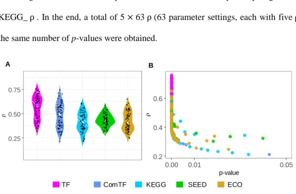
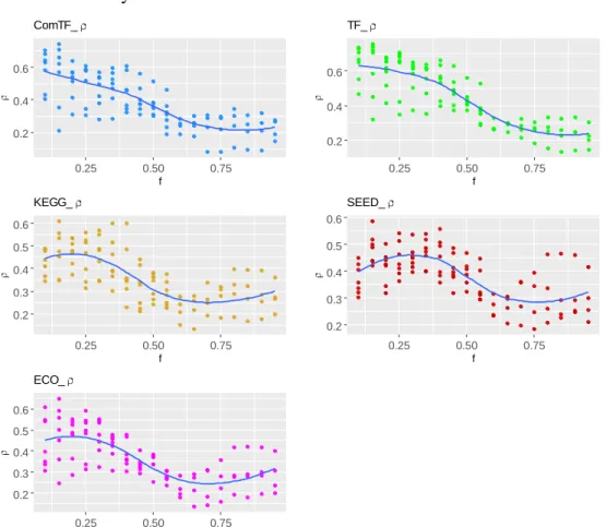
Figure 5.A. The distribution of correlation coefficients(ρ) between P-value obtained from enrichment analysis and size-based P-value.; B. Scatter plot of ρ and p-value.. ... 32 Figure 6. The relationship between biclustering parameter f and correlation coefficient. 33 Figure 7. A. Computational pipeline for cell type classification.; B. Benchmark of
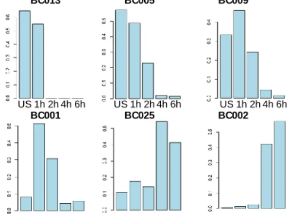
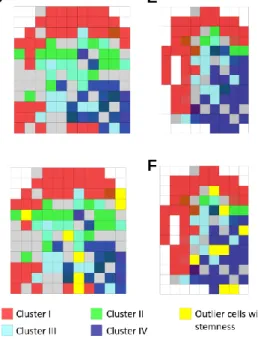
QUBIC2 against five popular biclustering algorithms; C. Sankey diagram. ... 39 Figure 8. A. Visualization of three biclusters (BC002, BC003, and BC004) selected based on the specificity to time point; B. Time-dependent distribution of cells in six selected biclusters identified in the LPS data.. ... 42 Figure 9. A. The coordinates of cells correspond to five morphological layers; B. The coordinates of cells from three selected biclusters; C. The spatial coordinates of samples in the four biclusters identified in wild-type 1 mouse; D. In addition to the coordinates of bicluster samples, the yellow cubes represent significant outlier samples; E. The same information as in C except the samples are from wild-type 2 mouse; F. The same
information as in D except the samples are from wild-type 2 mouse. ... 43 Figure 10. Performance of QUBIC2, QUBIC, two decomposition methods and two clustering methods in term of F score on a human scRNA-Seq data. ... 46
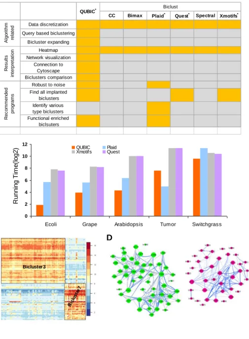
Figure 11. A. Comparison of QUBIC-R and 6 R packages in biclust; B. Comparison of running time among four recommended programs; C. Heatmap visualization of two biclusters identified in E. coli data; D. Co-expression networks of Figure 11C biclusters.
... 48
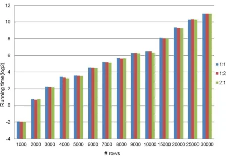
Figure 12. Data limit test of QUBICR on simulated datasets.. ... 50
Figure 13. Heatmap for the 4th bicluster identified in the E. coli data. ... 54
Figure 14. Network for the 4th bicluster identified in the E. coli data. ... 55
Figure 15. Yearly comparison of biclustering algorithm development and algorithm application related studies.. ... 60
Figure 16. The overall workflow of biclustering application mechanism related to upstream and downstream process... 82
LIST OF TABLES
Table 1. Summary of biclustering algorithms and tools, sorted in the decreasing order of
their numbers of citation since published ... 5
Table 2. Main parameter adjusted for each algorithm ... 26
Table 3. Parameter ranges for each biclustering algorithm used in the cell type classification section ... 35
Table 4. Summary of GSE60402 ... 40
Table 5. Case studies of Functional annotation of unclassified genes ... 63
Table 6. Case studies of Modularity analysis. ... 66
Table 7. Case studies of Biological networks elucidation. ... 70
Table 8. Case studies of disease subtype identification. ... 73
Table 9. Case studies of Biomarker and gene signatures detection. ... 77
Table 10. Case studies of gene-drug association. ... 79
ABSTRACT
DEVELOPMENT OF BICLUSTERING TECHNIQUES FOR GENE EXPRESSION DATA MODELING AND MINING
JUAN XIE
2018
The next-generation sequencing technologies can generate large-scale biological data with higher resolution, better accuracy, and lower technical variation than the array-based counterparts. RNA sequencing (RNA-Seq) can generate genome-scale gene expression data in biological samples at a given moment, facilitating a better
understanding of cell functions at genetic and cellular levels. The abundance of gene expression datasets provides an opportunity to identify genes with similar expression patterns across multiple conditions, i.e., co-expression gene modules (CEMs). Genome-scale identification of CEMs can be modeled and solved by biclustering, a
two-dimensional data mining technique that allows clustering of rows and columns in a gene expression matrix, simultaneously. Compared with traditional clustering that targets global patterns, biclustering can predict local patterns. This unique feature makes biclustering very useful when applied to big gene expression data since genes that participate in a cellular process are only active in specific conditions, thus are usually co-expressed under a subset of all conditions.
The combination of biclustering and large-scale gene expression data holds promising potential for condition-specific functional pathway/network analysis.
RNA-Seq data, majorly due to the lack of (i) a consideration of high sparsity of RNA-Seq data, especially for scRNA-Seq data, and (ii) an understanding of the underlying
transcriptional regulation signals of the observed gene expression values. QUBIC2, a novel biclustering algorithm, is designed for large-scale bulk RNA-Seq and single-cell RNA-seq (scRNA-Seq) data analysis. Critical novelties of the algorithm include (i) used a truncated model to handle the unreliable quantification of genes with low or moderate expression; (ii) adopted the Gaussian mixture distribution and an information-divergency objective function to capture shared transcriptional regulation signals among a set of genes; (iii) utilized a Dual strategy to expand the core biclusters, aiming to save dropouts from the background; and (iv) developed a statistical framework to evaluate the
significances of all the identified biclusters. Method validation on comprehensive data sets suggests that QUBIC2 had superior performance in functional modules detection and cell type classification. The applications of temporal and spatial data demonstrated that QUBIC2 could derive meaningful biological information from scRNA-Seq data.
Also presented in this dissertation is QUBICR. This R package is characterized by an 82% average improved efficiency compared to the source C code of QUBIC. It provides a set of comprehensive functions to facilitate biclustering-based biological studies, including the discretization of expression data, query-based biclustering, bicluster expanding, biclusters comparison, heatmap visualization of any identified biclusters, and co-expression networks elucidation.
In the end, a systematical summary is provided regarding the primary applications of biclustering for biological data and more advanced applications for biomedical data. It
will assist researchers to effectively analyze their big data and generate valuable biological knowledge and novel insights with higher efficiency.
CHAPTER 1: Introduction
1.1 Gene Expression Data
Gene expression is the process by which information from a gene is used in the synthesis of a functional product, that is, a molecule needed to perform a job in the cell (e.g., protein). The process mainly consists of two steps: transcription and translation. In transcription, the DNA sequence of a gene is copied to make an RNA molecule. In translation, the sequence of the mRNA is decoded to specify the amino acid sequence of a polypeptide. Since genes encode proteins and proteins dictate cell functions, the genes expressed in a cell determine what the cell can do.
Many biotechnologies are available to profile gene expression. Microarrays emerged in the late 1990s, which is the first high-throughput technology that enables the researchers to monitor the expression level of tens of thousands of genes simultaneously [1]. Microarrays are typically microscope slides that are printed with thousands of tiny spots in ordered positions, with each spot containing a known DNA sequence or gene. After steps of mRNA extraction, cDNA synthesis, cDNA fragmentation, and fluorescent labeling, the relative abundance of genes is quantified by detecting fluorescent intensity, which is continuous and positive. Due to its easy accessibility and low cost, microarrays have been the most widely used platforms in generating gene expression. However, microarrays need a reference genome and transcriptome to be available; thus, their application is confined to organisms whose genome have already been sequenced.
With the advent of massively parallel sequencing, next-generation sequencing (NGS) technologies have become more affordable. Compared to the array-based
counterparts, NGS has higher resolution, better accuracy, lower technical variation and many other advantages [2, 3]. It allows for a much faster-paced accumulation of large-scale biological data. The high-throughput RNA-sequencing (RNA-Seq) is a
revolutionary technology for gene expression profiling and promises a comprehensive picture of the transcriptome for a biological process [4, 5]. Unlike microarrays, RNA-Seq can be used to new organisms whose genome has not been sequenced yet. It extracts usable information from the mature mRNA within a biological source and generates a massive number of short segments (reads, 100-250 bps), which enable the discrete quantification of all genes expressed in a cell [5, 6]. Currently, researchers can either analyze a large sample of cells from a single organism in the form of bulk RNA-Seq data or isolate individual cells from complex organisms and measure their transactional activity through single-cell RNA-sequencing (scRNA-Seq). Such gene expression data from individual cells promises to provide a better understanding of cell functions at genetic and cellular levels[7] . In short, these biotechnologies have generated large genome-scale gene expression data in the public domain, and their tremendous values have been confirmed in many research areas such as elucidation of cell-type-specific regulatory networks [8, 9] and cancer & complex diseases studies [10-12].
1.2 Biclustering Techniques
The abundance of gene expression datasets provides an opportunity to identify genes with similar expression patterns across multiple conditions, i.e., co-expression gene modules (CEMs). The genes in these modules tend to be functionally related or co-regulated by the same transcriptional regulatory signals (TRSs). Thus, they enable the higher-level interpretation of gene expression data, improve functional annotation,
facilitate inference of gene regulatory mechanisms, and are useful for a better understanding of disease/cancer mechanisms. Genome-scale identification of CEMs can be modeled and solved by biclustering [13], which was introduced by Hartigan in 1972 [14] and applied to gene expression data analysis by Cheng and Church in 2000 [15]. Biclustering is a two-dimensional data mining technique that allows clustering of rows (representing genes) and columns (representing samples/conditions) in a gene expression matrix, simultaneously. The biclustering method can capture biologically meaningful and computationally significant CEMs, by identifying (possibly overlapped) homogeneous submatrices, subsets of rows with a coherent pattern across subsets of columns that satisfy specific quality metrics (e.g., mean squared residue used in [15] and MSE used in [16]). This unique feature makes it very useful when applied to big gene expression data since genes that participate in a cellular process are only active in specific conditions, thus are usually co-expressed under a subset of all conditions.
Besides the identification of CEMs, scRNA-Seq data enables studies of individual cells or cell types as well as their complex interactions under specific stimuli, e.g., cell types classification and clustering. In multicellular organisms, biological function emerges when various cell types form complex organs [17]. Investigations into organ development, cell function, and disease mechanisms highly depend upon accurate identification and categorization of cell types, sometimes along with their temporal and spatial features [18]. Traditionally, cell type was defined based on morphological properties or marker proteins, yet this method failed to characterize the full diversity of cells. scRNA-Seq data provides the possibility to group cells based on their genome-wide transcriptome profiles, and several studies have already been carried out using scRNA-Seq data to identify novel cell
types, proving its power to unravel the full diversity of cells in human and mouse [8]. Mathematically, the problem of cell types classification can be treated as biclustering problems, as the essence is to find sub-populations of cells sharing common expression patterns among subsets of genes.
A substantial number of biclustering methods were developed during the past 18 years [15, 16, 19-36]. SAMBA [28], ISA [29], Bimax [30], QUBIC [31], and FABIA [37] are some popular algorithms for general purpose. CCC-biclustering [38-40] is designed for temporal data analysis, and BicPAM [41], BicNET [35, 42] and MCbiclust [43] are three recent studies. Besides, several tools (R packages, web servers, etc.) have been developed to facilitate users with a limited computational background [23, 44-50]. GEMS [47] is a web server for gene expression mining based on a Gibbs sampling paradigm; and biclust [48] and QUBICR [49] are two R packages integrating multiple existing algorithms, data preprocessing functions, and interpretation & visualization of the results. A list of some highly cited or recently published biclustering algorithms and tools is shown in Table1.
Table 1. Summary of biclustering algorithms and tools, sorted in the decreasing order of their numbers of citation since published. Application or usage was noted for some of the algorithms. Citations were collected via Google Scholar as of Sep 2018
Algorithms/ Tools
Citations* Published Year
Review comments* Notes
SAMBA [28] 939 2002 - -
Bimax[30] 874 2006 E Choice for constant-upregulated biclusters -
ISA [29] 414 2002 E Choice for constant-upregulated biclusters;
NC Performs well on synthetic data
-
Plaid[16] 717 2002 E Choice for constant-upregulated biclusters;
Has the highest enriched bicluster ratio in real datasets
Spectral[51] 654 2003 NC Performs well on human and synthetic
data cMonkey[52] / cMonkey2 [53] 257/ 21 2006/ 2015
- Integrates various orthogonal pieces
of information which support evidence of gene co-regulation, and optimizes biclusters to be supported simultaneously by one or more of these prior constraints
FABIA [32] 198 2010 E Choice for constant-upregulated biclusters;
NC Performs well on synthetic data
-
QUBIC [31] 167 2009 E Choice for constant-upregulated
biclusters; Has the highest enriched bicluster ratio in real datasets
NC Performs well on synthetic and human
data
BBC[55] 126 2008 E Best one for plaid biclusters -
CPB[56] 40 2009 E Best one for constant, scale, shift and
shift-scale datasets
LAS [57] 113 2009 - Discovery of biologically relevant
structures in high dimensional data; Significant results highlighted with a large negative average image for easy observation.
BackSPIN [58] 830 2015 - First biclustering algorithm for
scRNA-Seq data
PPA [59] 93 2008 - -
CCC-Biclustering [60] 95 2010 - Coherent biclusters with maximal
contiguous columns in linear time; Combining time-series expression with the regulatory network.
COALESCE [61] 80 2009 E Choice for constant-upregulated biclusters Efficient enough to discover
expression biclusters and putative regulatory motifs in metazoan genomes and very large microarray compendia (>10,000 conditions)
BioNMF [62] 79 2006 - -
Note: In the Reviewer Comments column, algorithms/tools mentioned by [69] are denoted by ‘E’, mentioned by [70] are denoted by ‘NC’
NCIS [63] 44 2014 - Identification of cancer subtypes
FD-MSCM [64] 35 2010 - -
BicPAM [41] 28 2014 - Biclustering for biomedical data
analysis;
Suitable for non-constant biclusters
IBBiG [65] 24 2012 - -
BUBBLE [66] 14 2006 - Based on bottom-up search strategy;
Using mean squared residue measurement.
SparseBC [67] 21 2014 - -
BicNET [35] 13 2016 - Discovery of non-trivial modules
directly for biological network construction;
Noisy and missing interaction fix; Analysis of protein interaction and gene interaction networks
Several review studies of biclustering have been carried out in different perspectives [30, 71-75]. For example, Pontes et al. presented a taxonomy of 47
biclustering algorithms according to their search strategies [76], and Busygin et al.
emphasized the mathematical models and concepts in biclustering techniques [77]. Padilha et al. claimed that an algorithm only achieved satisfactory results in a specific context and
the best choice depends on particular objectives [74]. Eren et al. compared 12 popular
algorithms and concluded that QUBIC is one of the best as it achieves the highest performance in synthetic datasets and captures a high proportion of enriched biclusters on real datasets, and Plaid, FABIA, ISA and Bimax are the recommended tools for capturing upregulated biclusters [78]. Adetayo et al. presented an overview of data analysis using
biclustering methods from a practical point of view, accompanied by R examples [79].In 2018, Saelens et al. ranked Spectral, ISA, FABIA and QUBIC as the top biclustering
methods regarding predicting gene modules from human and/or synthetic data [70].
1.3 QUBIC
QUBIC (Qualitative BIClustering algorithm) is a qualitative biclustering algorithm, which was first introduced in 2009. It assumes that a gene has three
expression states under all the conditions, i.e., highly-expressed, lowly-expressed, and normally-expressed. The values in the first two expression states are so-called affected values. QUBIC employs a framework to identify dynamic cutoffs and corresponding affected values for different genes (Figure 1). A discretized qualitative matrix (MR) can
be generated after applying the above process to each gene, with non-zero integers representing affected values and 0s being background. Then a weighted graph is
has a weight indicating the similarity level between the two corresponding genes. The aim is to search biclusters corresponding to induced heavy subgraphs, which is an NP-hard problem. QUBIC heuristically iterates a seed list (S), where a seed represents a pair of genes, and its weight is the number of conditions under which they have the same values in MR. In each iteration, it starts from a feasible seed with the highest weight, then
expands vertically and horizontally to recruit more genes and conditions. Finally, QUBIC outputs a bicluster with max (min (I, J)), where I and J being the number of rows and columns of the bicluster (Figure 1).
1 … 1 … -1 … -1 … 1 1 … 1 … -1 … -1 … 1 7.6 6.0 7.3 8.3 9.1 8.7 7.4 6.4 9.2 6.5 8.1 7.2 8.4 8.9 8.8 6.5 1 -1 0 1 1 1 0 0 1 -1 1 0 1 1 1 -1 1 … 1 … -1 … -1 … 1 1 … 1 … -1 … -1 … 1 1 … 1 … -1 … -1 … 0 1 … 1 … -1 … -1 … 1 1 … 1 … -1 … -1 … 1 1 … 1 … -1 … -1 … 0 1 … 1 … -1 … -1 … 0 min{I,J}=2 min{I,J}=3 min{I,J}=4 Reach max(min(I,J)), Output M L U’ U -1 0 1 C1 C2 C3 C4 C5 C6 C7 C8 C9C10C11C12C13C14C15C16 G1 1 -1 0 1 1 1 0 0 1 -1 1 0 1 1 1 -1 G2 1 -1 1 1 1 1 0 1 1 0 1 -1 1 0 1 0 … 1 0 1 0 -1 1 -1 1 0 1 1 -1 1 0 1 1 U’- M = M- L
Figure 1. Workflow of QUBIC. QUBIC sorts the expression values of the gene i under all given conditions in an increasing order: 𝑣𝑖1⋯ 𝑣𝑖,𝑠−1𝑣𝑖𝑠⋯ 𝑣𝑖,𝑐−1𝑣𝑖𝑐𝑣𝑖,𝑐+1⋯ 𝑣𝑖,𝑚−𝑠+1𝑣𝑖,𝑚−𝑠+2⋯ 𝑣𝑖𝑚 , where c=m/2 and s-1= m×q (q=6% by default). Then it selects initial bounds L= 𝑣𝑖,𝑠−1and U= 𝑣𝑖,𝑚−𝑠+1. QUBIC adjusts the bounds based on their distance from the median (M= 𝑣𝑖𝑐), e.g., if (U-M) > (M-L), then use U’ = (M-L) + M = 2M –L as the new upper bound. The values less or equal to L are labeled as -1, those greater or equal to U’ are labeled as 1, and those fall between L and U’ are labeled as 0. Repeat this process for each gene in the dataset, a representing matrix MR
can be generated.
1.4 Qserver
QUBIC has been proved to be able to solve more general biclustering problems than previous biclustering algorithms[31]. To fully utilize the analysis power of QUBIC, a web server named Qserver (Qualitative BIClustering server) was developed in
2011[23]. Qserver integrates capabilities of biclustering with cis-regulatory motifs
prediction and functional enrichment analyses. Specifically, Qserver provides the following functionalities: (i) biclustering analysis using QUBIC; (ii) prediction and assessment of conserved cis-regulatory motifs in promoter sequences of the predicted co-expressed genes; (iii) functional enrichment analyses of the predicted co-co-expressed gene clusters using Gene Ontology (GO) terms, and (iv) visualization capabilities in support of interactive biclustering analyses.
For biclustering analysis, QUBIC algorithm is implemented. Users can provide continuous or discretized gene expression matrix as input. If continuous data is provided, Qserver will automatically discretize it qualitatively. Qserver allows users to adjust the main parameters in QUBIC, and suggestion regarding how to change for different applications is provided in the Help page.
After obtaining sets of biclusters, QServer allows computationally validating of the biclusters by predicting conserved cis-regulatory motifs among the promoter
sequences automatically extracted from the upstream sequences (the default value is 300 bps long) of the co-expressed genes. Two motif prediction programs, BOBRO [80] and MEME[81] are provided, both of which attempt to find conserved sequences among a set of given promoter sequences using different strategies, and both offer a statistical significance score for each predicted motif.
For the predicted biclusters, Qserver can also conduct functional enrichment analysis based on GO classification. Specifically, given a bicluster, Qserver will check if it is enriched with a GO term, compared against the background gene distribution, i.e., the whole genome. A P-value and enrichment ratio of that GO term will be provided.
It is common that different sets of gene expression data may use different naming conventions for genes. To deal with this issue, Qserver collected three gene/protein naming systems (i.e., GI, locus, and RefSeq) so that it can automatically detect the naming system used in an expression matrix. It also collected the genome sequences and the gene annotations from the NCBI Genome database in support of motif prediction and functional enrichment analysis, covering human, mouse, Arabidopsis, B subtilis,
Synechocystis sp. PCC6803, Synechococcus sp. WH8102 and E. coli K12. For other
organisms, Qserver will only do biclustering analysis and plot the heatmaps for biclusters.
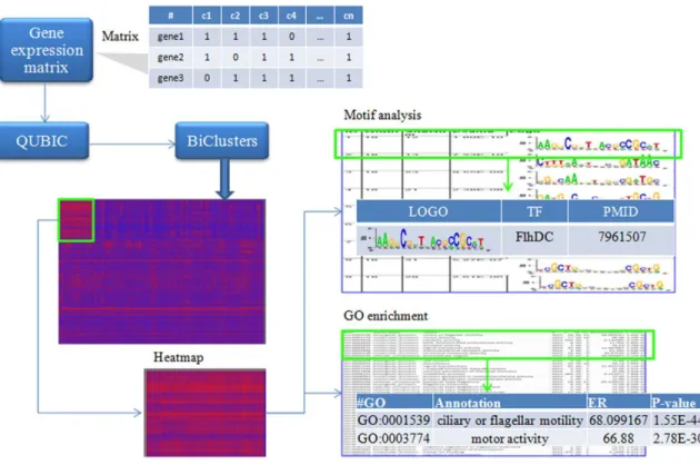
In summary, Qserver provides three functional modules for the expression data. First, the input matrix is subject to biclustering analysis using QUBIC. For each bicluster, cis-regulatory motifs are then identified in the promoter regions of its
component genes, using either MEME or BOBRO. Qserver will also provide the detailed information of each identified motif, including its P-value and the logo plot. The third module is to identify enriched GO categories among genes in each bicluster. The workflow of Qserver is shown in Figure 2.
Figure 2. An example workflow of using Qserver.
CHAPTER 2: QUBIC2—A Novel Biclustering Algorithm for Large-scale RNA-Seq Data Analysis
Although numerous algorithms and tools have been developed for gene expression data analysis, most existing biclustering algorithms are designed and
evaluated using microarray rather than RNA-Seq data. One of the unique features of gene expression data derived from RNA-Seq, especially the scRNA-Seq data, is the massive zeros (up to 60% of all the genes in a cell have read counts being zeros) [82, 83]. The normalized read counts roughly follow lognormal distributions; however, the raw zero counts of specific genes will lead to negative infinity after logarithmic transformation [84-87], resulting in unquantifiable errors. Therefore, the biclustering methods that are successful for microarray cannot be directly applicable to RNA-Seq data [88], and novel methods taking full consideration of characteristics of RNA-Seq data are urgently needed in the public domain. In this chapter, I will present QUBIC2, a novel biclustering
algorithm developed for large-scale RNA-Seq data analysis.
2.1 Overall Design of QUBIC2
Inheriting the qualitative representation and graph-theory based model from QUBIC [31], QUBIC2 has four unique features: (i) developed a rigorous truncated model
to handle the unquantifiable errors caused by zeros, and useda reliable qualitative representation of gene expression to reflect expression states corresponding to various TRSs; (ii) integrated an information-divergence objective function in the biclustering
framework in support of functional gene modules identification; (iii) employed a Dual
developed a robust P-value framework to support statistical evaluation of all the
identified biclusters. Details of these four features are showcased as follows.
A mixture of left-truncated Gaussian distributions (LTMG) model was designed to fit the RNA-Seq data, rather than discarding zeros or adding a small constant to original counts [85, 89]. The basic idea is to treat the large number of observed zeros and low expressions as left censored data in the mixture Gaussian model of each gene [90, 91], assuming that the observed frequency of expressions on the left of the censoring point should be equal to the area of the cumulative distribution function of the mixture Gaussian distribution left of the censoring point. Furthermore, we assumed that a gene should receive 𝐾 possible TRSs under all the conditions, and its expression profile would follow a mixture of 𝐾 left truncated Gaussian distributions. The LTMG model was applied to fit the expression value of each gene, and the gene expression value under a specific condition was labeled to the most likely distribution. Accordingly, a row consisting of discrete values (1,2, ⋯, 𝐾) for each gene was generated (Figure 3A). Then this qualitative row was split into 𝐾 new rows, such that in the 𝑖th row those previously labeled as 𝑖 are labeled as 1,
while the rest were labeled as 0. Finally, a binary representing matrix MR was generated.
A weighted graph 𝐺 = (𝑉, 𝐸) was constructed based on MR, where nodes 𝑉
correspond to genes, edges 𝐸 connecting every pair of genes (Figure 3B). The edge weight indicates the similarity between the two corresponding genes, which is defined as the number of conditions in which the two genes have 1s in MR. Intuitively, two genes from a
bicluster should have a heavy edge in 𝐺 innately while two random genes may have a heavy edge only accidentally. Hence, a bicluster should correspond to a maximal subgraph of 𝐺, with edges typically heavier than the edges of an arbitrary subgraph. Identifying all
the biclusters equals to identifying all the heavy subgraphs in 𝐺, which is an NP-hard problem. Therefore, a heuristic strategy was designed as follows.
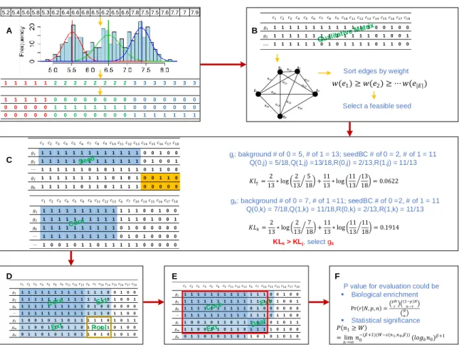
Figure 3. QUBIC2 workflow. A. Discretization of gene expression data. Each gene’s expression profile is fitted by the LTMG model and discretized qualitatively. Finally, a binary representing matrix is generated; B. Graph construction and seed selection. A weighted group is constructed based on the representing matrix. Then a feasible seed is selected from the seed list; C. Build an initial core based on the seed. QUBIC2 will recruit genes with higher weight with the seed. If two genes have the same weight, the one with higher KL score will be selected; D. Expand core and determine pool. QUBIC2 will expand the core vertically and horizontally to recruit more genes and conditions, respectively. The intersected zone created by extended genes and conditions as a Dual searching pool; E. Dual search in the pool and output the bicluster with genes and
conditions that come from Core and Dual as final bicluster (red box); F. Statisticalevaluation of identified biclusters based on either biological annotations or the size of the bicluster.
1 2 1 11121 1 1 1 1 1 1 1 1 1 1 1 1 1 1 1 1 1 1 1 0 0 1 0 0 2 1 1 1 1 1 1 1 1 1 1 1 1 1 0 1 0 0 1 ⋯ 1 1 1 1 1 1 0 1 0 1 1 1 1 0 1 1 0 0 1 1 1 1 1 1 1 1 1 0 1 0 1 0 0 1 1 0 1 1 1 1 1 0 1 1 0 1 1 1 1 0 0 0 0 0 gj: bakground # of 0 = 5, # of 1 = 13; seedBC # of 0 = 2, # of 1 = 11 Q(0,j) = 5/18,Q(1,j) =13/18,R(0,j) = 2/13,R(1,j) = 11/13 gk: background # of 0 = 7, # of 1 =11; seedBC # of 0 =2, # of 1 = 11 Q(0,k) = 7/18,Q(1,k) = 11/18,R(0,k) = 2/13,R(1,k) = 11/13 KLk > KLj, select gk A B C D E F Pr(𝑟 𝑁,𝑝,𝑛)= 𝑝𝑁 𝑟 (1𝑛−𝑟−𝑝)𝑁 𝑁 𝑛 𝑃(𝑛1≥ 𝑊) = lim 𝑛→∞𝑛0 −(𝛽+1)(𝑊−𝑠(𝑛1,𝑛0,𝛽))(𝑙𝑜 𝑏𝑛0)𝛽+1
P value for evaluation could be
▪ Statistical significance ▪ Biological enrichment 𝐾𝐿𝑗=132∗log 132 185 +1113∗log 1113 1318 = 0.0622 𝐾𝐿𝑘=132∗log 132 187 +1113∗log 1113 1118 = 0.1914 g1 g2 g3 g4 gn e12 e13 e14 e23 e34 e24 e2n e1n e3n e4n
Sort edges by weight
Select a feasible seed 𝑤(𝑒1)≥ 𝑤(𝑒2)≥ ⋯ 𝑤(𝑒|𝐸|) 1 2 1 11121 1 1 1 1 1 1 1 1 1 1 1 1 1 1 1 1 1 1 1 0 0 1 0 0 2 1 1 1 1 1 1 1 1 1 1 1 1 1 0 1 0 0 1 ⋯ 1 1 1 1 1 1 0 1 0 1 1 1 1 0 1 1 0 0 1 2 11121 1 1 1 1 1 1 1 1 1 1 1 1 1 1 1 1 1 1 1 1 0 0 1 0 0 2 1 1 1 1 1 1 1 1 1 1 1 1 1 0 1 0 0 1 1 1 1 1 1 1 1 1 1 1 0 1 0 0 0 0 0 0 ⋯ 1 1 1 1 1 1 1 1 1 1 0 1 0 1 0 0 0 0 ⋯ 1 0 0 1 0 1 1 0 1 1 1 1 1 0 0 0 0 0 1 2 11121 1 1 1 1 1 1 1 1 1 1 1 1 1 1 1 1 1 1 1 1 0 0 1 0 0 2 1 1 1 1 1 1 1 1 1 1 1 1 1 0 1 0 0 1 1 1 1 1 1 1 1 1 1 1 0 1 0 0 0 0 0 0 ⋯ 1 1 1 1 1 1 1 1 1 1 1 1 1 0 1 1 0 0 1 0 0 1 0 1 1 0 1 1 1 1 1 0 1 0 1 1 𝑚 1 1 0 0 1 1 0 1 1 0 1 1 1 1 0 1 0 0 0 1 1 0 1 0 1 1 0 1 1 0 1 0 1 0 1 0 1 2 11121 1 1 1 1 1 1 1 1 1 1 1 1 1 1 1 1 1 1 1 1 0 0 1 0 0 2 1 1 1 1 1 1 1 1 1 1 1 1 1 0 1 0 0 1 1 1 1 1 1 1 1 1 1 1 0 1 0 0 0 0 0 0 ⋯ 1 1 1 1 1 1 1 1 1 1 1 1 1 0 1 1 0 0 1 0 0 1 0 1 1 0 1 1 1 1 1 0 1 0 1 1 𝑚 1 1 0 0 1 1 0 1 1 0 1 1 1 1 0 1 0 0 0 1 1 0 1 0 1 1 0 1 1 0 1 0 1 0 1 0 5.2 5.4 5.6 5.8 5.3 6.2 6.4 6.6 6.8 6.5 6.2 6.5 6.6 7.8 7.5 7.5 7.6 7.7 7 7.9 1 1 1 1 1 2 2 2 2 2 2 2 2 3 3 3 3 3 3 3 1 1 1 1 1 0 0 0 0 0 0 0 0 0 0 0 0 0 0 0 0 0 0 0 0 1 1 1 1 1 1 1 1 0 0 0 0 0 0 0 0 0 0 0 0 0 0 0 0 0 0 0 0 1 1 1 1 1 1 1 Pool
The algorithm would iterate a seed list (𝑆), which is the sorted list of edges in 𝐺 in the decreasing order of their weights (i.e., 𝑤(𝑒1) ≥ 𝑤(𝑒2) ≥ ⋯ , 𝑤(𝑒 𝐸 ) ). An edge 𝑒𝑖 =
𝑖 is selected as a seed if and only if at least one of 𝑖 and is not in any previously identified biclusters, or 𝑖 and are in two nonintersecting biclusters in terms of genes. QUBIC2 first built a core bicluster from a seed and then expanded to recruit more genes and conditions into a to-be-identified bicluster, until the Kullback-Leibler divergence score (KL score) was locally optimized. It was proposed based on the assumption that the difference between a bicluster and its background should be larger than the difference between an arbitrary same-size submatrix and its background. The KL score of a bicluster was designed to quantify this difference as the larger of the difference was, the larger of the score is (Figure 3C. See Section 2.2.2 for details).
The previous steps predict an all-1 core. We believe that some 0s outside the cores are dropouts and therefore we need to expand the cores. Since it is difficult to determine the cutoffs for expansion, we first expand the core both horizontally and vertically, and then heuristically search another core in the expanded region. Specifically, during expansion, the algorithm will control the consistency level for a bicluster, which is defined as the minimum ratio of the number of 1s in a column/row and the number of rows/columns in the bicluster. Then QUBIC2 will adopt the same strategy as it used for predicting Cores to search another core in the expanded region (Figure 3D-E), giving rise to a submatrix (I, J) of MR (i.e., a bicluster) with optimized consistency level and maximal KL score can be
identified. It is assumed that 0s induced in this way are more likely to be dropouts.
Furthermore, for the first time, a statistical framework based on the size of the biclusters was implemented to calculate a P-value for each of the identified biclusters. The
problem of assessing the significance of identified biclusters was formulated as calculating the probability of finding at least one submatrix enriched by 1 from a binary matrix with given size, with a beta distribution employed during the process. This P-value framework
enables users systematically evaluate the statistical significance of all the identified biclusters, especially for those from less-annotated organisms (Figure 3F).
2.2 Detailed Methods in QUBIC2
2.2.1 Left Truncated Mixed Gaussian (LTMG) Model and Qualitative Representation To accurately model the gene expression profile of RNA-Seq and scRNA-Seq data, we explicitly developed a mixed Gaussian model with left truncation assumption. Denotes the log-transformed FPKM, RPKM or CPM expression values of gene X over 𝑁 conditions as X = {𝑥1,𝑥 }, we assumed that 𝑥 𝑋 follows a mixture of 𝑘 Gaussian distributions, corresponding to 𝑘 possible TRSs. The density function of 𝑥 is:
𝑝 𝑥; Θ = ∑ 𝛼𝑖𝑝(𝑥; 𝜃𝑖) 𝑖=1 = ∑ 𝛼𝑖 1 √2𝜋𝜎𝑖 𝑒 − 𝑥𝑗−𝜇𝑖 2 2𝜎𝑖2 𝑖=1
And the density function of X is:
𝑝(X; Θ) = ∏ 𝑝(𝑥 ; Θ) =1 = ∏ ∑ 𝛼𝑖𝑝(𝑥; 𝜃𝑖) 𝑖=1 =1 = ∏ ∑ 𝛼𝑖 1 √2𝜋𝜎𝑖 𝑒 − 𝑥𝑗−𝜇𝑖 2 2𝜎𝑖2 𝑖=1 =1 = 𝐿(Θ; 𝑋)
where 𝛼𝑖 is the mixing weight, 𝜇𝑖 and 𝜎𝑖 are the mean and standard deviation of ith
Gaussian distribution, which can be estimated by the EM algorithm with given X: Θ∗ =
Θ
arg max 𝐿(Θ;𝑋)
To model the errors at zero and the low expression values, we introduce a parameter 𝑍𝑐𝑢𝑡 for each gene expression profile and consider the expression values
smaller than 𝑍𝑐𝑢𝑡 as left censored data. With the left truncation assumption, the gene expression profile is split into 𝑀 truly measured expression value (> 𝑍𝑐𝑢𝑡) and 𝑁 − 𝑀 left censored gene expressions (≤𝑍𝑐𝑢𝑡) for the 𝑁 conditions. Latent variables 𝑦 and 𝑍 are introduced to estimate Θ by the following Q function:
𝑄(Θ; Θ𝑡−1) = ∑ 𝑝 𝑦|𝑥; 𝛩𝑡−1 ∑ ∑ log (𝛼 𝑖𝑝(𝑥; 𝜇𝑖, 𝜎𝑖) 𝑖=1 ) 𝑚 =1 + ∑ 𝑝 𝑦|𝑧; 𝛩𝑡−1 ∑ ∑ log (𝛼 𝑖𝑝(𝑧; 𝜇𝑖, 𝜎𝑖) 𝑖=1 ) =𝑚+1
To estimate the parameters Θ that maximizes the likelihood function, we have Maximization step of the EM algorithm as [92]:
𝑎𝑖𝑡 = 1 𝑁(∑ 𝑃 𝑖|𝑥, Θ𝑡−1 𝑀 =1 + ∑ 𝑃(𝑖 𝑍, 𝑍𝑐𝑢𝑡, Θ𝑡−1)) 𝑁 =𝑀+1 𝑢𝑖𝑡 =∑ 𝑥𝑃 𝑖|𝑥, Θ 𝑡−1 + ∑ (𝑢 𝑖 𝑡−1− 𝜎 𝑖𝑡−1𝐻(𝑍𝑐𝑢𝑡− 𝑢𝑖 𝑡−1 𝜎𝑖 ))𝑃(𝑖 𝑍, 𝑍𝑐𝑢𝑡, Θ𝑡−1) 𝑁 =𝑀+1 𝑀 =1 ∑𝑀 𝑃(𝑖 𝑥, Θ𝑡−1) =1 + ∑𝑁 =𝑀+1𝑃(𝑖 𝑍, 𝑍𝑐𝑢𝑡, Θ𝑡−1) 𝜎𝑖𝑡2 =∑ 𝑃 𝑖|𝑥, Θ 𝑡−1 (𝑥 − 𝑢 𝑖𝑡−1)2+ 𝜎𝑖𝑡−1 2 ∑ (1 −𝑍𝑐𝑢𝑡− 𝑢𝑖𝑡−1 𝜎𝑖 ∗ 𝐻( 𝑍𝑐𝑢𝑡− 𝑢𝑖𝑡−1 𝜎𝑖 )) ∗ 𝑃(𝑖 𝑍, 𝑍𝑐𝑢𝑡, Θ 𝑡−1) 𝑁 =𝑀+1 𝑀 =1 ∑𝑀 𝑃(𝑖 𝑥 , Θ𝑡−1) =1 + ∑𝑁 =𝑀+1𝑃(𝑖 𝑍, 𝑍𝑐𝑢𝑡, Θ𝑡−1) where 𝑃 𝑖|𝑍, 𝑍𝑐𝑢𝑡, Θ𝑡−1 = 𝑃(−∞<𝑍𝑗<𝑍𝑐𝑢𝑡 𝑢𝑖 𝑡−1,𝜎 𝑖𝑡−1) ∑𝐾𝑖=1𝑃(−∞<𝑍𝑗<𝑍𝑐𝑢𝑡 𝑢𝑖𝑡−1,𝜎𝑖𝑡−1), 𝐻(𝑥) = 𝜙(𝑥) Φ(𝑥), 𝜙(𝑥) and Φ(𝑥) are the pdf and cdf of standard normal distribution.
Parameters Θ can be estimated by iteratively running the estimation (E) and maximization (M) steps. In this study, 𝑍𝑐𝑢𝑡 is set for each gene as the logarithm of the minimal non-zero RPKM/FPKM/TPM value in the gene’s expression profile. The EM
algorithm is conducted for 𝐾 = 1, …, 9 to fit the expression profile of each gene and the 𝐾 that gives the best fit is selected according to the Bayesian Information Criterion (BIC):
𝐵𝐼𝐶 = −2 ln(Θ∗) + 3𝐾ln(𝑁)
where 𝐾 is the number of TRS, 𝐾 is the number of conditions. 𝐾 that minimizes the BIC will be selected.
Then the original gene expression values will be labeled to the most likely distribution under each condition. In detail, the probability that 𝑥 belongs to distribution 𝑖 is formulated by: 𝑝 𝑥 ∈ 𝑇𝑅𝑆 𝑖|𝐾, Θ∗ ∝ 𝛼𝑖 √2𝜋𝜎2 𝑒 −(𝑥𝑗−𝜇𝑖)2 2𝜎𝑖2 And 𝑥 is labeled by TRS 𝑖 if 𝑝 𝑥 ∈ 𝑇𝑅𝑆 𝑖|𝐾, Θ∗ = max 𝑖=1,⋯,𝐾(𝑝 𝑥 ∈ 𝑇𝑅𝑆 𝑖|𝐾, 𝛩
∗ ). In such a way, a row consisting of discrete values (1,2,
, 𝐾) for each gene will be generated. 2.2.2 KL Score
A Kullback-Leibler divergence score (KL score) is introduced in QUBIC 2 to guide candidate-selection and biclustering optimization. The KL score of a bicluster is defined as: 𝐾𝐿𝐵 = 1 𝑁∑ ∑ 𝑅(𝑖, 𝑗) × 𝑙𝑜 𝑅(𝑖, 𝑗) 𝑄(𝑖, 𝑗)+ 1 𝑀 𝑖∈{ ,1} 𝑁 =1 ∑ ∑ 𝐶(𝑖, 𝑘) × 𝑙𝑜 𝐶(𝑖, 𝑘) 𝑃(𝑖, 𝑘) 𝑖∈{ ,1} 𝑀 =1
where 𝑁 and 𝑀 are the numbers of rows and columns of a submatrix B in MR, respectively.
𝑅(𝑖, 𝑗) represents the proportion of element 𝑖 in row 𝑗 of B, 𝑄(𝑖, 𝑗) is the proportion of 𝑖 in the entire corresponding row, 𝐶(𝑖, 𝑘) is the proportion of 𝑖 in column 𝑘 of B, and 𝑃(𝑖, 𝑘) is the proportion of 𝑖 in the entire corresponding column.
Meanwhile, the KL score for a gene quantify the similarity between a candidate gene 𝑗 and a bicluster, which is defined as follows:
𝐾𝐿 = ∑ 𝑅(𝑖, 𝑗) × 𝑙𝑜 𝑅(𝑖, 𝑗) 𝑄(𝑖, 𝑗) 𝑖∈{ ,1}
where 𝑅(𝑖, 𝑗) represent the proportion of 𝑖 under corresponding columns of the current bicluster.
2.2.3 QUBIC2 Algorithm
TheQUBIC2algorithmconcludes as follows:
Step 1 (Data discretization and qualitative representation): Given an expression matrix with log-transformed FPKM, RPKM or CPM value for genes, use LTMG model to fit data. Label the values to the most likely distribution to get a representing row for each gene. Split these rows into multiple rows to get the representative matrix MR (Figure 3A).
Step 2 (Graph construction and seed selection): Construct a weighted graph for MR. Select a feasible seed from the seed list; Stop if the seed list is empty (Figure 3B).
Step 3 (Build core bicluster): Build an initial bicluster by finding all the conditions under which the two genes of the seed have 1s in MR. Set these columns of the two genes
as the current bicluster B = (I, J). Expand B by adding a new gene that has the most 1s in
J, giving rise to a new bicluster B’ = (I’, J’), where I’ is I after adding the new gene and J’ is J by deleting those columns with 0s. If two genes have the same number of 1s in J,
choose the one with larger KL similarity with B(Figure 3C). If KLB’ > KLB, set B to B’
Step 4 (Core expansion): Expand the Core horizontally and vertically under preset consistency level as follows: for each gene(row) i not in B, if the ratio between the number of 1s in row i under J and |J| is ≥c, mark it as an extended gene; for each condition (column) j not in B, if the ratio between the number of 1s in the column j among I and |I| is ≥c, mark it as an extended condition. (Figure 3D). Mark the intersected zone created by extended genes and conditions as a Dual searching pool (brown box in Figure 3D). Go to Step 5.
Step 5 (Search Dual): Search Dual in the intersected expanded zone, using the same process in Step 3, output the bicluster with genes and conditions that come from Core and Dual (red box in Figure 3E). Delete current seed, go to step 1.
2.2.4 Size-based P-value
For well-annotated organisms, the P-value of an identified bicluster enriching
with a specific regulatory pathway can be calculated based on a hypergeometric
distribution. However, the known experimental annotation is currently limited, even for most well-studied model organisms (about half of the protein-coding genes of E. coli
have solid experimental evidence for their function in KEGG and GO) [93]. This status still limits the capability of a systematic evaluation of all the identified biclusters. To fill this gap, we calculate an alternative size-based P-value as follows. For a binary
representing matrix MR,containing 𝑚 rows and 𝑛 columns, suppose we obtain an 𝑚1 -by-𝑛1bicluster M1 with all the elements be 1s. The probability of 𝑛1 ≥ 𝑊 can be assessed
by the following formula [94], giving rise to a P-value of the bicluster M1:
𝑃(𝑛1≥ 𝑊) = lim →∞𝑛 −(𝛽+1) 𝑊−𝑠( 1, 0,𝛽) (log 𝑏𝑛 )𝛽+1 where𝛼 =𝑚0 0 , 𝛽 = 𝑚1 1 , 𝑏 = 1 𝑝, 𝑝 = 𝑃 𝑀𝑖, = 1 = 1 − 𝑃 𝑀𝑖, = 0 for ∀𝑖, 𝑗
𝑠(𝑛1, 𝑛 , 𝛽) = 𝛽 + 1 𝛽 log𝑏𝑛 − 𝛽 + 1 𝛽 log𝑏 𝛽 + 1 𝛽 log𝑏𝑛 + log𝑏𝛼 +(1 + 𝛽) log𝑏𝑒 − 𝛽 log𝑏𝛽 𝛽
2.3 Functional Gene Modules Detection from RNA-Seq Data
2.3.1 Data Acquisition
A total of four expression datasets were used in this section, that is, one synthetic RNA-Seq data (22,846 rows × 100 columns), one bulk RNA-Seq dataset from
Escherichia coli (E. coli, 4,497 rows × 155 columns), a bulk RNA-Seq dataset from TCGA (3,084 rows × 8,555 columns), and a scRNA-Seq dataset from human embryos (3,798 genes × 90 cells). The synthetic dataset was simulated using our in-house
simulation method (see Section 2.3.2). It contains 22,846 genes and 100 samples. A total of 10 co-regulated modules was embedded in this dataset, covering 2,240 up-regulated genes. The E. coli RNA-Seq data consists of 4,497 genes and 155 samples, which was
integrated and aggregated by our group. In short, 155 fastq files were downloaded from ftp://ftp.sra.ebi.ac.uk/vol1/fastq/ using the sratoolkit (v2.8.1,
https://github.com/ncbi/sra-tools/wiki/Downloads), and they are processed following quality check (FastQC), reads trimming (Btrim), reads mapping (HISAT2) and transcript counting (HTSeq). Then, raw read counts were RPKM normalized. The human RNA-Seq data contains 3,084 genes and 8,555 samples, which was obtained from [70]. The scRNA-Seq data was downloaded from [95] as an RPKM expression matrix with 20,214 gene and 90 cells, and then 3,798 genes were kept for the analysis in this study by removing the genes without annotation.
Multiple sets of known modules/biological pathways were provided or collected to support the enrichment analysis of the above four datasets. For synthetic data, the ten
groups of pre-defined up-regulated genes were used as co-regulated modules. For E. coli
data, we used five kinds of biological pathways, which are complex regulons and regulons extracted from the RegulonDB database (version 9.4, accessed on 05/08/2017), KEGG pathways collected from the KEGG database (accessed on 08/08/2017), SEED subsystems from the SEED genomic database (accessed on 08/08/2017) [96], and EcoCyc pathways from the EcoCyc database (version 21.1, as of 08/08/2017) [97]. Complex regulons (ComTF) were defined as a group of genes that are regulated by the same transcription factor (TF) or the same set of TFs. In total, 457 complex regulons, 204 regulons, 123 KEGG pathways, 316 SEED subsystems, and 424 EcoCyc pathways were retrieved, respectively. For the human TCGA and scRNA-Seq data, we used three sets of modules provided by [70].
2.3.2 Simulation of Co-regulated Gene Expression Data
We utilized a single cell RNA-Seq dataset of human melanoma [98] (with 22,846 genes and 4,645 cells) to simulate bulk tissue RNA-Seq data with known co-regulated modules. Specifically, a single cell RNA-Seq pool consists counts data of 4,466 cells of six annotated cell types namely B-, T-, endothelial, fibroblast, macrophage, and cancer cells were constructed. The top 1,000 cell type specifically expressed genes of each cell type were identified by using Z score of the mean of each gene’s expression level in each cell type.
For each round of simulation, the number of to be simulated bulk tissue samples and co-regulation modules is first defined. Then the genes of each co-regulation module denoted as 𝑋 will be specified by randomly selecting 𝑀 genes from the top 1,000 cell type specifically expressed genes of one cell type. A co-regulation strength matrix 𝑃 is then
simulated from a bimodal distribution over (0,1), with 𝑃[𝑖, 𝑘] denotes the proportion of cells with the transcriptional regulatory signal of co-regulation module 𝑘 in bulk sample 𝑖. A bulk tissue data is simulated by randomly drawing cells from the cell pool by following a multinomial distribution, with predefined parameters and the total number of cells. For co-regulation module 𝑘 in bulk sample 𝑖, genes 𝑋 in a proportion 𝑃[𝑖, 𝑘] of the selected cells of the cell type corresponds to 𝑘 are perturbed by an X-fold increase of the gene expression. Then the bulk data 𝑖 with simulated co-regulations are formed by summing the perturbed gene expression profile the selected cells and normalized to RPKM expression scale. The Pseudo code of the simulation approach is provided as follows:
𝐹𝑜𝑟 𝑘 𝑖𝑛 1 𝑡𝑜 # 𝑜 − 𝑟𝑒 𝑢𝑙𝑎𝑡𝑖𝑜𝑛 𝑚𝑜𝑑𝑢𝑙𝑒𝑠 𝑋 ≜ 𝑅𝑎𝑛𝑑𝑜𝑚𝑙𝑦 𝑠𝑒𝑙𝑒 𝑡 𝑀 𝑒𝑛𝑒𝑠 𝑓𝑟𝑜𝑚 𝑡ℎ𝑒 𝑒𝑙𝑙 𝑡𝑦𝑝𝑒 𝑠𝑝𝑒 𝑖𝑓𝑖 𝑎𝑙𝑙𝑦 𝑒𝑥𝑝𝑟𝑒𝑠𝑠𝑒𝑑 𝑒𝑛𝑒𝑠 𝑜𝑓 𝑜𝑛𝑒 𝑒𝑙𝑙 𝑡𝑦𝑝𝑒 𝐹𝑜𝑟 𝑖 𝑖𝑛 1 𝑡𝑜 #𝐵𝑢𝑙𝑘 𝑡𝑖𝑠𝑠𝑢𝑒 𝑑𝑎𝑡𝑎 𝐹𝑜𝑟 𝑘 𝑖𝑛 1 𝑡𝑜 # 𝑜 − 𝑟𝑒 𝑢𝑙𝑎𝑡𝑖𝑜𝑛 𝑚𝑜𝑑𝑢𝑙𝑒𝑠 𝑅𝑎𝑛𝑑𝑜𝑚𝑙𝑦 𝑠𝑖𝑚𝑢𝑙𝑎𝑡𝑒 𝑃[𝑖, 𝑘] ≜ 𝑝𝑟𝑜𝑝𝑜𝑟𝑡𝑖𝑜𝑛 𝑜𝑓 𝑒𝑙𝑙𝑠 𝑤𝑖𝑡ℎ 𝑎 𝑝𝑒𝑟𝑡𝑢𝑟𝑏𝑒𝑑 𝑒𝑥𝑝𝑟𝑒𝑠𝑠𝑖𝑜𝑛 𝐹𝑜𝑟 𝑖 𝑖𝑛 1 𝑡𝑜 #𝐵𝑢𝑙𝑘 𝑡𝑖𝑠𝑠𝑢𝑒 𝑑𝑎𝑡𝑎 𝑅𝑎𝑛𝑑𝑜𝑚𝑙𝑦 𝑠𝑒𝑙𝑒 𝑡 𝑁 𝑒𝑙𝑙𝑠 𝑓𝑟𝑜𝑚 𝑡ℎ𝑒 𝑒𝑙𝑙 𝑝𝑜𝑜𝑙 𝑤𝑖𝑡ℎ 𝑎 𝑚𝑢𝑙𝑡𝑖𝑛𝑜𝑚𝑖𝑎𝑙 𝑑𝑖𝑠𝑡𝑟𝑖𝑏𝑢𝑡𝑖𝑜𝑛 𝑤𝑖𝑡ℎ 𝑟𝑒𝑝𝑙𝑎 𝑒𝑚𝑒𝑛𝑡 𝐹𝑜𝑟 𝑘 𝑖𝑛 1 𝑡𝑜 # 𝑜 − 𝑟𝑒 𝑢𝑙𝑎𝑡𝑖𝑜𝑛 𝑚𝑜𝑑𝑢𝑙𝑒𝑠 𝐶ℎ𝑜𝑜𝑠𝑒 𝑃[𝑖, 𝑘] 𝑝𝑟𝑜𝑝𝑜𝑟𝑡𝑖𝑜𝑛 𝑜𝑓 𝑒𝑙𝑙𝑠 𝑜𝑓 𝑡ℎ𝑒 𝑒𝑙𝑙 𝑡𝑦𝑝𝑒 𝑜𝑟𝑒𝑠𝑝𝑜𝑛𝑑𝑠 𝑡𝑜 𝑡ℎ𝑒 𝑜𝑟𝑒 𝑢𝑙𝑎𝑡𝑖𝑜𝑛 𝑚𝑜𝑑𝑢𝑙𝑒 𝑘 𝑃𝑒𝑟𝑡𝑢𝑟𝑏 𝑒𝑥𝑝𝑟𝑒𝑠𝑠𝑖𝑜𝑛 𝑜𝑓 𝑋 𝑖𝑛 𝑡ℎ𝑒 ℎ𝑜𝑠𝑒𝑛 𝑒𝑙𝑙𝑠 𝑏𝑦 𝑎 𝑋 − 𝑓𝑜𝑙𝑑 𝑖𝑛 𝑟𝑒𝑎𝑠𝑒 𝑆𝑖𝑚𝑢𝑙𝑎𝑡𝑒 𝑡ℎ𝑒 𝑖𝑡ℎ 𝑏𝑢𝑙𝑘 𝑡𝑖𝑠𝑠𝑢𝑒 𝑑𝑎𝑡𝑎 𝑏𝑦 𝑠𝑢𝑚 𝑜𝑓 𝑡ℎ𝑒 𝑝𝑒𝑟𝑡𝑢𝑟𝑏𝑒𝑑 𝑒𝑛𝑒 𝑒𝑥𝑝𝑟𝑒𝑠𝑠𝑖𝑜𝑛 𝑜𝑓 𝑡ℎ𝑒 𝑠𝑒𝑙𝑒 𝑡𝑒𝑑 𝑁 𝑒𝑙𝑙𝑠
The rationales of this simulation approach include (1) gene expression level and noise in the bulk data are purely simulated by sum of real single-cell data, without using artificially assigned expressions scale and noise; (2) co-regulation genes are modeled as a specific fold increase of a number of cell-type-specific genes in a particular subset of the cells, which characterizes the heterogeneity of transcriptional regulation among cells in a tissue; (3) multiple co-regulation modules in specific to different cell types can be
simultaneously simulated. Hence, we believe the gene expression data simulated by this way can satisfactorily reflect genes co-regulated by a perturbed transcriptional regulation signal in real bulk tissue data.
2.3.3 Evaluation of Functional Modules
The capability of algorithms to recapitulate known functional modules are assessed using precision and recall. First, for each identified bicluster, we use the P-value of its most
enriched functional class (biological pathway) as the P-value of the bicluster. Specifically,
the probability of having 𝑥 genes of the same functional class in a bicluster of size 𝑛 from a genome with a total of 𝑁 genes can be computed using the following hypergeometric function[99]:
P (𝑋 = 𝑥 𝑁, 𝑝, 𝑛) = 𝑝𝑁
𝑥 (1−𝑝)𝑁 −𝑥 𝑁
where 𝑝 is the percentage of that pathway among all pathways in the whole genome. The P-value of getting such enriched or even more enriched bicluster is calculated as:
𝑃 − value = P(X ≥ x) = 1 − P(X < x) = 1 − ∑ 𝑝𝑁 𝑖 (1−𝑝)𝑁 −𝑖 𝑁 𝑥−1 𝑖=
The bicluster is deemed enriched with that function if its P-value is smaller than a
specific cutoff (e.g., 0.05).
Given a group of biclusters identified by a tool under a parameter combination, the precision is defined as the fraction of observed biclusters significantly enriched with the one biological pathway/known modules (Benjamini-Hochberg adjusted p<0.05),
𝑃𝑟𝑒 𝑖𝑠𝑖𝑜𝑛 =# 𝑜𝑓 𝑠𝑖 𝑛𝑖𝑓𝑖 𝑎𝑛𝑡 𝑏𝑖 𝑙𝑢𝑠𝑡𝑒𝑟𝑠 # 𝑜𝑓 𝑏𝑖 𝑙𝑢𝑠𝑡𝑒𝑟𝑠
For recall, we compute the fraction of known modules that were rediscovered by the algorithms,
𝑅𝑒 𝑎𝑙𝑙 =# 𝑜𝑓 𝑠𝑖 𝑛𝑖𝑓𝑖 𝑎𝑛𝑡 𝑚𝑜𝑑𝑢𝑙𝑒𝑠 # 𝑜𝑓 𝑚𝑜𝑑𝑢𝑙𝑒𝑠
Finally, the harmonic mean of precision and recall were calculated to represent the performance of an algorithm on a given dataset and parameter setting, denoted as F score:
𝐹 = 1 2
𝑃𝑟𝑒 𝑖𝑠𝑖𝑜𝑛 +𝑅𝑒 𝑎𝑙𝑙1
Note that the number of biclusters used to calculate precision and recall may affect the results. To make sure the evaluation is as fair as possible, for each dataset, we select the first 30 biclusters.
2.3.4 Biclustering Parameters
To assess the robustness, each tool is run multiple times by varying parameters that affect the size and number of biclusters. In general, parameters are adjusted around their default or recommended (if available) value. The parameters varied as well as details about the range and increment are listed in Table2.
Table 2. Main parameter adjusted for each algorithm
Algorithm Implementation Parameters Note
Bimax R package ‘biclust’ minr ranges from 10~60(increment 5)
minc ranges from 10~45 (increment 5) number set to100
Need discretized data as input. For each dataset, take the discretized data from QUBIC as input. No recommendation provided by the author or biclust manual. Default: minr=2,
minc=2
ISA R package ‘isa2’ set.seed ranges from 10~600, increment 10 ISA is stochastic, by
may obtain different biclusters
FABIA R package fabia‘ alpha ranges from 0~0.05,
increament:0.01;
spl ranges from 0~2, increment 0.5;
spz ranges from0~2, increment 0.5;
cyc=100, p=100
default: alpha=0.1, spl
=0, spz=0.5, cyc=500,
p=5
Plaid R package ‘biclust’ both row.release and col.release range from 0.5~0.7, increment be 0.05
max.layer 10~100
for row.release and
col.release, 0.5~0.7 is the recommended range
QUBIC R package ‘QUBIC’ f 0.1~1.0, increment 0.05 c 0.8~1.0, increment 0.05 k 3~23, increment 5 default: f=1.0, c=0.95, k=ncol/20 QUBIC2 C++ f 0.25~1.0, increment 0.05 k 5~23, increment 5 2.3.5 Results
Compared with five biclustering algorithms (Bimax [30], ISA [100], FABIA [37], Plaid [16], and QUBIC [31]), the performance of QUBIC2 in identifying FGMs was systematically evaluated using four gene expression datasets. For the identified biclusters from a specific tool, precision showcases the fraction of biclusters whose genes are
significantly enriched with specific biological pathways (i.e., relevance), and recall
reflects the fraction of captured known modules/pathways among all known modules in a functional annotation database, e.g., KEGG [101] and RegulonDB [102] (i.e., diversity). The harmonic mean value of precision and recall, referred to as the F score, was used as
the integrated criteria in performance evaluation.
Evaluation studies usually used default parameters of the to-be-analyzed tools, which were optimized for specific benchmark datasets. However, when applied to datasets coming from a different organism (e.g., E. coli vs. human), or be acquired by
other technologies (e.g., microarray vs. RNA-Seq), the default parameters often fail to achieve satisfying performance and need further optimization/adjustment. To minimize the biases in performance comparison among multiple tools, for each of the four datasets, we run the six tools under more than 50 parameter combinations by adjusting their critical parameters around default/recommended values. Then the F score of identified
biclusters under each parameter combination was calculated. In this way, we can test a tool’s robustness and infer how sensitive of its performance is to parameter adjustment, besides the basic performance comparison among different tools.
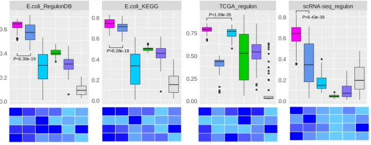
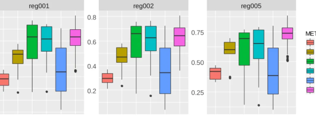
Figure 4. Overall performance comparison between QUBIC2 and five popular biclustering methods based on the agreement between identified biclusters and known modules. A. Distribution of F scores on each of the four datasets under multiple runs (n>40). Black line in the box denote median value, whiskers denote 10% and 90% percentiles, while the box denotes 25% and 75% percentiles; B. relative performance of six
algorithms in terms of F score under default parameters, variance of F scores under multiple sets of parameters, median value for the precision and median value for the recall, respectively (normalized over six algorithms). Note that the variance of F scores depends on the increment of
parameters, and therefore only indicative.
scRNA-seq_regulon reg002 reg005
0.25 0.50 0.75 0.0 0.2 0.4 0.6 0.8 0.0 0.2 0.4 0.6 0.8 METH H _ 0 .0 5 METH QUBIC2 QUBIC FABIA ISA Plaid Bimax
TCGA_regulon reg002 reg005
0.00 0.25 0.50 0.75 1.00 0.00 0.25 0.50 0.75 1.00 0.00 0.25 0.50 0.75 METH H _ 0 .0 5 METH QUBIC2 QUBIC FABIA ISA Plaid Bimax
E.coli_RegulonDB E.coli_KEGG ECO
0.0 0.2 0.4 0.6 0.0 0.2 0.4 0.6 0.8 0.0 0.2 0.4 0.6 METH H _ 0 .0 5 METH QUBIC2 QUBIC FABIA ISA Plaid Bimax simu_regulon 0.00 0.25 0.50 0.75 1.00 METH H _ 0 .0 1 METH QUBIC2 QUBIC FABIA ISA Plaid Bimax Default Variance Precision Recall R P V D
QUBIC2QUBIC FABIA ISA Plaid Bimax
METHS Va r1 0.00 0.25 0.50 0.75 1.00 value R P V D
QUBIC2QUBIC FABIA ISA Plaid Bimax
METHS Va r1 0.00 0.25 0.50 0.75 1.00 value R P V D
QUBIC2QUBIC FABIA ISA Plaid Bimax
METHS Va r1 0.00 0.25 0.50 0.75 1.00 value R P V D
QUBIC2QUBIC FABIA ISA Plaid Bimax
METHS Va r1 0.00 0.25 0.50 0.75 1.00 value R P V D
QUBIC2QUBIC FABIA ISA Plaid Bimax
METHS Va r1 0.00 0.25 0.50 0.75 1.00 value
scRNA-seq_regulon reg002 reg005
QUBIC2QUBICFABIA ISA PlaidBimax QUBIC2QUBICFABIA ISA PlaidBimax QUBIC2QUBICFABIA ISA PlaidBimax 0.25 0.50 0.75 0.0 0.2 0.4 0.6 0.8 0.0 0.2 0.4 0.6 0.8 METH H _ 0 .0 5 METH QUBIC2 QUBIC FABIA ISA Plaid Bimax R P V D
QUBIC2QUBIC FABIA ISA Plaid Bimax
METHS Va r1 0.00 0.25 0.50 0.75 1.00 value P=8.19e-8 P=6.30e-19 P=6.28e-19 P=1.09e-35 P=8.43e-39 A B
As showcased in Figure 4, QUBIC2 achieved the highest median F scores and the
highest F scores with the default parameter on all the four datasets, and its F scores were
significantly higher than the second-best algorithms in all the comparison circumstances (Wilcoxon test P-value <0.01). QUBIC2 performed well in both precision and recall,
indicating that the identified FGMs are relevant and diverse; and it had relatively small variance, while the performance of some algorithms on specific dataset was susceptible to parameter change (e.g., FABIA on E. coli). Regarding median F scores, QUBIC was the
second-best algorithm on simulated data, E. coli RNA-Seq data, and human scRNA-Seq
data, while FABIA was the second-best one for TCGA data. As regards the default settings, QUBIC ranked as the top ones on simulated data and E. coli data, and ISA and Plaid had
relative higher rank on TCGA data. ISA was generally very stable, and its variances were the smallest on three datasets. As for Bimax, although its recall was relatively low, it was characterized with high precision on the four datasets. It is noteworthy that QUBIC2 is the only program, among all the six biclustering algorithms, which did not encounter a dramatic performance drop on scRNA-Seq data compared to RNA-Seq data, suggesting the unique applicative power of QUBIC2 on FGMs detection from scRNA-Seq data.
Furthermore, the performance of all the biclustering algorithms on E. coli data was
better than on human data, with the possible reason that E. coli data has more completed
functional annotation and affects the evaluation of module significance. Therefore, for less annotated organisms, we need a statistical evaluation framework for all the identified biclusters.