Let Me Not Lie: Learning MultiNomial Logit
Brian Sifringera, Virginie Lurkinb, Alexandre Alahia
aVisual Intelligence for Transportation Laboratory (VITA), ´Ecole Polytechnique F´ed´erale de Lausanne (EPFL), Switzerland.
bDepartment of Industrial Engineering & Innovation Sciences, Eindhoven University of Technology, Eindhoven 5600MB, The Netherlands
Abstract
Discrete choice models generally assume that model specification is knowna priori. In prac-tice, determining the utility specification for a particular application remains a difficult task and model misspecification may lead to biased parameter estimates. In this paper, we pro-pose a new mathematical framework for estimating choice models in which the systematic part of the utility specification is divided into an interpretable part and a learning represen-tation part that aims at automatically discovering a good utility specification from available data. We show the effectiveness of our framework by augmenting the utility specification of the Multinomial Logit Model (MNL) with a new non-linear representation arising from a Neural Network (NN). This leads to a new choice model referred to as the Learning Multi-nomial Logit (L-MNL) model. Our experiments show that our L-MNL model outperformed the traditional MNL models and existing hybrid neural network models both in terms of predictive performance and accuracy in parameter estimation.
Keywords: Discrete choice models, Neural networks, Utility specification
1. Introduction
Discrete Choice Models (DCM) have emerged as a powerful theoretical framework for analyzing individual travel behavior. The goal of these models is to predict the choice among a given set of discrete alternatives (e.g., choice of walking as transportation mode rather than taking the car or the bus), while understanding the behavioral process that led to the specific choice. For many years, the Multinomial Logit Model (MNL) based on a linear utility specification has provided the foundation for the analysis of discrete choice. Despite its oversimplified assumptions regarding the actual decision-making, this model is still commonly used in practice because it enables a high level of interpretability.
Interpretability is critical for researchers and practitioners to get insights into the complex human decision-making process. For instance, linear specifications allow for straightforward derivation of the value-of-time (VOT), i.e., the marginal rate of substitution between time and cost, that constitutes a highly relevant measure in a wide range of public transport policy.
However, interpretability gain from using a MNL model with linear specification often leads to a sacrifice in the predictive power of the model. Indeed, MNL does not allow
to incorporate individual heterogeneity explicitly in the empirical investigation and the as-sumed linear statistical model cannot adequately capture the full underlying structure of the data. Several prior studies, within the discrete choice literature, have shown that incor-rectly assuming a linear utility specification can cause severe bias in parameter estimates and post-estimation indicators (e.g., Torres et al. (2011), Van Der Pol et al. (2014)).
More advanced utility specifications embedded into more complex models would allow for a better fit of the data and ultimately a better prediction. In this regard, utility specifications based on Box-Cox transformation, piecewise-linear, exponential, or non-parametric functions (e.g., Schindler et al. (2007), Kneib et al. (2007), Kim et al. (2016)), as well as advanced DCM models, such as the Mixed Logit Model (MLM) or the Latent Class Model (LCM), have been proposed in the literature (e.g., Shen (2009), Xiong and Mannering (2013), Vij et al. (2013), Kim et al. (2016)). However, the standard procedure for estimating the parameter values of these choice models is to assume that the model specification is known a priori, while in practice determining the utility specification for a particular application remains a difficult task.
Within the machine learning community, the field of representation learning is currently mastered by Neural Networks (NN). These models have become the go-to solutions, which have repeatedly demonstrated their superior prediction performance, including transporta-tion applicatransporta-tions (e.g., Omrani (2015), Hagenauer and Helbich (2017), Pekel and Soner Kara (2017), Nam et al. (2017), Pirra and Diana (2018)).
Unlike discrete choice models, these models require essentially no a priori beliefs about the nature of the true underlying relationships among variables. However, gaining in predic-tion accuracy often comes at the cost of losing interpretability, explaining why these models are often considered as a black-box by the discrete choice community.
In this work, we propose a new discrete choice modeling framework based on represen-tation learning to increase the predictive power of standard DCM without sacrificing their interpretability. Our proposal is to divide the systematic part of the utility specification into an interpretable part and a learning representation part that aims at automatically discov-ering a good utility specification from available data. This partially replaces manual utility specification and allows for a better prediction performance.
Using synthetic, semi-synthetic and real-world data, we demonstrate the effectiveness of our framework by augmenting the utility specification of the MNL model with a new non-linear representation arising from a neural network. It leads to a new choice model, referred to as the Learning Multinomial Logit (L-MNL). The source code is made publicly available to ease reproducibility and promote open science1.
The remainder of the paper is organized as follows: Section 2 is a non-exhaustive overview of the recent attempts to conduct multi-disciplinary research, combining machine learning and discrete choice modeling. Section 3, shows how the MNL model can be seen as a Convolutional Neural Network (CNN). Section 4 describes our proposed L-MNL model. Section 5, demonstrates evidence that our learning choice model outperforms both existing hybrid neural network and MNL models based on linear utility specifications. Our results show that the research community can benefit from a better integration of representation
learning techniques and discrete choice theory. In that sense, our research also contributes to bridge the gap between theory-driven and data-driven methods, and can encourage other researchers to exploit the power of such hybrid models.
2. Related work
Discrete choice and machine learning researchers have typically different perspectives and research priorities. The related work in each field is too broad to be covered here exhaustively and we therefore limit ourselves to the most relevant works at the intersection of the two communities.
More than 20 years ago, researchers were already interested in applying data-driven methods such as neural networks in different transportation applications (e.g., Faghri and Hua (1992), Dougherty (1995), Shmueli et al. (1996)). Over the years, different types of NN, as well as decision trees, have been compared to MNL models (Agrawal and Schorling (1996), Lee et al. (2018)), Nested Logit (NL) models (Mohammadian and Miller (2002), Hensher and Ton (2000)) and more generally to random utility models (Sayed and Razavi (2000), Cantarella and de Luca (2005), Paredes et al. (2017)) and statistical methods (West et al. (1997), Karlaftis and Vlahogianni (2011), Iranitalab and Khattak (2017), Golshani et al. (2018), Brathwaite et al. (2017)). However, the literature has mainly focused on comparing the models in terms of prediction power without discussing the issue of interpretability.
The machine learning community has also generated a tremendous amount of research aiming at predicting, with high accuracy, a variety of choices. Among the most recent works, Pekel and Soner Kara (2017) present a comprehensive review of publications related to the application of NN to predict travelers choice in public transportation. Hagenauer and Helbich (2017) compare seven machine learning methods to classify travel mode choice. The methods investigated are MNL and NN, but also Naive Bayes (NB) (Rish et al. (2001)), Gradient Boosting Machines (GBM) (Friedman (2001)), Bagging (BAG) (Breiman (1996)), Random Forests (RF) (Breiman (2001)), and Support Vector Machine (SVM) (Cortes and Vapnik (1995)). Pirra and Diana (2018) also propose to use SVM for travel mode choice while Lh´eritier et al. (2018) rely on RF and GBM to predict airline itinerary choice. Not surprisingly, the results exhibited in these papers show outstanding results in the ability of these models to fit to the data, but do not tackle the issue of their interpretability.
Some recent publications have attempted to go beyond the comparison of the two fields and proposed innovative behavioral studies based on data-driven methods. Two notable examples are the work of Wong et al. (2018), who use a restricted Boltzmann Machine (BM) (Ackley et al. (1985)) to represent latent behavior attributes, and the study of van Cranenburgh and Alwosheel (2019), who develop a novel NN based approach to investigate decision rule heterogeneity amongst travelers. However, these papers don’t have the ob-jective of finding an utility specification that allows high predictability while maintaining interpretability.
The closest studies relative to our work can be found in the brand choice literature. Bentz and Merunka (2000) introduce a hybrid model, afterwards called the NN-MNL model. Their model involves a two-stage approach that starts with the estimation of a NN model that aims at discovering non-linearity effects in the utility function. Then, if some non-linearities are
identified with the NN, the specification of the MNL model is modified to include new vari-ables, specially created to account for the discovered non-linear effects. On their database, the respecified MNL model, that includes the discovered non-linear effects, slightly outper-forms the basis MNL model. Their work, similar to ours in spirit, aims at achieving better predictive power together with a greater understanding of the influencing factors. However, their approach is sequential and their neural network is only used beforehand as a diagnostic and specification tool. Again, in the context of brand choice, Hruschka et al. (2002, 2004) and Hruschka (2007) investigate further the potential of neural network based choice mod-els. In Hruschka et al. (2002), the NN-MNL model is compared against homogeneous and heterogeneous versions of linear utility MNL models. Meanwhile in Hruschka et al. (2004), the comparison is done against two non-linear models, the generalized additive (GAM-MNL) model of Abe (1999) and a flexible functional form based on Taylor series approximations. The authors show that, by being capable of finding non-linear relationships from available data, the neural net based choice models with non-linear specifications outperform the other models in terms of prediction performance. But, by fully approximating the deterministic utility by means of a feedforward multilayer perceptron, the authors are unable to draw any conclusion regarding the significance of the factors and the postestimation analysis is limited to likelihood and choice elasticities. Finally, Hruschka (2007) proposes a Multinomial Probit (MNP) model with a neural net extension to model brand choice. Their model combines the heterogeneity across households with flexibility of the deterministic utility function, which is again achieved by means of a multilayer perceptron. Linear and non-linear deterministic utility specifications are considered but by specifying the same variables in linear and non-linear terms, the model loses its interpretability. The probit assumption also prevents the closed form of the choice probabilities and the model can only be estimated using a Markov Chain Monte Carlo simulation technique.
Our work significantly departs from these previous studies by proposing a flexible and general framework for the specification of the deterministic utility in any DCM model. More specifically, our approach combines, in a single joint optimization, the estimation of a stan-dard DCM model, based on a carefully thought utility specification, with a learning represen-tation model that aims at increasing the overall predictive performance. To our knowledge, this is the first formulation that benefits from the predictive power of representation learning techniques, while at the same time keeping some key parameters interpretable, which allows to derive insightful postestimation indicators. In Section 5 we show the effectiveness of our learning choice method by comparing its performance with benchmarking models, including the NN-MNL model of Hruschka et al. (2002, 2004).
3. Multinomial Logit and Convolutional Neural Network
Before introducing our learning choice model, we briefly show how the most popular discrete choice model, the Multinomial Logit (MNL), can be written as a weight sharing Neural Network by deriving equivalent mathematical expressions from both fields. Our method makes use of Convolutional Neural Networks (CNN) which are commonly used in signal-driven applications such as image classification (Krizhevsky et al. (2012)).
3.1. Multinomial Logit
Discrete choice modeling complies with the Random Utility Maximization (RUM) theory (McFadden (1974)) that postulates that an individual is a rational decision-maker that aims at maximizing the utility relative to her choice. Utility is a latent construct assumed to be partitioned into two components: a systematic (or deterministic) utility, Vin, and a random component,εin, that captures the uncertainty coming from the impossibility for the modeler to fully capture the choice context. Formally, the utility that individual n associates with alternative i from her choice set Cn is given as:
Uin=Vin+εin, (1)
For convenience, we consider the systematic part of the utility to be linear-in-parameter, as it is generally assumed:
Vin =
X
d
βd·xdin, (2)
whereβ are the preference parameters (or estimators) associated with the explanatory vari-ables (or the input features) x ∈ X that describe the observed attributes of the choice alternative (e.g., the price or travel time associated with the mode), and the individual’s socio-demographic characteristics (e.g., the individual’s level of income or age).
Under the standard MNL assumption thatεin
i.i.d.
∼ EV(0,1), the probability for individual
n to select choice alternative i is given by
Pn(i) =
eVin
P
j∈Cne
Vjn. (3)
The preference parametersβ are typically estimated by maximizing the log-likelihood func-tion given by:
L= N X n=1 X i∈Cn yinlog [Pn(i)], (4)
whereyin is the observed choice variable (or true label) and is equal to 1 if individualnchose the alternative i, and to 0 otherwise.
3.2. Multinomial Logit as Convolutional Neural Network
A neural network consists of a function mapping the input spacexto an output of interest
U through several intermediate representations commonly referred to as hidden layersh(j): U =h(L)(q(L−1)), (5)
with q(j)=h(j)(q(j−1)), ∀j = 1, ..., L, (6) where q(0) =xand Lis the last representation layer.
We make use of a Convolutional Neural Network (CNN) to retrieve the MNL formulation. A CNN has weights in the shape of a kernel that connect a layerh(j)to the next by applying
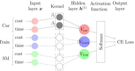
Car cost time Train cost time SM cost time βc βt Vcar Vtrain VSM CE Loss Softmax Kernel Input layerx Hidden layer h(1) Activation function Output layer
Figure 1: By aligning inputs by class and convolving with a kernel of equivalent shape and stride, we can retrieve linear utility specifications with a single CNN layer. By ending the network with a softmax activation layer and a cross-entropy (CE) loss, we retrieve the same formulation as for the MNL model.
a convolution2. Therefore, the value of a neuron i in the next layer (j + 1) can be written as: h(ij+1) =g( d X k=0 h((js)·i+k)βk(j)+α(ij)), (7) where {β1, ...βd} = β is a kernel of size (1×d), s the stride of the convolution, αi a bias term and g(·) an activation function.
The MNL formulation is retrieved by using a single layer (L= 1), setting the activation function to identity (g(x) = x) and the strides tod. Doing so, we get the utility functions Vn ={V1n, ...VIn} as defined in Equation (2).
Then, the probabilities can be obtained by using a softmax activation layer (Bishop (1995)) defined as: (σ(Vn))i = eVin P j∈Cne Vjn, (8)
which can be identified as Equation (3) for all probabilities. The output of the network goes through a loss function, in our case categorical cross-entropy (CE)(Shannon (1948)):
Hn(σ,yn) = −
X
i∈Cn
yinlog [σi(Vn)]. (9)
Minimizing (9) is equivalent to maximizing Equation (4) when summed over all individuals
n.
An illustrative example is given in Figure 1 with :
Uin=βc·x1i+βt·x2i+εin, ∀i∈ C, (10)
2Without loss of generality, we write the correlation formula. The operation is done without padding, effectively reducing the size from one layer to the next.
where x1 = cost stands for travel cost, and x2 = time for travel time. The choice set C
is assumed to be the same for all individuals and contains the following mode alternatives:
C ={Car, Train, Metro}. The kernel is made ofβ = (βt, βc), and a stride of d= 2 allows to recover each utility specification in the next layer fromcost and time of every alternative. 4. Learning Representation in Multinomial Logit
4.1. General Formulation
As previously mentioned, standard statistical procedure for estimating the parameter values of choice models is to assume that the correct utility specification is known a priori. Typically, the most common representation is inspired from linear regression and involves the observed attributes of the choice alternative and the individual’s socio-demographic characteristics. However, the influence of these explanatory variables on the utility of a choice alternative is unlikely to be known and to be precisely linear. The danger of an incorrect utility specification remains therefore highly present.
In this work, we propose a more flexible and data-driven approach that consists in ex-pressing the systematic part of the utility function into two subparts, as follows:
Vin=fi(Xn;β) +ri(Qn,w), (11) where
- f(Xn;β) is the assumed interpretable part of the utility specification. The function f is defined such that its unknown model parametersβ are an interpretable combination of the explanatory variables (or input features)Xn.
- r(Qn,w) is a representation that is learned from a set of explanatory variables (or input features)Qn, for which no a priori relationship is assumed.
Replacing the systematic utility component in Equation (1) by its new expression given by Equation (11), we obtain the following utility expression:
Un =f(Xn;β) +r(Qn;w) +εn. (12) Finally, in order to ensure that our learning model framework conserves the interpretabil-ity of behavioral choice models, we explicitly stipulate that the variables entering the inter-pretable part of the utility specification should be different than the input features of the representation learning. In other words, we impose that:
X ∩ Q=∅. (13)
Equation (13) constitutes a critical assumption which ensures that insightful postestima-tion indicators can be retrieved. The consequences of not defining disjoint sets of variables is further investigated in Section 5.
4.2. L-MNL Model Formulation
Given that Equation (12) is general, more specific assumptions regarding the distribution of the error term εin have to be made to derive operational learning choice models. Our learning choice model L-MNL follows the standard MNL assumptions described in Section 3.1. In particular, the interpretable part of the deterministic utility is assumed to be linear-in-parameter.
The likelihood of selecting the choice alternativeifor individualn, given the values of the model parameters (βand w) and the influencing factors (Xnand Qn), is therefore naturally expressed as: Pn(i) = efi(Xn;β)+ri(Qn;w) P j∈Cne fj(Xn;β)+rj(Qn;w). (14) Our L-MNL model uses a deep Neural Network (NN) as the learning method. More specifically, its representation term rin is the resulting function of a deep NN with L layers of H neurons and a single output per utility function:
rin = H
X
k=1
wik(L)g(q(nL−1)wk(L−1)+α(kL−1)) +α(iL), (15)
where g(·) is the rectifier linear units (ReLU) activation function and q(j)
n is recurrently defined by: h q(nj+1)i i = H X k=1 wik(j+1)g(qn(j)wk(j)+α(kj)) +α(ij+1), (16) with q(0)
n being the vector of input features Qn.
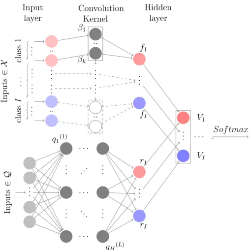
The architecture of our L-MNL hybrid model is shown in Figure 2, where we see both the linear component, written as a CNN (see Section. 3), and the representation term, obtained through a deep NN.
5. Experiments
Our experiments demonstrate how our L-MNL model is able to increase thepredictability
of the MNL model while keeping itsinterpretability. The former,predictibilty, can be directly quantified in terms of likelihood. The latter interpretability, however, is more challenging to assess. To do so, we define interpretability as the ability of the model to recover the true parameters’ values of the variables that enter the interpretable part of the utility function. We run two types of experiments: (i) using synthetic and semi-synthetic data for which the true estimates of interpretable parameters are known and (ii) using real-world data for which true estimates are not known. For each experiment, we compare our L-MNL model performance with benchmarking models from previous works.
.. . .. . class 1 .. . .. . ... .. . class I .. . Inputs ∈ X β1 βk .. . .. . .. .. .. .. f1 .. . fI Convolution Kernel Input layer Hidden layer V1 .. . . . . VI Sof tmax .. . Inputs ∈ Q q1(1) qH(L) .. . .. . .. . .. . . . . . . . . . . . .. . .. r1 .. . rI
Figure 2: L-MNL model architecture. On the top, we have theIclass generalization of a linear-in-parameter MNL model, as depicted in Figure 1. At the bottom, we have a deep neural network (i.e., multilayer and fully connected) that enables us to obtain the representation learning termri. The terms from each part are added together defining the new systematic function of Equation (11).
5.1. Benchmarking models
Our learning choice framework is both general and flexible. On one hand, theoretically, any architecture can be chosen for the neural network. On the other hand, the feature selec-tion process is driven by the modeler, knowing which variables have to be in the interpretable utility specification to get the needed insightful postestimation indicators. Interestingly, existing hybrid models from the literature can be retrieved with appropriate assumptions regarding the following decisions:
1. Which explanatory variables are kept in the interpretable part of the utility specifica-tion (i.e., the subset variables X)?
2. Which explanatory variables are given as input features to the neural network (i.e., the subset variables Q)?
3. Which architecture is chosen for the neural network (i.e., the r function in Equation (12))?
Thus, the neural network proposed by Bentz and Merunka (2000), afterwards extended by Hruschka et al. (2002, 2004), is obtained by assuming that there is no variable in the linear part of the utility specification and that all variables are therefore given as input features to the neural network. Their neural network architecture is given by:
rin = H
X
k=1
βk(2)g(βk(1)qin+αk), (17) where g(·) is a sigmoid activation function.
Equation (17) applies the same neural network layer on each alternative i separately, much like our CNN depicted in Figure 1, but with dense connections between the input layer and the kernel. Although their model shows very good predictive performance, it remains a ‘black box’ since no variable enters the interpretable part of the utility specification (X =∅). In our experiments, we want to compare our L-MNL model in terms of both prediction performance and level of accuracy obtained for the parameter estimates. Therefore, we also use as a benchmark the NN-MNL model proposed by Hruschka et al. (2002, 2004) but with an utility specification inspired by Hruschka (2007). More specifically, we combine a linear-in-parameter utility specification with a non-linear learning representation that is obtained using the same neural network. All variables are used both as explanatory variables in the interpretable utility specification, and as input features to the neural network.
Finally, it is worth mentioning that the standard linear-in-parameter MNL model can also be expressed as a L-MNL model by assuming that there is no variable given as input features to the neural network and that all carefully chosen explanatory variables enter in the interpretable part of the utility specification. Essentially, we compare the following models:
• Logit(X): The standard MNL model with linear-in-parameter specification, and no learning component. The variables x ∈ X enter the linear utility specification and
Q=∅.
• Hruschka(n,Q): The NN-MNL model proposed by Hruschka et al. (2004) with n
neurons in the hidden layer (H = n). The variables x ∈ Q are the input features of the neural network. There is no variable entering the linear utility specification. The function r(Q) is defined by Equation (17).
• Hruschka(n,X =Q): A modified version of the NN-MNL model proposed by Hruschka et al. (2004). The variables x∈ X(= Q) enter both the linear utility specification and the neural network. The function r(Q) is defined by Equation (17) with n neurons in the hidden layer (H =n).
• L-MNL(n,X,Q): Our learning logit model withnneurons in the hidden layer (H =n). Part of the variables x ∈ X enter the linear utility specification and the remaining variables x ∈ Q (X ∩ Q =∅) are given as input features to the neural network. The function r(Q) is defined by Equation (15).
5.2. Synthetic data
Using synthetic data, we show how our L-MNL model performs better than the stan-dard linear-in-parameter MNL model in terms of both prediction performance and estimates
accuracy. We start by describing how we generated the synthetic data. Then, we perform Monte Carlo experiments to compare all benchmarking models on parameters estimation. We proceed with additional experiments to study the particular effects of correlated or miss-ing variables. Finally, an arbitrary example is introduced to better analyze the impact of the NN architecture, and also the effects of sequential versus joint optimization strategies.
5.2.1. Data generation
Synthetic data provide a controlled environment for analyzing our L-MNL model. To generate our synthetic data, we consider a simple binary choice model where an individual
n has to choose to take a specific action or not (e.g., choosing to use public transportation to go to work as opposed to not using public transportation). We consider that the utility obtained for taking the action is given by
Un=Vn+εn, (18) with Vn=β1·x1+β2·x2 | {z } known relation +β3·x3x4 +β4·x3x5 | {z } unknown interactions , (19)
where we consider the non-linear interactions among variables to represent unknown and undiscovered causalities.
In order to construct our synthetic observations, we need to generate individual values for the explanatory variables (or features) x, as well as for the synthetic choices (or labels)
y, i.e., the individual’s decisions to take (yn= 1) or not (yn = 0) the action. For the explanatory variables, we assume that
xk∼ N(0,1), ∀k = 1, ...5. (20) Under the classical logit assumption that εn
i.i.d.
∼ EV(0,1) and given fixed values of parameter estimates βin the utility specification, the choice probabilities Pn(x) are known, and the synthetic choice yn can then be seen as a Bernoulli random variable that takes the value 1 with probabilityPn(x) and 0 with probability 1−Pn(x). Formally, we assume that
yn ∼Bern (Pn(x)), ∀n= 1, ...N. (21)
Using synthetic data allows us to compare our L-MNL model with standard choice models, not only in terms of prediction performance, but also in accuracy in parameter estimation since we know the true value of parameter estimates β, i.e., the true linear and non-linear dependencies between the variables.
5.2.2. Monte Carlo experiment
We rely on Monte Carlo simulations to investigate how well each model performs in both prediction and parameter estimation of Equation (19). To do so, we assume that the β
coefficients follow an uniform distribution:
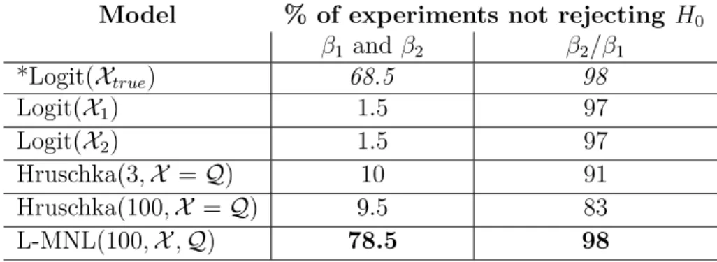
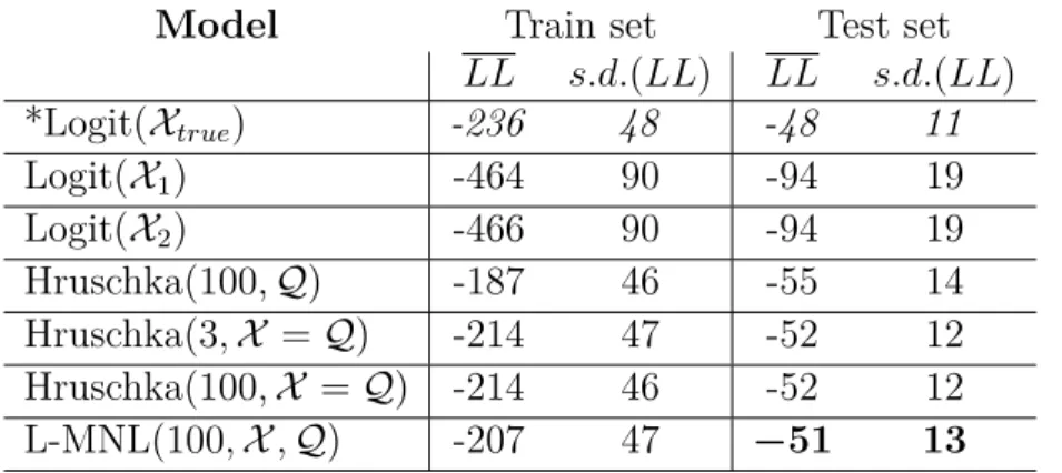
Table 1: Monte Carlo average log-likelihood ( ¯LL) and standard deviation (s.d.(LL)) for the different models. Based on the test set value, we conclude that our L-MNL learns the best general representation. A MNL model with true utility specification is given as a reference.
Model Train set Test set
LL s.d.(LL) LL s.d.(LL) *Logit(Xtrue) -236 48 -48 11 Logit(X1) -464 90 -94 19 Logit(X2) -466 90 -94 19 Hruschka(100,Q) -187 46 -55 14 Hruschka(3,X =Q) -214 47 -52 12 Hruschka(100,X =Q) -214 46 -52 12 L-MNL(100,X,Q) -207 47 −51 13
and we randomly sample 100 times from that distribution. For each utility specification thus obtained, we generate 1,000 synthetic individual observations for the training set, and 200 more for the testing set.
Our learning choice model is defined as
• L-MNL(100,X,Q), withX ={x1, x2}, and Q={x3, x4, x5},
and is compared with the following five benchmarking models and one reference model*3:
• Logit(X1), withX1 ={x1, x2, x3, x4, x5},
• Logit(X2), withX2 ={x1, x2},
• Hruschka(100,Q), with Q={x1, x2, x3, x4, x5},
• Hruschka(3,X =Q), withX =Q={x1, x2, x3, x4, x5},
• Hruschka(100,X =Q), with X =Q={x1, x2, x3, x4, x5},
• *Logit(Xtrue), with Xtrue={x1, x2, x3x4, x3x5}.
The log-likelihood results from Monte Carlo experiments can be seen in Table 1. As expected, the best models in terms of predictive performance are the neural net based choice models. Among them, in despite of a slight overfitting on the train set, our L-MNL gives the best general representation of the data, achieving the best predictive performance in the test set (with a LL of -51 compared to -94 for the standard MNL models).
3The reference model is considered differently than the benchmarks as it breaks the assumption that the modeler does not know the ground truth.
Table 2: Monte Carlo relative errors for the different models in [%] withethe average relative error,s.d.its standard deviation andβ1,β2 are from Equation (19).
Model eβ1 s.d.(eβ1) eβ2 s.d.(eβ2) eβ2/β1 s.d.(eβ2/β1) *Logit(Xtrue) 11.7 ± 8.3 12.6 ± 7.8 6.15 ± 7.1 Logit(X1) 50.4 ± 11.4 51.6 ± 11.6 9.9 ± 8.8 Logit(X2) 50.1 ± 11.1 52.0 ± 11.3 10.0 ± 8.7 Hruschka(3,X =Q) 37.4 ± 13.7 39.1 ± 13.0 13.2 ± 11.5 Hruschka(100,X =Q) 36.7 ± 13.9 38.6 ± 15.7 16.6 ± 16.8 L-MNL(100,X,Q) 9.2 ± 8.2 8.5 ± 8.5 6.7 ± 8.0
In order to evaluate the models in terms of accuracy in interpretable parameter estima-tion, we define the relative errors eβ and eβi/βj as
eβ = β−βb β , (23) eβi/βj = eβi−eβj 1−eβj . (24)
The relative error results4 from Monte Carlo experiments can be seen in Table 2. We see that our L-MNL greatly outperforms every model in the ability to recover the true parameter values with a relative error smaller than 10%. It is worth noting that for the ratios of parameters, the MNL models perform second best, although they have high relative errors at parameters level. This phenomenon has been investigated in a few papers (e.g., Lee (1982), Cramer (2007)) where it has been shown that even when utility is misspecified, the MNL model is still able to retrieve good ratios between estimates. The hybrid models with X = Q on the other hand generate high errors in parameter estimates. It seems to indicate that the NN component is also partially learning linear dependencies of x1 or x2,
and prevents the linear functionf to reach a minimum as good as our L-MNL. Interestingly, we also see that the small overfit on the variables in Q = {x3, x4, x5} of the training set
allows the L-MNL to better retrieve the coefficients associated with X when compared to the reference model. In other words, some of the complexities from the random generation process are learned by the NN, leading to a better fitting for the interpretable terms.
Finally we conduct hypothesis testing to determine whether the estimated parameters are statistically different from the true ones. Formally, we consider the following null and alternative hypotheses: H0 :βb=β, and H1 :βb6=β.
The results are shown in Table 3. We see that the coefficients alone are almost always statistically different for every model except L-MNL. The NN component of our model fixes the estimators by learning only on the data that are independent from the linear component. The ratio of parameters on the other hand is well retrieved with both MNL and L-MNL models. Concerning the hybrid Hruschka benchmarking models, we see that their
4Note that the Hruschka(100,Q) benchmarking model does not appear in Table 2 since no variable enters the linear utility specification.
Table 3: Monte Carlo hypothesis testing for the different models, for β1 and β2 taken separately and for their ratio. Parametersβ1,β2 are from Equation (19).
Model % of experiments not rejecting H0 β1 and β2 β2/β1 *Logit(Xtrue) 68.5 98 Logit(X1) 1.5 97 Logit(X2) 1.5 97 Hruschka(3,X =Q) 10 91 Hruschka(100,X =Q) 9.5 83 L-MNL(100,X,Q) 78.5 98
NN component compromises the ratios between parameters. Indeed, the higher number of neurons in the network, the more the learning overlap between the representation term and the linear term creates errors on the parameter ratios. Finally, we observe once again a slight overfit for our model when comparing to the reference. Indeed, we have a higher expectation in retrieving the true values of the β1 and β2.
To better illustrate the origin of ratio discrepancy whenX ∩ Q 6=∅in hybrid models, we show in the next subsection that we retrieve the same biasing effect on our L-MNL when we make use of perfectly correlated data between both sets.
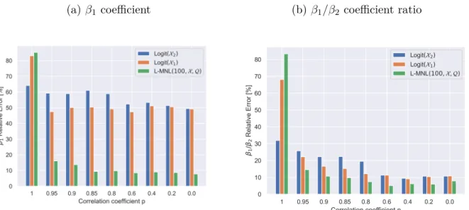
5.2.3. Impact of correlated variables
Experimental results from Section 5.2.2 suggest that having identical variables (or fea-tures) in both sets lead to poor parameter estimates because of the neural network’s better ability to discover the true relationship between variables.
Although our L-MNL requests the variables in the two sets to be different, strong cor-relation between the variables can remain an issue. To investigate the impact of correlated variables, we replace the original explanatory variable x3 with a new explanatory variable x03 that is defined to be correlated to x1. Formally, we define x03 as
x03 =p·x1+ q
1−p2·x
3, (25)
where p∈(0,1) is the correlation coefficient. Our learning choice model is defined as
• L-MNL(100,X,Q), withX ={x1, x2}, and Q={x03, x4, x5},
and is compared with the following two benchmarking models:
• Logit(X1), withX1 ={x1, x2, x03, x4, x5},
• Logit(X2), withX2 ={x1, x2}.
The Monte Carlo mean relative errors for different levels of correlation are shown on Figure 3. We see that for the not perfectly correlated cases (p ≤ 0.95), our L-MNL has
(a)β1 coefficient (b)β1/β2 coefficient ratio
Figure 3: Impact of correlated variables on parameter estimates, wherex1∈ X is correlated tox03∈ Q(see Eq.25). We see the models with correlated inputs only suffer in this case for very high correlations (>0.95)
low relative errors in parameter estimates compared to the MNL models. However when the variables are perfectly correlated, the relative error becomes larger. This again shows the NN’s capability of learning linear relations, which interferes with the linear specifica-tion. This is important as it suggests that in order to get insightful results, the modeler has to carefully check that the variables that enter as input features in the neural network are not the same or not too highly correlated with the variables in the linear utility specification.
5.2.4. Impact of unseen variables
We take advantage of synthetic data to better analyze the impact of unseen variables on parameter estimates. To do so, we assume that we know the following true utility specifica-tion:
Vn0 =Vn+β5·x6·x7, (26)
where Vn is given by Equation (19).
We assume that variables x6, x7 ∼ N(0,1) are unobserved by the modeler, i.e., that x6, x7 ∈/ (X ∪ Q). We also assume that β5 follows the distribution of Equation (22) and we
randomly sample 100 times all β parameters. For each utility specification thus obtained, we generate 1,000 synthetic observations for the training set and 200 more for the testing set.
Our learning choice model is defined as
• L-MNL(100,X,Q), withX ={x1, x2} and Q={x3, x4, x5},
and is compared with the following benchmarking model:
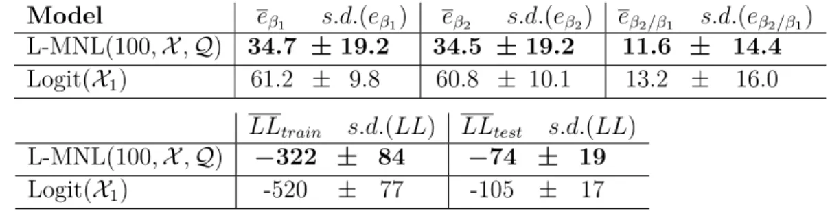
Table 4: Impact of unseen variables on parameter estimates and log-likelihood. e is the average relative error,s.d.its standard deviation andβ1, β2 are from Equation (19).
Model eβ1 s.d.(eβ1) eβ2 s.d.(eβ2) eβ2/β1 s.d.(eβ2/β1) L-MNL(100,X,Q) 34.7 ± 19.2 34.5 ± 19.2 11.6 ± 14.4 Logit(X1) 61.2 ± 9.8 60.8 ± 10.1 13.2 ± 16.0 LLtrain s.d.(LL) LLtest s.d.(LL) L-MNL(100,X,Q) −322 ± 84 −74 ± 19 Logit(X1) -520 ± 77 -105 ± 17
The Monte Carlo mean relative errors for the two models are shown in Table 4.
We see that, compared to the results depicted in Table 2 where all variables in the true
utility specification had been included in the models, the unseen variables lead, for both models, to a decrease in the fit and an increase in relative errors in parameter estimates. Nevertheless, our L-MNL still continues to perform better than the MNL model since it achieves a better fit (LL of -74 compared to -105) with smaller relative errors in parameter estimates (11.6 compared to 13.2).
5.2.5. Illustrative example
To investigate the best L-MNL architecture and optimization strategy, we make use of the following nonlineartrue utility specification:
Vn00 = 2·x1+ 3·x2+ 0.5·x3·x4+ 1·x3·x5, (27)
and we generate a synthetic dataset of 10,000 individual observations for the train set and 2,000 for the test set.
Our learning choice model is defined as
• L-MNL(100,X,Q), withX ={x1, x2} and Q={x3, x4, x5},
and is compared with the following standard linear-in-parameter logit model:
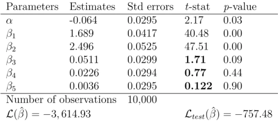
• Logit(X1), withX1 ={1, x1, x2, x3, x4, x5}.
The results of the MNL model are depicted in Table 5. We see that all nonlinear in-teractions in the true utility specification Vn0 lead to insignificant parameter estimates at significance level α= 0.05 (p-value>0.05). Linear-in-parameter coefficient estimates of our L-MNL model are depicted in Table 6. We see that all estimates are significant (p-value >
0.05), and that the neural network highly contributes to improve the predictive performance of the model (the final likelihood increases from -3,616 to -3,090).
Furthermore, for both models, we want to test if the estimated parameters βb1 and βb2
are statistically different from their true values of β1 = 2 and β2 = 3. The results of
the hypothesis tests are depicted in Table 7. We see that thanks to the neural network component, our learning choice model is able to retrieve parameter estimates that are not statistically different from their true values, while the estimates from the linear-in-parameter model are statistically different from the true ones. This is important as it confirms that utility misspecification leads to incorrect parameter estimates and that L-MNL has the potential to recover the true relationship among the variables.
Table 5: Logit(X1) withX1={x1, x2, x3, x4, x5}. Ground truth: β1= 2 and β2= 3.
Parameters Estimates Std errors t-stat p-value
α -0.064 0.0295 2.17 0.03 β1 1.689 0.0417 40.48 0.00 β2 2.496 0.0525 47.51 0.00 β3 0.0511 0.0299 1.71 0.09 β4 0.0226 0.0294 0.77 0.44 β5 0.0036 0.0295 0.122 0.90 Number of observations 10,000 L( ˆβ) =−3,614.93 Ltest( ˆβ) = −757.48
Table 6: L-MNL(100,X,Q) withX ={x1, x2} andQ={x3, x4, x5}. Ground truth: β1= 2 andβ2= 3.
Parameters Estimates Std errors t-stat p-value
β1 1.999 0.0452 44.24 0.00
β2 2.929 0.0567 51.61 0.00
Number of observations 10,000
L( ˆβ) =−3,090.09 Ltest( ˆβ) = −659.36
5.2.6. Choice of neural network architecture
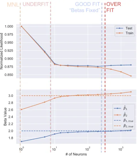
Choosing the structure of a NN requires to have enough capacity to capture the under-lying pattern of the data without overfitting. In the following, we gradually increase the size of the NN component in L-MNL, spanning from an underfit of the non-linear truth of Equation (27) to an overfit of the generated data. To illustrate these effects, we study the values of β1 and β2, as well as likelihoods of both train and test sets.
The results are depicted in Figure 4, where we take L-MNL(n,X,Q) with a single layer L=1, and scan from n = 0 neurons in the hidden layer to n = 5000. We see that from n = 0 neurons (≡MNL) to about n= 10, the NN has not yet captured all the non-linearities of the original utility specification. This can be seen by the higher values in likelihood and how the parameter estimates have not yet reached their true minimum. From n= 10 ton= 200, the model reaches stable values where the linear terms are equivalent to their ground truth. The NN component has successfully learned the non-linearities of the data. When we continue to increase the number of neurons, we see the effects of overfit, namely a drop in train likelihood and an increase in test likelihood. We finally observe that the values ofβ1 andβ2 also suffer
from the overfit, as the L-MNL is no longer a general representation of the data, but has become specific to the training set.
5.2.7. Optimization Strategy
As depicted in Figure 2, our L-MNL architecture contains two parts: the top of the figure represents the linear component in the utility specification, while the bottom depicts the learning component. The number of parameters to be estimated in each part can vary
Table 7: Results of hypothesis testing on synthetic data.
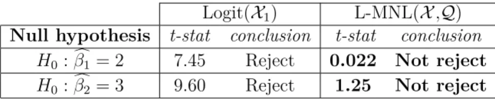
Logit(X1) L-MNL(X,Q) Null hypothesis t-stat conclusion t-stat conclusion
H0 :βc1 = 2 7.45 Reject 0.022 Not reject H0 :βc2 = 3 9.60 Reject 1.25 Not reject
significantly. While a limited number of parameters are generally included in linear specifica-tion, a neural network can easily contain thousands of parameters. Given this architecture, one could be tempted to estimate the model sequentially. To show the importance of jointly estimating the parameters, we consider the three following strategies for estimating our L-MNL(100,X,Q):
1) First optimizing the linear specification (i.e., theβ parameters) and then learning the representation term after fixing the previously found linear-in-parameter estimates. 2) First optimizing the representation term (i.e., the w weights) and then learning the
linear specification after fixing the previously estimated weights. 3) Optimizing jointly both components.
Results are shown in Table 8. We see that the joint optimization allows for the best minima in both likelihood and parameter estimation. Starting with the linear specification gives the same parameters as for MNL (Table 5), but with a better likelihood. The second strategy, on the other hand, reaches a sub-optimal minima when learning the representation. It is only with joint optimization that all important explanatory variables are expressed. The two components complete each other to achieve the best prediction performance with the correct parameter values.
Table 8: Values of parameter estimates and likelihoods based on optimization strategy forβ1= 2 andβ2= 3. Best results are obtained with joint optimization.
Strategy βˆ1 βˆ2 LL
(1) βˆ then w 1.62 2.48 -3100 (2) w then βˆ 1.72 2.65 -3197 (3) βˆ and w 1.98 3.02 -3040
5.3. Semi-Synthetic Data
In this section, we challenge our L-MNL model by analyzing its effectiveness outside of fully synthetic data and in the presence of strong non-linearities. We first start with experiments on semi-synthetic data before moving to real data in the next Section. To
MNL
UNDERFIT OVER FIT GOOD FIT “Betas Fixed”Figure 4: Likelihood and values of parameter estimates for an increasing number of neurons in the hidden layer. Best results are obtained withn∈[10,200]
generate our semi-synthetic data, we follow the same procedure as before, but instead of using normally distributed explanatory variables, we randomly select them from a real world dataset, the Swissmetro dataset (Bierlaire et al. (2001)).
The SwissMetro dataset consists of survey data collected in Switzerland, during March 1998. The respondents provided information in order to analyze the impact of a new inno-vative transportation mode, represented by the Swissmetro, a revolutionary mag-lev under-ground system. Each individual reported the chosen transportation mode choice for various trips including the car, the train or the Swissmetro.
We define the following utility specifications:
VT rain= lT rain + 1·DEST3·AGE −1·AGE0.5·ORIGIN
VSM = lSM + 1·DEST·AGE + 3·IN COM E5·P U RP OSE2
Table 9: Variables in the Swissmetro dataset used for experiments on semi-synthetic data
Variable Description
TT Door-to-door travel time in [minutes]. TC Travel cost in CHF.
Purpose Trip purpose (business, leisure, etc.) Income The traveler’s income per year.
Origin The canton in which the travel begins. Dest The canton in which the travel ends. Age The traveler’s age.
with
li =−1·T Ti−2·T Ci ∀i∈ C, (29) The coefficients are chosen in order to have a balanced dataset, and the interacting variables are the categorical features of Swissmetro data (Bierlaire et al. (2001)) and are described in Table 9. Note that we have chosen to use power series to complexify the non-linear terms.
The models under study are:
• Logit(Xa) with linear-in parameters utility specification based on the following features: – XT rain,a ={1,T TT rain, T CT rain, AGE, DEST, ORIGIN}
– XSM,a ={1,T TSM, T CSM, AGE, DEST, IN COM E, P U RP OSE} – XCar,a ={1,T TCar, T CCar, AGE, ORIGIN, IN COM E}
• Logit(Xb) with only travel time and cost for each utility, i.e.: – Xib ={1, T Ti, T Ci} for all i∈ C.
• L-MNL(X, Q) with – Xi ={T Ti, T Ci},
– Q={AGE, DEST, ORIGIN, IN COM E, P U RP OSE}
The results can be seen in Table 10. We see that standard MNL models are unable to retrieve the correct parameter estimates for utility specifications with important non-linearities. Both MNL models exhibit large relative errors (about 40% for the Logit(Xb) and at least 25% for the Logit(Xa)). The relative errors are also large for the ratio of parameters, which would lead to wrong postestimation indicator, the VOT in this case. Unlike the Logit models, our L-MNL model recovers the true estimates in both parameters and ratio, while achieving a much better fit. We therefore conclude that the representation term was able to learn the complex non-linearities and that ignoring these non-linearities lead to models that greatly suffer from underfit.
Table 10: Values of parameter estimates and likelihoods for different models based on Equation (28). Ground truth isβ1=−1 andβ2=−2. Only L-MNL is able to estimate correctly the parameters.
Models βˆ1 βˆ2 βˆ2/βˆ1 LLtrain LLtest
Logit(Xa) -0.65 -1.63 2.50 -5412 -1354
Logit(Xb) -0.25 -0.70 2.81 -7722 -1925
L-MNL(X,Q) −1.01 −1.99 1.96 −2516 −809
Table 11: Swissmetro benchmark utility function, from Bierlaire et al. (2001)
Alternative
Variables Car Train Swissmetro
ASC Constant Car-Const SM-Const
TT Travel Time B-Time B-Time B-Time
Cost Travel Cost B-Cost B-Cost B-Cost
Freq Frequency B-Freq B-Freq
GA Annual Pass B-GA B-GA
Age Age in classes B-Age
Luggage Pieces of luggage B-Luggage
Seats Airline seating B-Seats
5.4. A real case study: the SwissMetro dataset
While the experiments on synthetic and semi-synthetic datasets have demonstrated the benefits of our learning choice model, we finally want to study its performance on real-world data containing âĂIJtrueâĂİ choices made by individuals. For these experiments, we con-tinue to use the openly available dataset SwissMetro but with the real choices (Bierlaire et al. (2001)). The original dataset contains 10,728 observations. We removed observations for which the information regarding the chosen alternative was missing (9 observations) and for convenience we also decided to discard the observations for which the three alternatives car, train, and swissmetro were not all available (1,683 observations). Our dataset con-tains therefore 9,036 observations. We split this initial dataset into a training set of 7,234 observations and a test set of 1,802 observations.
5.4.1. Models Comparison
Since the true values of parameter estimates are unknown, we compare the values ob-tained with our L-MNL to the ones obob-tained using the MNL model described in Bierlaire et al. (2001), whose linear-in-parameter utility specification is described in Table 11. The results of parameter optimization for this MNL model are shown in Table 13a5.
5It is worth noting that the values of estimates that we obtain slightly differ from the ones depicted in the original paper. This is normal since the original Swissmetro dataset is different from the training dataset that we used.
Table 12: Unused variables in the Swissmetro dataset
Variable Description
Purpose: Integer variable indicating the trip purpose (business, leisure, etc. ) First : Binary variable indicating if first class (=1) or not (=0)
Ticket: Integer variable indicating the ticket type (one-way, half-day, etc.) Who: Integer variable indicating who is paying the ticket (self, employer, etc.) Male: Binary variable indicating the traveler’s gender (0 = female, 1 = male) Income: Integer variable indicating the traveler’s income per year.
Origin: Integer variable indicating the canton in which the travel begins. Dest: Integer variable indicating the canton in which the travel ends.
We next estimate the learning choice model L-MNL(100,X1,Q1), where X1 contains the
same variables as the ones included in the utility specification of Bierlaire et al. (2001), and
Q1 contains all the unused variables in the dataset. These variables are described in Table
12. The results of this model are depicted in Table 13b.
We see that adding the neural network learning component in the utility specification significantly increases the log-likelihood, suggesting that these variables contain information that helps to explain travelers’ choice. However, we also see that several estimates are not statistically different from zero (p-value > 0.05). We have seen in Section 5.2.3 that corre-lation between variables can lead to biased parameter estimates. However, the correcorre-lation among the variables has been investigated and does not seem to be the issue here (see Table A.15 in Appendix for the correlation among variables). Moreover, the Hruschka(100,X1 =Q)
model (see Table 13c) has one-to-one correlation among variables in both sets and does not loose significance in its parameters. Therefore, the coefficients in L-MNL have most likely lost their significance due to the neural network’s ability to better learn causality from the data. The significance of the same parameters in the initial MNL model can originate from a bias due the model’s underfit. In addition, with many explanatory variables being omitted in the initial MNL model, it is worth noting that the model is more likely to be subject to endogeneity, i.e.— correlation among the dependent variables and the error term. Endo-geneity is a well-known cause of biais in parameter estimates and can therefore also cause biais in the parameter estimates of the initial MNL model.
Finally, we noticed that two key postestimation indicators were reported in Bierlaire et al. (2001): the Value of Time (VOT) and Value of Frequency (VOF). These ratios are important indicators to get insights into the complex human decision-making process and are highly relevant measures for public transport policy makers. In consequence, we decided to estimate the learning choice model L-MNL(100,X2,Q2), whereX2 contains only the variables needed
to compute the VOT and VOF, i.e., the variables time, cost, and f requency. All other variables constitute the set Q2 and are therefore given to the neural network. The results
performed by this hybrid model with H = 100 can be seen in Table 13d.
We observe that all parameter estimates are significant, while the log-likelihood has greatly increased compared to the standard MNL model. In other words, the representation term was able to get information from the previsouly non-significant variables in the linear specification.
Table 13: Comparison of parameters estimates for different models with utility specification of Bierlaire et al. (2001)
(a)Parameter estimates from MNL model
Parameters Estimates Std errors t-stat p-value
ASCCar 1.08 0.162 6.67 0.00 ASCSM 1.05 0.153 6.84 0.00 βage 0.146 0.436 3.35 0.00 βcost -0.695 0.0423 -16.42 0.00 βf req -0.733 0.1132 -6.47 0.00 βGA 1.54 0.167 9.24 0.00 βluggage -0.114 0.0488 -2.338 0.02 βseats 0.432 0.115 3.76 0.00 βtime -1.34 0.051 -26.18 0.00 Number of observations 7,234 L( ˆβ) =−5764 Ltest( ˆβ) =−1433
(b) Parameter estimates from L-MNL(100,X1,Q1) model
Parameters Estimates Std errors t-stat p-value
ASCCar 0.106 0.174 0.61 0.54 ASCSM 0.454 0.163 2.80 0.01 βage 0.390 0.045 8.63 0.00 βcost -1.378 0.048 -28.45 0.00 βf req -0.860 0.127 -6.77 0.00 βGA 0.214 0.194 1.10 0.27 βluggage 0.116 0.0529 2.19 0.03 βseats 0.104 0.109 0.95 0.34 βtime -1.563 0.056 -27.97 0.00 Number of observations 7,234 L( ˆβ) =−4511 Ltest( ˆβ) =−1181
(c) Parameter estimates from Hruschka(100,X1 =
Q) model
Parameters Estimates Std errors t-stat p-value
ASCCar 0.365 0.165 3.61 0.00 ASCSM 0.549 0.162 2.22 0.03 βage 0.087 0.0423 2.07 0.04 βcost -0.897 0.046 -19.46 0.00 βf req -0.639 0.123 -5.20 0.00 βGA 1.40 0.172 8.15 0.10 βluggage 0.186 0.0523 3.52 0.00 βseats 0.233 0.102 2.29 0.02 βtime -1.146 0.049 -23.32 0.00 Number of observations 7,234 L( ˆβ) =−4964 Ltest( ˆβ) =−1257
(d) Parameter estimates from L-MNL(100,X2,Q2) model with new linear specification
Parameters Estimates Std errors t-stat p-value
βcost -1.587 0.0500 -31.75 0.00
βf req -0.869 0.0757 -11.48 0.00
βtime -1.758 0.0416 -42.28 0.00
Number of observations 7,234
L( ˆβ) =−3968 Ltest( ˆβ) =−1107
We show a comparison of VOT and VOF for the different models in Table 14. Based on our multiple experiments on synthetic and semi-syntehtic data, we believe that our L-MNL provide better estimates, and therefore more realistic VOT and VOF. The important difference in log-likelihood values between the L-MNL and the Logit(X1) suggests that the
MNL model suffers from underfitting that leads to important ratio discrepancy, as shown in Section 5.3. The linear specification of the MNL model does not allow to capture the Swissmetro’s non-linear dependencies among variables.
In support of these conclusions, we incrementally increase the size of the NN component. We observe in Figure 5 the parameter values with respect to the number of neurons in our neural network. As for the illustrative example of the Section 5.2.5, we see that stable ratios for VOT and VOF are obtained for a neural network having from 10 to 200 neurons. We see the MNL ratios for n=0 neuron, highlighting the underfit of the MNL model. An overfit effect is observed starting from 500 neurons, where the test likelihood no longer improves.
Table 14: Parameter ratio comparison
Model Logit(X1) Hruschka(100,X1 =Q1) L-MNL(X1) L-MNL(X2)
Value of Time 0.52 0.78 0.88 0.90
Value of Frequency 0.95 1.40 1.60 1.82
Train Log-Likelihood -5764 -4964 -4511 -3968
Test Log-Likelihood -1433 -1257 -1181 -1107
MNL
Stable Estimators
OVERFIT
Figure 5: Scan of Likelihood and Beta values over number of neuronsnin the densely connected layer for L-MNL(100,X2,Q2). For n∈ [10,200] we have VOT≈1 and VOF≈1.9. Overn = 200, we have signs of overfit.
(a) (b)
Figure 6: Change in total mode shares against percentage change in L-MNL features belonging toQ2. These general trends appear by fixing all other values as constant.
5.4.2. Feature impact and sensitivity analysis
As previsously done by Bentz and Merunka (2000), we finish our experiments by inves-tigating what the neural network component has learned through the study of a sensitivity analysis. To do so, we vary the value of a feature in Q while keeping the others variables constant, and we analyze its impact on the utilities and market shares of the alternatives. We do the analysis on the L-MNL(100,X2,Q2) for which onlycost, time, and f requency are
included in the linear specification, while the other 14 variables are given to the neural net-work. Figure 6 presents a sensitivity analysis for the only two variables inQ2 which are not
categorical. We observe that the AGE variable has almost linear relations to the utilities, which has also been seen in Bierlaire et al. (2001)’s benchmark. Changing IN COM E how-ever, seems to present non-linearities and an overall weaker impact on the change in mode share. We recognize that this is only the average behavior of the feature in the population when keeping all other variables constant. Further investigation of non-linear interactions can be done by separating our sensitivity analysis based on the values of the other variables as seen in Bentz and Merunka (2000).
To have an insight on the impact of each feature in Q on the utility function, we get inspiration from saliency maps Simonyan et al. (2013). A saliency map is obtained through back-propagation of an observation’s prediction score, as opposed to its output loss which is performed during training. We then read the results at the nodes of the input layer. The retrieved values are considered to be the gradient estimation of a prediction with respect to a given input. For our case, we do this by changing the loss function of our pre-trained model:
loss(σ,yn) =
X
i∈Cn
pin·σi, (30)
wherepin is 1 when individual n is predicted to choose alternative iand σi is the output for utility i after the softmax layer of the NN.
Figure 7: Mean feature contributions to each utility obtained with loss of Equation (30) and gradient evaluation on the input layer.
As opposed to an image, which is a 2D set of pixels, the position of our input has always the same meaning for each individual. In other words, the gradient read on the first position will always beP U RP OSE and the last always SM SEAT S. This allows us to measure the average impact of a feature on each class. Indeed, when summing over all individuals the absolute gradients at the input layer for each feature, we get the Figure 7. The sum has been separated for each utility and normalized by the count of the chosen alternative of all individuals.
As we can see, all variables are being used by the NN. Some, such as GA, AGE or
LU GGAGE seem to have an overall bigger impact than SM SEAT S. This supports the conclusion that the MNL benchmark of Bierlaire et al. (2001) misses potential useful infor-mation by ignoring many variables.
6. Conclusions and future directions
This paper presents a new general and flexible theoretical framework that integrates any representation learning technique into the utility specification of any discrete choice model to automatically discover good utility specification from available data. This partially replaces manual utility specification and allows for a better prediction performance. In addition, unlike the existing hybrid models in the literature, our framework is carefully designed to keep the interpretability of key parameters, which is critical to allow researchers and practitioners to get insights into the complex human decision-making process.
Using synthetic, semi-synthetic, and real world data, we demonstrated the effectiveness of our framework by augmenting the utility specification of the MNL model with a new
non-linear representation arising from a neural network, leading to a new choice model referred to as theLearning Multinomial Logit (MNL) model. Our experiments showed that our L-MNL model outperformed the traditional L-MNL models and hybrid NN-L-MNL models both in terms of predictive performance and more importantly in accuracy in parameter estimation. Based on our experiments, we also concluded that MNL models based on linear utility specifications are more likely to be subject to underfitting, and, in definitive, to biases in the parameter estimates.
However, the potential of our framework goes beyond the MNL model, and future research is needed to understand how the results of our study generalize across different choice models and representation techniques. Other interesting avenues of research are the inclusion of feature selection within the general framework and the investigation of the capability of our framework to detect and correct for models suffering from endogeneity.
Finally, there is a growing interest within the transportation community to exploit mul-tidisciplinary methods to solve the ever more challenging problems its members face. With this research and by making our code openly available, we hope that we successfully con-tributed to bridge the gap between theory-driven and data-driven methods and that it will encourage the transportation community to combine the strengths of choice modeling and machine learning methods.
Appendix A. Correlation coefficients among variables in Swissmetro dataset Purp ose First Tic k et Who Origin Dest Male Income GA Luggage Age Seats TT TC F req Purp ose 1.00 -0.08 -0.18 -0.19 -0.02 0.05 -0.01 -0.0 8 -0.13 -0.01 0.11 -0.07 0.16 -0.13 -0.06 First 1.00 -0.11 0.21 -0.08 0.00 0.21 0.24 -0 .0 7 -0.10 0.16 -0.06 0.05 0.03 -0.05 Tic k et 1.00 0.00 0.04 0.15 -0.11 0.00 0.55 0.20 -0.11 0.26 -0.12 0.50 0.15 Who 1.00 -0.06 -0.04 0.16 0.31 0.05 0.00 -0.07 0.00 -0.01 0.07 -0.02 Origin 1.00 -0.12 -0.10 -0.02 -0.09 -0.06 0.01 -0.02 0.12 -0.0 8 0 .0 1 Dest 1.00 -0.05 0.01 0.08 0.12 0.02 0.06 0.16 0.07 0.06 Male 1.00 0.11 -0.04 -0.16 0.11 -0.15 0.04 0.00 -0.08 Income 1.00 0 .0 0 0.05 0.10 0.00 0.04 0.04 0.01 GA 1.00 0.23 -0.06 0.26 -0.14 0.90 0.23 Luggage 1.00 -0.05 0.18 0.03 0.21 0.10 Age 1.00 -0.06 0.13 -0.05 0.00 Seats 1.00 -0.14 0.25 0.17 TT 1.00 -0.15 -0.09 TC 1.00 0.20 F req 1.00 T able A.15: Correlation co efficien ts amon g v ariables included in Swissmetro for our training dataset
References
M. Abe. A generalized additive model for discrete-choice data. Journal of Business & Economic Statistics, 17(3):271–284, 1999.
D. H. Ackley, G. E. Hinton, and T. J. Sejnowski. A learning algorithm for boltzmann machines. Cognitive science, 9(1):147–169, 1985.
D. Agrawal and C. Schorling. Market share forecasting: An empirical comparison of artificial neural networks and multinomial logit model. Journal of Retailing, 72(4):383–407, 1996. Y. Bentz and D. Merunka. Neural networks and the multinomial logit for brand choice
modelling: a hybrid approach. Journal of Forecasting, 19(3):177–200, 2000.
M. Bierlaire, K. Axhausen, and G. Abay. The acceptance of modal innovation: The case of swissmetro. (TRANSP-OR-CONF-2006-055), 2001.
C. M. Bishop. Neural networks for pattern recognition. Oxford university press, 1995. T. Brathwaite, A. Vij, and J. L. Walker. Machine learning meets microeconomics: The case
of decision trees and discrete choice. Working paper arXiv preprint arXiv:1711.04826, 2017.
L. Breiman. Bagging predictors. Machine learning, 24(2):123–140, 1996. L. Breiman. Random forests. Machine learning, 45(1):5–32, 2001.
G. E. Cantarella and S. de Luca. Multilayer feedforward networks for transportation mode choice analysis: An analysis and a comparison with random utility models.Transportation Research Part C: Emerging Technologies, 13(2):121–155, 2005.
C. Cortes and V. Vapnik. Support-vector networks. Machine learning, 20(3):273–297, 1995. J. S. Cramer. Robustness of logit analysis: Unobserved heterogeneity and mis-specified
disturbances. Oxford Bulletin of Economics and Statistics, 69(4):545–555, 2007.
M. Dougherty. A review of neural networks applied to transport. Transportation Research Part C: Emerging Technologies, 3(4):247–260, 1995.
A. Faghri and J. Hua. Evaluation of artificial neural network applications in transportation engineering. Transportation Research Record, 1358:71, 1992.
J. H. Friedman. Greedy function approximation: a gradient boosting machine. Annals of statistics, pages 1189–1232, 2001.
N. Golshani, R. Shabanpour, S. M. Mahmoudifard, S. Derrible, and A. Mohammadian. Modeling travel mode and timing decisions: Comparison of artificial neural networks and copula-based joint model. Travel Behaviour and Society, 10:21–32, 2018.
J. Hagenauer and M. Helbich. A comparative study of machine learning classifiers for mod-eling travel mode choice. Expert Systems with Applications, 78:273–282, 2017.
![Table 2: Monte Carlo relative errors for the different models in [%] with e the average relative error, s.d](https://thumb-us.123doks.com/thumbv2/123dok_us/9043498.2802144/13.918.146.770.172.337/table-monte-carlo-relative-errors-different-average-relative.webp)