Article
Flood Hydrograph Prediction Using Machine
Learning Methods
Gokmen Tayfur1,*, Vijay P. Singh2, Tommaso Moramarco3and Silvia Barbetta3ID 1 Department Civil Engineering, Izmir Institute of Technology, Urla, Izmir 35430, Turkey
2 Department of Biological & Agricultural Engineering & Zachry Department of Civil Engineering, Texas A&M University, 321 Scoates Hall, 2117 TAMU, College Station, TX 77843, USA; [email protected] 3 IRPI, Consiglio Nazionale delle Ricerche, via Madonna Alta 126, 06128 Perugia, Italy;
[email protected] (T.M.); [email protected] (S.B.)
* Correspondence: [email protected]; Tel.: +90-232-750-6815; Fax: +90-232-750-6801
Received: 28 June 2018; Accepted: 20 July 2018; Published: 24 July 2018 Abstract:Machine learning (soft) methods have a wide range of applications in many disciplines, including hydrology. The first application of these methods in hydrology started in the 1990s and have since been extensively employed. Flood hydrograph prediction is important in hydrology and is generally done using linear or nonlinear Muskingum (NLM) methods or the numerical solutions of St. Venant (SV) flow equations or their simplified forms. However, soft computing methods are also utilized. This study discusses the application of the artificial neural network (ANN), the genetic algorithm (GA), the ant colony optimization (ACO), and the particle swarm optimization (PSO) methods for flood hydrograph predictions. Flow field data recorded on an equipped reach of Tiber River, central Italy, are used for training the ANN and to find the optimal values of the parameters of the rating curve method (RCM) by the GA, ACO, and PSO methods. Real hydrographs are satisfactorily predicted by the methods with an error in peak discharge and time to peak not exceeding, on average, 4% and 1%, respectively. In addition, the parameters of the Nonlinear Muskingum Model (NMM) are optimized by the same methods for flood routing in an artificial channel. Flood hydrographs generated by the NMM are compared against those obtained by the numerical solutions of the St. Venant equations. Results reveal that the machine learning models (ANN, GA, ACO, and PSO) are powerful tools and can be gainfully employed for flood hydrograph prediction. They use less and easily measurable data and have no significant parameter estimation problem.
Keywords: machine learning methods; St. Venant equations; rating curve method; nonlinear Muskingum model; hydrograph predictions
1. Introduction
Flood routing in a river is important to trace the movement of a flood wave along a channel length and thereby calculate the flood hydrograph at any downstream section. This information is needed for designing flood control structures, channel improvements, navigation, and assessing flood effects [1]. There are basically two flood routing methods: (1) hydraulic methods that are based on numerical solutions of St. Venant equations or their simplified forms as the diffusion wave or the kinematic wave; and (2) hydrologic methods that are based solely on the conservation of mass principle [2], such as the Rating Curve Method (RCM) [3], Muskingum method (MM) or nonlinear Muskingum method (NMM) [4]. The above methods require substantial field data; such as cross-sectional surveying, roughness, flow depth and velocity measurements that are costly and time consuming. When lateral flow becomes significant, the flood prediction is affected by high uncertainty [5]. In addition, numerical Water2018,10, 968; doi:10.3390/w10080968 www.mdpi.com/journal/water
Water2018,10, 968 2 of 13
solutions of the St. Venant equations require a fair amount of data which is often not available and can encounter convergence and stability problems [2].
In the 1990s, the first applications of the artificial neural networks led to the realization that machine learning methods can handle nonlinear problems efficiently and satisfactorily without being restricted by the mathematical operations of integration and/or differentiation [6]. This even led to the development of new machine learning algorithms in the 1990s and the 2000s, such as harmony search (HS), gene expression programming (GEP), and genetic programming (GP). Machine learning (soft) methods are data driven and do not require substantial data and parameter estimation, as in the case of the distributed physically-based hydrologic models. The important advantages of these models are their relatively simple coding, low computational cost, fast convergence, and adaptiveness to new data [6,7]. Flood hydrograph predictions are performed using several soft computing methods, such as the artificial neural network (ANN) [8], the genetic algorithm (GA) [9,10], and the Fuzzy logic methods [11]. Most recently, the performance of some of the machine learning algorithms against the Variable Parameter Muskingum Model (VPMM) was compared [12]. In this context, it is of considerable interest to investigate how well the machine learning methods work in the real field and this study attempts to answer to the demand presenting real flood hydrograph predictions by the ANN, the GA, the ACO, and the PSO and compares the performances against those of the RCM. The flood hydrographs observed along an equipped branch of Tiber River, central Italy, with significant lateral flow contribution is used for testing the methods. In addition, the study tests the performance of these machine learning methods, based on the NMM, against that of the St. Venant equations by flood routing in an artificial channel having different bed slopes.
2. Material and Methods
2.1. Artificial Neural Network (ANN)
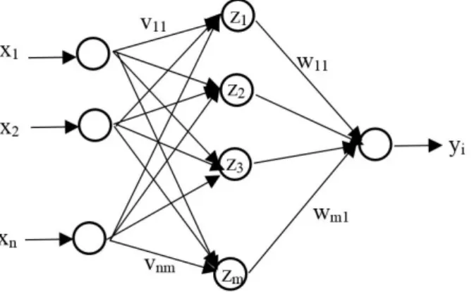
The artificial neural network is a processor made up of neurons. It can learn and store information through the training process. ANNs can handle nonlinearity and, therefore, have a wide application in many disciplines, including the flood hydrograph prediction in hydrology. In general, the three-layer network, as shown in Figure1, is conceptualized in flood hydrograph prediction problems. In such network (see Figure1); the compacted input values (xi) are first entered into the input layer neurons. They are multiplied by the connection weights (vij) and then passed on to the hidden layer neurons. Each neuron sums all the received weighted information (xivij) and then passes the sum through an activation function to produce an output (zi), which in turn, becomes the input signal for the output layer neuron. The output from each inner layer neuron is multiplied by the related connection weight (wij) and then passed on to the output neuron, which sums all the received signal (ziwij) and passes it through an activation function to produce the network output (yi).
Water 2018, 10, x FOR PEER REVIEW 2 of 13
consuming. When lateral flow becomes significant, the flood prediction is affected by high uncertainty [5]. In addition, numerical solutions of the St. Venant equations require a fair amount of data which is often not available and can encounter convergence and stability problems [2].
In the 1990s, the first applications of the artificial neural networks led to the realization that machine learning methods can handle nonlinear problems efficiently and satisfactorily without being restricted by the mathematical operations of integration and/or differentiation [6]. This even led to the development of new machine learning algorithms in the 1990s and the 2000s, such as harmony search (HS), gene expression programming (GEP), and genetic programming (GP). Machine learning (soft) methods are data driven and do not require substantial data and parameter estimation, as in the case of the distributed physically-based hydrologic models. The important advantages of these models are their relatively simple coding, low computational cost, fast convergence, and adaptiveness to new data [6,7].
Flood hydrograph predictions are performed using several soft computing methods, such as the artificial neural network (ANN) [8], the genetic algorithm (GA) [9,10], and the Fuzzy logic methods [11]. Most recently, the performance of some of the machine learning algorithms against the Variable Parameter Muskingum Model (VPMM) was compared [12]. In this context, it is of considerable interest to investigate how well the machine learning methods work in the real field and this study attempts to answer to the demand presenting real flood hydrograph predictions by the ANN, the GA, the ACO, and the PSO and compares the performances against those of the RCM. The flood hydrographs observed along an equipped branch of Tiber River, central Italy, with significant lateral flow contribution is used for testing the methods. In addition, the study tests the performance of these machine learning methods, based on the NMM, against that of the St. Venant equations by flood routing in an artificial channel having different bed slopes.
2. Material and Methods
2.1. Artificial Neural Network (ANN)
The artificial neural network is a processor made up of neurons. It can learn and store information through the training process. ANNs can handle nonlinearity and, therefore, have a wide application in many disciplines, including the flood hydrograph prediction in hydrology. In general, the three-layer network, as shown in Figure 1, is conceptualized in flood hydrograph prediction problems. In such network (see Figure 1); the compacted input values (xi) are first entered into the
input layer neurons. They are multiplied by the connection weights (vij) and then passed on to the
hidden layer neurons. Each neuron sums all the received weighted information (xivij) and then passes
the sum through an activation function to produce an output (zi), which in turn, becomes the input
signal for the output layer neuron. The output from each inner layer neuron is multiplied by the related connection weight (wij) and then passed on to the output neuron, which sums all the received
signal (ziwij) and passes it through an activation function to produce the network output (yi).
The optimal values of the connection weights can be found by the back propagation algorithm, which minimizes the error function by using the gradient decent method. The minimized error function,E, is expressed by Equation (1), as follows [11]:
E=
p
∑
i
(ti−yi)2 (1) where yi is the network output, ti is the user-specified target output, and p is the number of training patterns.
The connection weights (wij) are updated at each iteration using Equation (2), as follows [11]:
∆wij(n) =α∆wij(n−1)−δ ∂E ∂wij
(2)
where∆wij (n)=wijold−wijnewat the present iteration (n), and∆wij (n−1) =wijold −wijnewat the previous iteration (n−1).δis the learning rate andαis the momentum factor, taking values between 0 and 1. In this study, tangent hyperbolic (tanh) activation function (Equation (3)) was employed.
f(sum) = 2
1+e−2sum −1 (3)
wheresumis the total information received by the neuron. The tangent hyperbolic function is bounded in between−1 and +1 and, therefore, all the values were compacted by Equation (4) into−0.9 and +0.9.
zi= 1.8(x i−xmin) xmax−xmin −0.9 (4)
whereziis the standardized value,xminis the minimum value in the set; andxmaxis the maximum value in the set. Details of ANNs are available in the literature [11].
2.2. Genetic Algorithm (GA)
Genetic algorithm (GA) was developed by Holland [13]. The concept is based on the survival of the fittest. It employs chromosomes, each of which consists of many genes. Each gene stands for a decision variable (or a model parameter) and each chromosome stands for a possible optimal solution. Note that each gene is formed from a string of many 0 and 1 digits. The fitness of a chromosome,F(Ci), in a gene pool, which can contain many chromosomes, is found by Equation (5):
F(Ci) =
f(Ci)
∑N
i=1f(Ci)
(5) whereNis the total number of chromosomes,Ciis theithchromosome,f(Ci)is the functional value of theithchromosome, andF(Ci)is the fitness value of theithchromosome.
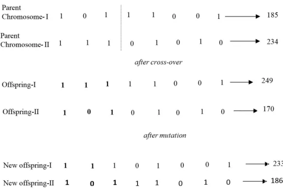
Once the fitness of each chromosome is calculated by Equation (5), then the selection process is performed using either the roulette wheel or the ranking method [14]. Pairing is done after the selection process, then the crossover and mutation operations are applied to each paired chromosome to produce new generations (offsprings). Figure2presents the crossover and mutation operations. As seen, the genes of the first two chromosomes (parent chromosome I and parent chromosome II) were cut from the third digit on the left and interchanged. This yielded a new pair of chromosomes (offspring I and offspring II). The original values 185 and 234 became 249 and 170, respectively. The mutation operation was applied onto the fourth digit from the left of each offspring by simply reversing digit 1 to 0 and digit 0 to 1, respectively. After the mutation operation, 249 and 170 became 233 and 186, respectively. More details on GA can be found in other studies [11,14,15].
Water2018,10, 968 4 of 13
Water 2018, 10, x FOR PEER REVIEW 4 of 13
Figure 2. Example for crossover and mutation operations. 2.3. Particle Swarm Optimization (PSO)
The PSO was developed by Kennedy and Eberhart [16]. The concept is based on the movement of a flock. The individuals in the flock move in search space while adjusting their position and velocity according to the neighboring individuals [17]. The position of an individual, , is adjusted by Equation (6) [18]:
=
+
(6)where xi and viare the particle’s position and velocity vectors, respectively. The particles velocity,
is adjusted by Equation (7) [18]:
=
+
( − ) +
−
(7)where pi is the position of the best candidate solution; pg is the global best position, μis the constriction
coefficient (μ= 1) [19], w is the inertia weight (w = 0.4–0.9) [20], c1 and c2 are the acceleration coefficients
(c1= c2= 2), and r1 and r2 are random values in (0, 1) [21]. The inertia weight is updated by Equation
(8) at each iteration [18]:
=
−
−
(8)where witer is the inertia weight in each iteration, itermax is the maximum number of iterations, and
wmax and wmin are the maximum and minimum inertia weights, respectively. Details of PSO are given
in [16,18].
2.4. Ant Colony Optimization (ACO)
The ACO was developed by Dorigo [22] who wondered how the ants find the shortest path between their nest and a food source. It was found that ants are completely blind but communicate through a chemical tracer called pheromone. Each ant leaves a pheromone on its path. Hence, it is likely that ants will choose the path having the most concentrated pheromone. This suggests that if there are long and short paths between the nest and the food source, then the ants will eventually choose the shortest path.
Figure 2.Example for crossover and mutation operations.
2.3. Particle Swarm Optimization (PSO)
The PSO was developed by Kennedy and Eberhart [16]. The concept is based on the movement of a flock. The individuals in the flock move in search space while adjusting their position and velocity according to the neighboring individuals [17]. The position of an individual,xi, is adjusted by Equation (6) [18]:
xi+1=xi+vi+1 (6) wherexiandviare the particle’s position and velocity vectors, respectively. The particles velocity,vi, is adjusted by Equation (7) [18]:
vi+1=µwvi+c1r1(pi−xi) +c2r2 pg−xi (7) wherepiis the position of the best candidate solution;pgis the global best position,µis the constriction coefficient(µ= 1) [19],wis the inertia weight (w= 0.4–0.9) [20],c1andc2are the acceleration coefficients (c1=c2= 2), andr1andr2are random values in (0, 1) [21]. The inertia weight is updated by Equation (8) at each iteration [18]:
witer=wmax−wmax
−wmin
itermax iter (8)
wherewiteris the inertia weight in each iteration, itermaxis the maximum number of iterations, andwmax andwminare the maximum and minimum inertia weights, respectively. Details of PSO are given in [16,18]. 2.4. Ant Colony Optimization (ACO)
The ACO was developed by Dorigo [22] who wondered how the ants find the shortest path between their nest and a food source. It was found that ants are completely blind but communicate through a chemical tracer called pheromone. Each ant leaves a pheromone on its path. Hence, it is likely that ants will choose the path having the most concentrated pheromone. This suggests that if there are long and short paths between the nest and the food source, then the ants will eventually choose the shortest path.
The probability that optionLi(j)path is chosen at cyclekand iterationt(Pi(j)(k,t)) can be computed by Equation (9) [23]: Pi(j)(k, t) = h Pi(j)(t) iαh µi(j)(t) iβ ∑Li(j) h Pi(j)(t) iαh µi(j)(t) iβ (9)
wherePi(j)(t)is the pheromone concentration associated with optionLi(j)at iteration t;µi(j)=Li(j)/ci(j)is the heuristic factor which favors options having smaller local costs;ci(j)is the set of costs associated with optionsLi(j). αandβare the exponents controlling the relative importance of pheromone and local heuristic factor, respectively.
The pheromone trail is updated using Equation (10) [23]:
Pi(j)(t+1) =δPi(j)(t) +∆Pi(j) (10) where ∆Pi(j) is the change in pheromone concentration associated with option Li(j) and δ is the pheromone persistence coefficient (δ< 1). Employingδhas many advantages, such as the greater exploration of the search space, avoidance of premature convergence and costly solutions. More details of ACO algorithm can be found elsewhere [22,23].
2.5. Data and Catchment
The models were applied to predict real event-based flood hydrographs (Table 1). The hydrographs were recorded along an equipped branch of Tiber River, central Italy (see Figure3). Santa Lucia station is the upstream station and Ponte Felcino station is the downstream station (Figure3). Santa Lucia and Ponte Felcino stations have about 935 km2and 2035 km2drainage areas, respectively. The distance between these two stations is 45 km and the wave travel time of the flood events, as presented in Table1, is, on the average, almost 3.5 h. The duration of each event is also presented in Table1.
The ANN model employed the flow stage data recorded at both stations to predict the flow discharge at Ponte Felcino station. Other machine learning models (PSO, ACO; GA), based on the RCM, employed the cross-sectional area data at both stations and flow discharge data at the upstream station to predict the flow discharge at the downstream station. The 4 events, marked as * in Table1, were used for calibrating (training in the case of ANN) the models. Since the data was recorded every half an hour and considering the duration of these events in Table1, the total number of training patterns (input data sets at the calibration stage) amounted to 1012. The total number of data sets used for the validation (testing) stage was 740. More details on the catchment and data can be found in other studies [3,8–10,24].
Table 1.Main characteristics of observed flood events.
Santa Lucia Station Ponte Felcino Station
TL(h) Duration (h) Qb m3/s Qp m3/s Qb m3/s Qp m3/s December 1990 8 418 9 404 2 98 January 1994 35 108 50 241 3 122 May 1995 * 4 71 8 138 4 217 January 1997 * 18 120 36 225 3 77 June 1997 * 5 345 10 449 5 114 January 2003 24 58 50 218 3 150 February 2004 * 22 91 55 276 3 98
WaterWater 20182018,10, , 96810, x FOR PEER REVIEW 6 of 13 6 of 13
Figure 3. Tiber River Basin at Ponte Felcino gage site.
3. Results and Discussion
3.1. Real Hydrograph Predictions
Flow stage data measured every half an hour at Santa Lucia (upstream station) and Ponte Felcino (downstream station) constituted the input vector of the network, while the flow discharge measured at Ponte Felcino station was the target output. Thus, the network contained 2, 7, and 1 neurons in the input, hidden, and output layers, respectively. The ANN model was trained with 4 events, marked as * in Table 1 and the total number of training patterns was 1012. The ANN model was trained with
δ = 0.04, α = 0.02 and 3000 iterations. The network, by the back propagation algorithm, found the optimal values of the connection weights by minimizing the following objective function:
=
−
(11)where N is the number of observations, is the observed discharge at the downstream station, and is the model-predicted downstream station discharge.
Thetrained ANN model was then employed to predict hydrographs of other three events (December 1990, January 1994, and January 2003 in Table 1). Considering the duration of these events (see Table 1), the total of data sets used in the testing stage was 740. Figure 4 shows the predicted hydrographs, where the performance of ANN was tested against that of the rating curve method (RCM) developed by Moramarco et al. [24] who proposed the relation given by Equation (12):
( ) =
( )
( − )
( − ) +
(12)where Qu is the upstream discharge; Qd is the downstream discharge; Au is the upstream cross-sectional flow area; Ad is the downstream cross-sectional flow area; Tl is the wave travel time; and
Figure 3.Tiber River Basin at Ponte Felcino gage site.
3. Results and Discussion
3.1. Real Hydrograph Predictions
Flow stage data measured every half an hour at Santa Lucia (upstream station) and Ponte Felcino (downstream station) constituted the input vector of the network, while the flow discharge measured at Ponte Felcino station was the target output. Thus, the network contained 2, 7, and 1 neurons in the input, hidden, and output layers, respectively. The ANN model was trained with 4 events, marked as * in Table1and the total number of training patterns was 1012. The ANN model was trained with δ= 0.04,α= 0.02 and 3000 iterations. The network, by the back propagation algorithm, found the optimal values of the connection weights by minimizing the following objective function:
E= N
∑
i=1 Qobsd −Qmodeld 2 (11)whereNis the number of observations, Qobs
d is the observed discharge at the downstream station, andQmodeld is the model-predicted downstream station discharge.
The trained ANN model was then employed to predict hydrographs of other three events (December 1990, January 1994, and January 2003 in Table1). Considering the duration of these events (see Table1), the total of data sets used in the testing stage was 740. Figure4shows the predicted hydrographs, where the performance of ANN was tested against that of the rating curve method (RCM) developed by Moramarco et al. [24] who proposed the relation given by Equation (12):
Qd(t) =α Ad(t) Au(t−Tl)
Qu(t−Tl) +β (12)
where Qu is the upstream discharge; Qd is the downstream discharge; Au is the upstream cross-sectional flow area;Adis the downstream cross-sectional flow area;Tlis the wave travel time; andαandβare the model parameters, estimated using the same relation, given by Equation (12), for the base flow and peak flow cases [3].
The other methods (GA, PSO, and ACO) were also tested against the RCM. These optimization methods, using the same flow hydrographs (the ones used in the training of the ANN) and by minimizing the same error function (Equation (11)) found the optimal values of the RCM parameters. We herein named them accordingly. For example, when the optimal values of the RCM are found using the GA method, we called it GA_RCM model. In the GA_RCM modeling, 80 chromosomes, 80% cross-over rate, and 4% mutation rate were used. The search space was (−3, 3) and (−10, 10) forα andβ, respectively. It took 4200, 4600 and 6000 iterations for ACO_RCM, GA_RCM and SPO_RCM, respectively, to reach the optimum solutions. Table2presents the optimum values obtained by these methods.
Table 2.Optimal values of the Rating Curve Method parameters.
Algorithm α β
GA 1.22 −5.86 PSO 1.20 −5.90 ACO 1.23 −5.84
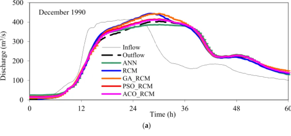
As seen in Figure4, the machine learning models simulated observed hydrographs satisfactorily. They captured the rising and recession limbs, and peak rates with no delay. Table 3summarizes the percentage errors for predicting the peak rates and time to peaks. The negative sign means underestimation for the peak rate and early capturing of the peak rate for the timing. As seen, the models made around 5% (or less) error in predicting the peak rates. This error was around 10% for the classical RCM model. The machine learning methods captured the timing of the peaks with less than 1% error, while it was around 5% for the RCM. Also, the mean absolute error (MAE) and the root mean square error (RMSE) values for each run in Figure4were presented in Table3. As seen, the ANN, the GA_RCM and the ACO_RCM models produced, on average, around 7 m3/s MAE and 9 m3/s RMSE values. These values are, on average, MAE = 11 m3/s and RMSE = 13 m3/s for the PSO_RCM model. The RCM made high errors as 13 m3/s MAE and 17 m3/s RMSE.
Note that the classical RCM needs to estimate differentαandβparameters for each event for the same river reach [8]. On the contrary, herein only a single set of parameters was calibrated by the machine learning algorithms for the same river reach having different inflow flood hydrographs.
Tayfur et al. [8] proposed that ANNs are good interpolators but they cannot be used for the extrapolation purposes. That is, when they are trained by low peak hydrographs they cannot predict high peak ones. On the other hand, Tayfur et al. [10] showed that GA_RCM does not have this shortcoming of the ANN.
Water 2018, 10, x FOR PEER REVIEW 7 of 13
and are the model parameters, estimated using the same relation, given by Equation (12), for the base flow and peak flow cases [3].
The other methods (GA, PSO, and ACO) were also tested against the RCM. These optimization methods, using the same flow hydrographs (the ones used in the training of the ANN) and by minimizing the same error function (Equation (11)) found the optimal values of the RCM parameters. We herein named them accordingly. For example, when the optimal values of the RCM are found using the GA method, we called it GA_RCM model. In the GA_RCM modeling, 80 chromosomes, 80% cross-over rate, and 4% mutation rate were used. The search space was (−3, 3) and (−10, 10) for
α and β, respectively. It took 4200, 4600 and 6000 iterations for ACO_RCM, GA_RCM and SPO_RCM, respectively, to reach the optimum solutions. Table 2 presents the optimum values obtained by these methods.
Table 2. Optimal values of the Rating Curve Method parameters.
Algorithm α β
GA 1.22 −5.86 PSO 1.20 −5.90 ACO 1.23 −5.84
As seen in Figure 4, the machine learning models simulated observed hydrographs satisfactorily. They captured the rising and recession limbs, and peak rates with no delay. Table 3 summarizes the percentage errors for predicting the peak rates and time to peaks. The negative sign means underestimation for the peak rate and early capturing of the peak rate for the timing. As seen, the models made around 5% (or less) error in predicting the peak rates. This error was around 10% for the classical RCM model. The machine learning methods captured the timing of the peaks with less than 1% error, while it was around 5% for the RCM. Also, the mean absolute error (MAE) and the root mean square error (RMSE) values for each run in Figure 4 were presented in Table 3. As seen, the ANN, the GA_RCM and the ACO_RCM models produced, on average, around 7 m3/s MAE and
9 m3/s RMSE values. These values are, on average, MAE = 11 m3/s and RMSE = 13 m3/s for the
PSO_RCM model. The RCM made high errors as 13 m3/s MAE and 17 m3/s RMSE.
Note that the classical RCM needs to estimate different αand β parameters for each event for the same river reach [8]. On the contrary, herein only a single set of parameters was calibrated by the machine learning algorithms for the same river reach having different inflow flood hydrographs.
Tayfur et al. [8] proposed that ANNs are good interpolators but they cannot be used for the extrapolation purposes. That is, when they are trained by low peak hydrographs they cannot predict high peak ones. On the other hand, Tayfur et al. [10] showed that GA_RCM does not have this shortcoming of the ANN.
(a) 0 100 200 300 400 500 0 12 24 36 48 60 Discharge (m 3/s) Time (h) December 1990 Inflow Outflow ANN RCM GA_RCM PSO_RCM ACO_RCM Figure 4.Cont.
Water2018,10, 968 8 of 13
Water 2018, 10, x FOR PEER REVIEW 8 of 13
(b)
(c)
Figure 4. Flood Hydrograph simulations: (a) December 1990; (b) January 1994; and (c) January 2003.
Table 3. Error measures (EQp: % error in peak discharge, and ETp: % error in time to peak).
December 1990 January 1994 January 2003 EQp (%) ANN −5 4 5 GA_RCM 10 −3 −1 PSO_RCM 2 −4 10 ACO_RCM 2 −3 −2 RCM 10 10 12 ETp (%) ANN 0 0 0 GA_RCM 0 2 0 PSO_RCM 0 2 −2 ACO_RCM 0 2 0 RCM −10 −2 4 MAE (m3/s) Mean ANN 8.5 5.6 8.7 7.6 GA_RCM 12.7 4.4 4.7 7.3 PSO_RCM 6.2 12.0 15.4 11.2 ACO_RCM 4.6 3.5 9.1 5.7 RCM 10.4 13.2 14.9 12.8 RMSE (m3/s) Mean 0 50 100 150 200 250 300 350 18 24 30 36 42 48 54 Discharge (m 3/s) Time (h) January 1994 Inflow Outflow ANN-Model RCM-Model PSO_RCM GA_RCM ACO_RCM 0 40 80 120 160 200 240 280 0 24 48 72 96 120 Discharge (m 3/s) Time (h) January 2003 InflowOutflow
ANN RCM PSO_RCM GA_RCM ACO_RCM
Figure 4.Flood Hydrograph simulations: (a) December 1990; (b) January 1994; and (c) January 2003.
Table 3.Error measures (EQp: % error in peak discharge, andETp: % error in time to peak).
December 1990 January 1994 January 2003 EQp(%) ANN −5 4 5 GA_RCM 10 −3 −1 PSO_RCM 2 −4 10 ACO_RCM 2 −3 −2 RCM 10 10 12 ETp(%) ANN 0 0 0 GA_RCM 0 2 0 PSO_RCM 0 2 −2 ACO_RCM 0 2 0 RCM −10 −2 4 MAE (m3/s) Mean ANN 8.5 5.6 8.7 7.6 GA_RCM 12.7 4.4 4.7 7.3 PSO_RCM 6.2 12.0 15.4 11.2 ACO_RCM 4.6 3.5 9.1 5.7 RCM 10.4 13.2 14.9 12.8 RMSE (m3/s) Mean ANN 10.3 7.0 9.2 8.8 GA_RCM 15.7 7.1 6.1 9.6 PSO_RCM 8.5 14.7 17.6 13.6 ACO_RCM 6.4 6.3 9.8 7.5 RCM 16.2 17.7 15.9 16.6
3.2. Hydrograph Predictions in an Artificial Channel Reach
For this purpose, we considered flood routing in an artificial channel reach of 38 km, with a rectangular cross-section of 40 m width and the Manning roughness value of 0.032. The GA, PSO and ACO methods were used to find the optimal values of the parameters (K,x,m) of the nonlinear Muskingum (NMM) flood routing method, which can be expressed as follows [25]:
I(t)−O(t) = dS(t)
dt (13)
S(t) =K[xI(t) + (1−x)O(t)]m (14) whereI(t),O(t)andS(t), respectively, denote the inflow, outflow and reach storage at timet;andx andK, respectively, denote the parameters of the method known as the weighing parameter and flood wave travel time between inlet and outlet sections of the routing reach, andmis the exponent of the weighted discharge. We herein name the models GA_NMM, PSO_NMM, and ACO_NMM. For example, if the parameters of the NMM are found by applying the GA method, then it is called herein as GA_NMM model.
The performance of the ANN, GA_NMM, ACO_NMM and PSO_NMM methods were tested against that of the numerical solutions of the physically-based equations of one-dimensional St. Venant equations: ∂A ∂t + ∂Q ∂x =ql (15) ∂Q ∂t + ∂(Qu) ∂x +gA ∂h ∂x =gA So−Sf (16) whereAis the cross-sectional flow area,Qis the flow rate,qlis the unit lateral flow,gis the gravitational acceleration,uis the flow velocity,Sois the channel bed slope andSfis friction slope (energy gradient). These equations are well established in the literature [1,2].
By the GA_NMM, ACO_NMM and PSO_NMM, the optimal values of the coefficients (K, x, and m) of the NMM model (see Equations (13) and (14)) were found by minimizing MAE function:
MAE= 1 N N
∑
i=1 |QN MM−QSV| (17)whereQNMMis the computed flow discharge by the NMM (Equations (13) and (14)), andQSVis the computed flow discharge by the St. Venant (SV) equations (Equations (15) and (16)).
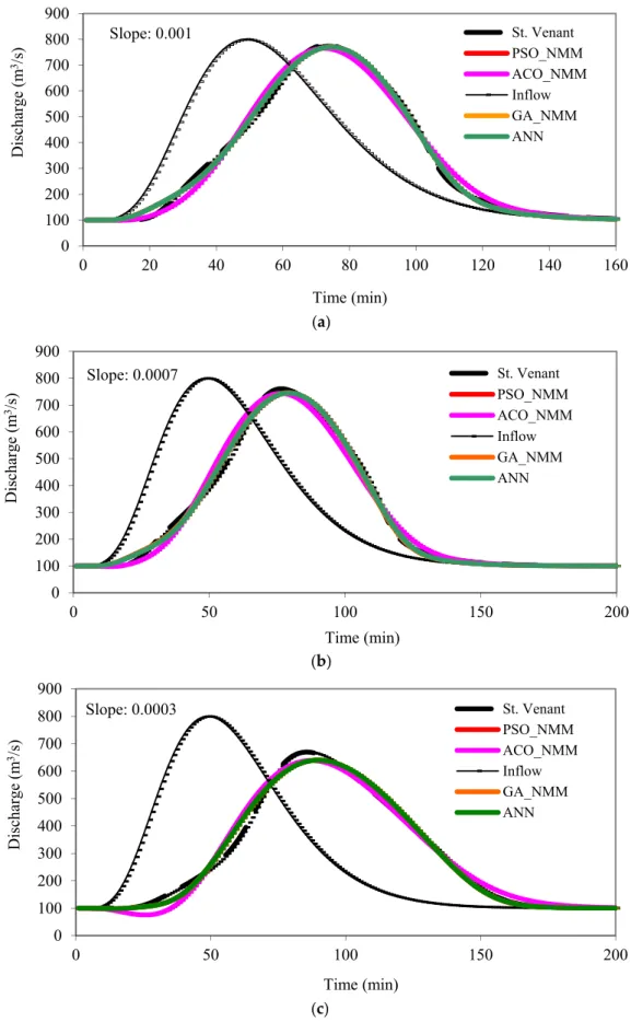
The inflow hydrograph, similar to the one shown in Figure5, with maximum peak of 900 m3/s, time to peak of 26 h, and base flow rate of 120 m3/s, was routed in the same channel reach having three different bed slopes (So: 0.001, 0.0007, and 0.0003) by the St. Venant equations and the generated outflow hydrographs were used to obtain the optimal values of the NMM by the machine learning methods. The search space was 0–1 forK, 0–0.5 forxand 1–3 form. It took 3000, 3600 and 4000 iterations for GA, ACO and SPO, respectively, to reach the optimum solutions. Table4presents the optimal values of NMM. Figure5presents the validation runs for a different inflow hydrograph having 100 m3/s base flow rate, 800 m3/s peak discharge, and 50 h for the time to peak. The inflow hydrograph was routed three times in the same channel reach having different bed slopes. Note that a single set of parameter values given in Table4were obtained for the same reach having different bed slopes. Also, note that with the same hydrographs that are used for the calibration of the other methods (GA_NMM, PSO_NMM, and ACO_NMM). In the training stage of the ANN, 5000 iterations and 0.04 forδandα were employed.
Water2018,10, 968 10 of 13
Water 2018, 10, x FOR PEER REVIEW 10 of 13
methods (GA_NMM, PSO_NMM, and ACO_NMM). In the training stage of the ANN, 5000 iterations and 0.04 for δ and α were employed.
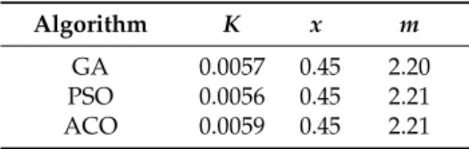
Table 4. Optimal values of the Nonlinear Muskingum Model parameters.
Algorithm K x m
GA 0.0057 0.45 2.20 PSO 0.0056 0.45 2.21 ACO 0.0059 0.45 2.21
As seen in Figure 5, the machine learning algorithms can successfully be employed for simulating flood hydrographs. They are able to capture the peak discharge values as well as the timing of the peaks and the flood volumes, and the rising and recession limbs of the hydrographs. Their performance is as good as that of the St. Venant model. When Perumal et al. [12] investigated the performance of some of the machine learning algorithms against that of the VPMM using a compound channel reach of 40 km, they calibrated the NMM model parameters separately for each river reach having different bed slopes. Herein, a single set of parameters was obtained for the same river reach having different bed slopes.
(a) (b) 0 100 200 300 400 500 600 700 800 900 0 20 40 60 80 100 120 140 160 Discharge (m 3/s) Time (min) Slope: 0.001 St. Venant PSO_NMM ACO_NMM Inflow GA_NMM ANN 0 100 200 300 400 500 600 700 800 900 0 50 100 150 200 Discharge (m 3/s) Time (min) Slope: 0.0007 St. Venant PSO_NMM ACO_NMM Inflow GA_NMM ANN
Water 2018, 10, x FOR PEER REVIEW 11 of 13
(c)
Figure 5. Hydrograph simulations: (a) Slope = 0.001, (b) Slope = 0.0007, and (c) Slope = 0.0003.
Any nonlinear search method, such as the multivariate Newton’s method, could be used to obtain the optimal values of the NMM. However, the machine learning methods are basically a nonlinear search and optimization methods that do not rely on the mathematical properties of a function, such as the continuity and the differentiability. Hence, they can be used in solving nonlinear, nonconvex, and multimodal problems for which deterministic search techniques incur difficulty or fail completely. Furthermore, the machine learning methods have advantages such as the simple coding, low computational cost, fast convergence, and adaptiveness to new data. The machine learning methods including the recurrent neural networks and neuro-fuzzy networks can also be employed for multi-step-ahead flood and water level forecasting purposes [26,27].
4. Concluding Remarks
The following conclusions are drawn from this study:
1. Machine learning methods can make good predictions of flood hydrographs, using substantially less data, such as easily measurable flow stage. Hence, they can be conveniently adopted for predictions in poorly gauged stations, which is the common case in developing countries. The machine learning methods can be employed in conjunction with the physically based models employing the data acquired by newly developed technologies (the remote sensing, satellite). 2. It is proved by using field data that machine learning algorithms, such as GA, ACO, and PSO
are optimization methods without being considered black box models. Since there is a mathematical relation, they both have interpolation and extrapolation capabilities. One more advantage of these models is that one can propose a new equation, such as RCM, provided that it physically makes sense, and by one of these methods, one can find optimal values of the coefficients and exponents of the equation. These methods are robust and efficient and have low computational cost and fast convergence.
3. It is shown that RCM model, whose parameters were optimized by the machine learning algorithm, (GA-RCM, PSO_RCM and ACO_RCM), was able to successfully predict event-based individual storm hydrographs having a different magnitude of lateral inflows at the investigated river reach of the Upper Tiber River basin in central Italy. It closely captured the trends, time to peak, and peak rates of the storms with on average, less than 1% and 5% errors, respectively.
4.
Likewise, the machine learning-based nonlinear Muskingum models (NMM) can successfully be employed for predicting flood hydrographs. They are able to capture the peak discharge values as well as the timing of the peaks and the flood volumes, and the rising and recession limbs of the hydrographs. Their performance is as good as the St. Venant model.0 100 200 300 400 500 600 700 800 900 0 50 100 150 200 Discharge (m 3/s) Time (min) Slope: 0.0003 St. Venant PSO_NMM ACO_NMM Inflow GA_NMM ANN
Table 4.Optimal values of the Nonlinear Muskingum Model parameters.
Algorithm K x m
GA 0.0057 0.45 2.20 PSO 0.0056 0.45 2.21 ACO 0.0059 0.45 2.21
As seen in Figure5, the machine learning algorithms can successfully be employed for simulating flood hydrographs. They are able to capture the peak discharge values as well as the timing of the peaks and the flood volumes, and the rising and recession limbs of the hydrographs. Their performance is as good as that of the St. Venant model. When Perumal et al. [12] investigated the performance of some of the machine learning algorithms against that of the VPMM using a compound channel reach of 40 km, they calibrated the NMM model parameters separately for each river reach having different bed slopes. Herein, a single set of parameters was obtained for the same river reach having different bed slopes.
Any nonlinear search method, such as the multivariate Newton’s method, could be used to obtain the optimal values of the NMM. However, the machine learning methods are basically a nonlinear search and optimization methods that do not rely on the mathematical properties of a function, such as the continuity and the differentiability. Hence, they can be used in solving nonlinear, nonconvex, and multimodal problems for which deterministic search techniques incur difficulty or fail completely. Furthermore, the machine learning methods have advantages such as the simple coding, low computational cost, fast convergence, and adaptiveness to new data. The machine learning methods including the recurrent neural networks and neuro-fuzzy networks can also be employed for multi-step-ahead flood and water level forecasting purposes [26,27].
4. Concluding Remarks
The following conclusions are drawn from this study:
1. Machine learning methods can make good predictions of flood hydrographs, using substantially less data, such as easily measurable flow stage. Hence, they can be conveniently adopted for predictions in poorly gauged stations, which is the common case in developing countries. The machine learning methods can be employed in conjunction with the physically based models employing the data acquired by newly developed technologies (the remote sensing, satellite). 2. It is proved by using field data that machine learning algorithms, such as GA, ACO, and PSO are
optimization methods without being considered black box models. Since there is a mathematical relation, they both have interpolation and extrapolation capabilities. One more advantage of these models is that one can propose a new equation, such as RCM, provided that it physically makes sense, and by one of these methods, one can find optimal values of the coefficients and exponents of the equation. These methods are robust and efficient and have low computational cost and fast convergence.
3. It is shown that RCM model, whose parameters were optimized by the machine learning algorithm, (GA-RCM, PSO_RCM and ACO_RCM), was able to successfully predict event-based individual storm hydrographs having a different magnitude of lateral inflows at the investigated river reach of the Upper Tiber River basin in central Italy. It closely captured the trends, time to peak, and peak rates of the storms with on average, less than 1% and 5% errors, respectively. 4. Likewise, the machine learning-based nonlinear Muskingum models (NMM) can successfully be
employed for predicting flood hydrographs. They are able to capture the peak discharge values as well as the timing of the peaks and the flood volumes, and the rising and recession limbs of the hydrographs. Their performance is as good as the St. Venant model.
5. The use of machine learning for discharge prediction is essential for hydrological practices, considering that often, for many river gauging sites, the maintenance is missing, and streamflow
Water2018,10, 968 12 of 13
measurements are more and more limited to few strategic gauged river sections. The option to monitor only water levels at gage sites makes these approaches very appealing for their capability to relate, by RCM, local stages and remote discharge.
Author Contributions:G.T. and V.P.S. initiated the research. T.M. and S.B. provided the field data. G.T. carried out the simulations and wrote the first rough draft of the manuscript. V.P.S., T.M. and S.B. analyzed the results, made feedbacks and revised the paper.
Funding:This research received no external funding.
Acknowledgments:The authors wish to thank the Department of Environment, Planning, and Infrastructure of Umbria Region for providing Tiber River data.
Conflicts of Interest:The authors declare no conflict of interest.
References
1. Henderson, F.M.Open Channel Flow; MacMillan: New York, NY, USA, 1966.
2. Chaudhry, M.H.Open-Channel Flow; Prentice Hall: Upper Saddle River, NJ, USA, 1993.
3. Barbetta, S.; Franchini, M.; Melone, F.; Moramarco, T. Enhancement and comprehensive evaluation of the Rating Curve Model for different river sites.J. Hydrol.2012,464–465, 376–387. [CrossRef]
4. Kundzewicz, Z.W.; Napiorkowski, J.J. Nonlinear models of dynamic hydrology.Hydrol. Sci. J.1986,312, 163–185. [CrossRef]
5. Barbetta, S.; Moramarco, T.; Perumal, M. A Muskingum-based methodology for river discharge estimation and rating curve development under significant lateral inflow conditions. J. Hydrol. 2017,554, 216–232. [CrossRef]
6. ASCE Task Committee. Artificial neural networks in hydrology. I: Preliminary concepts.J. Hydrol. Eng.2000, 5, 115–123.
7. Tayfur, G. Modern optimization methods in water resources planning, engineering and management.Water Resour. Manag.2017,31, 3205–3233. [CrossRef]
8. Tayfur, G.; Moramarco, T.; Singh, V.P. Predicting and forecasting flow discharge at sites receiving significant lateral inflow.Hydrol. Process.2007,21, 1848–1859. [CrossRef]
9. Tayfur, G.; Moramarco, T. Predicting hourly-based flow discharge hydrographs from level data using genetic algorithms.J. Hydrol.2008,352, 77–93. [CrossRef]
10. Tayfur, G.; Barbetta, S.; Moramarco, T. Genetic algorithm-based discharge estimation at sites receiving lateral inflows.J. Hydrol. Eng.2009,14, 463–474. [CrossRef]
11. Tayfur, G.Soft Computing in Water Resources Engineering: Artificial Neural Networks, Fuzzy Logic, and Genetic Algorithm; WIT Press: Southampton, UK, 2012.
12. Perumal, M.; Tayfur, G.; Rao, C.M.; Gurarslan, G. Evaluation of a physically based quasi-linear and a conceptually based nonlinear Muskingum methods.J. Hydrol.2017,546, 437–449. [CrossRef]
13. Holland, J.H.Adaptation in Natural and Artificial Systems; University of Michigan Press: Ann Arbor, MI, USA, 1975. 14. Sen, Z.Genetic Algorithm and Optimization Methods; Su Vakfı Yayınları: Istanbul, Turkey, 2004. (In Turkish) 15. Goldberg, D.E. Computer-Aided Gas Pipeline Operation Using Genetic Algorithms and Rule Learning.
Ph.D. Thesis, University of Michigan, Ann Arbor, MI, USA, 1983.
16. Kennedy, J.; Eberhart, R. Particle swarm optimization. In Proceedings of the IEEE International Conference on Neural Networks, Perth, Australia, 27 November–1 December 1995; pp. 1942–1948. [CrossRef]
17. Kumar, D.N.; Reddy, M.J. Multipurpose reservoir operation using particle swarm optimization.J. Water Resour. Plan. Manag.2007,133, 192–201. [CrossRef]
18. Shourian, M.; Mousavi, S.J.; Tahershamsi, A. Basin-wide water resources planning by integrating PSO algorithm and MODSIM.Water Resour. Manag.2008,22, 1347–1366. [CrossRef]
19. Ostadrahimi, L.; Marino, M.A.; Afshar, A. Multi-reservoir operation rules: Multi-swarm PSO-based optimization approach.Water Resour. Manag.2012,26, 407–427. [CrossRef]
20. Moghaddam, A.; Behmanesh, J.; Farsijani, A. Parameters estimation for the new four-parameter nonlinear Muskingum model using the particle swarm optimization. Water Resour. Manag. 2016,30, 2143–2160. [CrossRef]
21. Afshar, A.; Shojaei, N.; Sagharjooghifarahani, M. Multiobjective calibration of reservoir water quality modeling using multiobjective particle swarm optimization (MOPSO).Water Resour. Manag. 2013, 27, 1931–1947. [CrossRef]
22. Dorigo, M. Optimization, Learning and Natural Algorithms. Ph.D. Thesis, Dipartimento di Elettronica, Politecnico di Milano, Milano, Italy, 1992. (In Italian)
23. Dorigo, M.; Maniezzo, V.; Colorni, A. Ant system: Optimization by a colony of cooperating agents.IEEE Trans. Syst. Man Cybern. Part B Cybern.1996,26, 29–41. [CrossRef] [PubMed]
24. Moramarco, M.; Barbetta, S.; Melone, F.; Singh, V.P. Relating local stage and remote discharge with significant lateral inflow.J. Hydrol. Eng.2005,10, 58–69. [CrossRef]
25. Chow, V.T.; Maidment, D.R.; Mays, L.W.Applied Hydrology; McGraw-Hill: New York, NY, USA, 1988. 26. Chang, F.J.; Chiang, Y.M.; Ho, Y.H. Multi-step-ahead flood forecasts by neuro-fuzzy networks with effective
rainfall-runoff patterns.J. Flood Risk Manag.2015,8, 224–236. [CrossRef]
27. Chang, F.J.; Chen, P.A.; Lu, Y.R.; Huang, E.; Chang, K.Y. Real-time multi-step-ahead water level forecasting by recurrent neural networks for urban flood control.J. Hydrol.2014,517, 836–846. [CrossRef]
© 2018 by the authors. Licensee MDPI, Basel, Switzerland. This article is an open access article distributed under the terms and conditions of the Creative Commons Attribution (CC BY) license (http://creativecommons.org/licenses/by/4.0/).