Longitudinal Mediation Analysis Using Natural E
ff
ect
Models
Murthy N. Mittinty∗1and Stijn Vansteelandt†2,3
1School of Public Health, The University of Adelaide, South Australia, 5000 Australia. Phone:+61 8 8303961 2
Department of Applied Mathematics, Computer Science and Statistics, Krijslaan 281, Gent University, Gent , Belgium.
3
Department of Medical Statistics, London School of Hygiene and Tropical Medicine, London, UK
Abstract
Mediation analysis is concerned with the decomposition of the total effect of an ex-posure on an outcome into the indirect effect through a given mediator, and the remaining direct effect. This is ideally done using longitudinal measurements of the mediator, as these capture the mediator process more finely. However, longitudinal measurements pose chal-lenges for mediation analysis. This is because the mediators and outcomes measured at a given time-point can act as confounders for the association between mediators and out-comes at a later time-point; these confounders are themselves affected by the prior exposure and outcome. Such post-treatment confounding cannot be dealt with using standard meth-ods (e.g. generalised estimating equations). Analysis is further complicated by the need for so-called cross-world counterfactuals to decompose the total effect. This article addresses these challenges. In particular, we introduce so-called natural effect models, which parame-terise the direct and indirect effect of a baseline exposure w.r.t. a longitudinal mediator and outcome. These can be viewed as a generalisation of marginal structural models to enable effect decomposition. We introduce inverse probability weighting techniques for fitting these models, adjusting for (measured) time-varying confounding of the mediator-outcome association. Application of this methodology uses data from the Millennium Cohort Study, UK.
1
Introduction
Mediation analyses are ideally based on longitudinal measurements of the mediator. These rep-resent the entire mediator process better than a single assessment of the mediator. At least in principle, they should thus better allow to capture the extent to which exposure influences out-come by affecting that mediator process, which may in turn influence outout-come. In spite of this,
∗
†
developments on counterfactual-based mediation analyses have rarely considered longitudinal mediators. This is largely related to the difficulties of identifying (natural) direct and indirect ef-fect in the presence of confounders of the mediator-outcome association, which are themselves affected by the exposure (1, 2). Such confounders are essentially guaranteed to exist in longi-tudinal mediation analyses because the association between mediator and outcome at a given point in time is typically confounded by the history of mediators and outcomes (amongst other things), which are often affected by the exposure.
In view of this, early work on longitudinal counterfactual-based mediation analysis (3) consid-ered settings where such time-varying confounders could be assumed absent. More recent work (4, 5) has shifted the focus from natural direct and indirect effect (or more specifically, path-specific effects) to so-called interventional direct and indirect effect, which can be identified under weaker conditions (2, 6, 7), but do not always enable decomposition of the total effect into direct and indirect pathways. By relying on a general identification theory for path-specific effects by Shpitser (8), Vansteelandt et al. (9) showed how to decompose the effect of a point ex-posure on an arbitrary outcome into the path-specific effect via the mediator (i.e., the combined effect due to the exposure directly influencing one of the mediators, which then in turn influences the outcome) versus the remaining direct effect. Assuming that the data-generating mechanism can be represented by a nonparametric structural equation model with independent errors, and assuming that there is no unmeasured confounding of the exposure-mediator, exposure-outcome and mediator-outcome associations, they used strategies analogous to g-computation to estimate these effects from observational data. Like other g-computation estimators, their results can be very sensitive to model misspecification, do not readily allow for testing for the presence of direct and indirect effect, and can be difficult to report when the exposure takes on more than two levels or the outcome is repeatedly measured over time (for then one may need to report a direct and indirect effect for each exposure level and w.r.t. each outcome separately).
To accommodate this, this paper extends the class of natural effect models previously introduced by Lange et al.(10) and Vansteelandt et al.(11) to longitudinal mediation analysis. Natural effect models generalise marginal structural models to enable effect decomposition. Building on (5) we propose inverse probability weighting strategies for fitting these models, which are much less demanding in terms of modelling assumptions than g-computation estimators, are relatively easy to perform using standard software, and avoid extrapolation when subjects with different levels of exposure or mediator are very different in their observed background characteristics. We illustrate the proposal with an analysis of the effect of socio-economic status on child mental health using data from the Millennium Cohort Study (UK) and the extent to which this effect is mediated by maternal psychological distress.
2
E
ff
ect decomposition into direct and indirect e
ff
ect
2.1 Decomposition in single mediator and single exposure setting
Notation, definition and identification. In the counterfactual framework, causal effects are
de-fined by contrasting counterfactual outcomes under different exposure settings. For example, the total causal effect of a binary exposure (A = 1 for exposed, A = 0 for unexposed) on an outcome,Y, is obtained by comparingY1andY0, withYathe counterfactual outcome that would
have been observed ifA were set, possibly contrary to the fact, toa. The population average effect then can be quantified in terms of a mean difference,E{Y1−Y0}, or when the outcome is binary, alternatively as the relative risk P{Y1 = 1}/P{Y0 = 1}. Following the causal inference literature (12, 13, 14) we will further describe direct and indirect effect via a given mediator M
observed ifAwas set toaandMwas set to the value it would have taken ifAwas set toa∗. In particular we will compareYa,Ma∗ withYa∗,Ma∗ to express the direct effect of changing the expo-sureatoa∗. Such comparison can for instance, be made in terms of an average difference within levels of baseline covariates (L0),E{Ya,Ma∗ −Ya∗,M
a∗|L0}, or marginally, E{Ya,Ma∗ −Ya∗,M
a∗}; as a risk ratio, P{Ya,Ma∗ = 1}/P{Ya∗,Ma∗ = 1}, and so on. Likewise we will compareYa∗,Ma with
Ya∗,M
a∗, to obtain a measure of the indirect effect via the mediator. For example, on the additive
scale, the total causal effect decomposes into the sum of the so-called natural direct effect and indirect effect
E{Y1−Y0}= E{Y1,M0 −Y0,M0}+E{Y1,M1−Y1,M0}
given the composition assumption thatYa,Ma =Ya. The word “natural” refers to the fact that we
have let the mediator take the value it would take naturally when the exposure is set toa. In this one time point setting, nonparametric identification of natural direct and indirect effect is possible by making a set of sufficient conditions, which state that for any value ofa,a∗andm
Ya,m⊥⊥A|L0 (1)
Ya,m⊥⊥M|A=a,L0 (2)
Ma ⊥⊥A|L0 (3)
Ya,m⊥⊥Ma∗|L0 (4)
whereA⊥⊥ B|Cmust be read asAandBare independent conditional onC. Here,Yamdenotes the counterfactual outcome that would have been observed ifAwere set toaandMtom. Con-ditions 1-4 require just the baseline confounders L0 to deconfound (a) the effect of exposure
Aon outcomeY, (b) the effect of mediatorM on outcomeY conditional on exposure; and (c) the effect of the exposure on the mediator. Assumption (4) is stronger because it involves the dependence between counterfactuals at different exposure levels. Assumptions (1)-(4) cannot simultaneously hold when there are confounders of the mediator-outcome association that are affected by the exposure.
Natural effect models. Under conditions 1-4, the natural direct and indirect effect can be
pa-rameterised via so-called natural effect models (10, 11). These express the mean of nested counterfactual outcomes, thereby naturally extending marginal structural models to allow for effect decomposition. For example, suppose that the mean ofYa,Ma∗ obeys
E(Ya,Ma∗)=β0+β1a+β2a
∗+β
3a.a∗ (5)
for alla,a∗. Then,β1captures the direct effect
E{Y1,M0 −Y0,M0}=β1
andβ2+β3captures the indirect effect
E{Y1,M1−Y1,M0}=β2+β3
The effectsβ1andβ2+β3correspond to theA→Yand theA→M→Ypaths, labelled asIand
IIin the directed acyclic graph (DAG) (see Figure 1, left panel). This decomposition of the total causal effect (β1+β2+β3) is not unique (15). In particular, the direct effect can alternatively be defined as
E{Y1,M1−Y0,M1}=β1+β3
and the indirect effect as
A
M
L
0Y
II I IIA
M
L
1Y
I I I II I IIFigure 1: Causal Directed Acyclic Graph with exposure A, mediator M, outcome Y and pre-treatment confounderL0(left) and post treatment confounderL1(right)
It is thus seen that whenβ3 ,0, the direct effect may depend on the natural level at which the mediator is controlled. Finally, note that whena = a∗, then model 5 reduces to the marginal structural model
E(Ya,Ma)=E(Ya)=β0+(β1+β2+β3a)a.
Natural effect models thus generalise marginal structural models to enable effect decomposition. Model 5 is a special case of the wider class of generalised linear natural effect models (10, 11) given by
g{E(Ya,Ma∗|L0)}=βTW(a,a ∗,
L∗0)
where g is a known link function (e.g. the identity, log or logit link) and W(a,a∗,L∗0) is a known vector with components that may depend ona anda∗and (possibly) a set of baseline covariatesL∗0(L∗0 ⊆L0),βthe unknown vector of parameters of interest, for example, in equation 5,W(a,a∗,L0∗) = (1,a,a∗,a.a∗)T. Instead, when one is interested in effect modification by the confounder (L0), then equation 5 can be modified to (10),
E(Ya,Ma∗|L0)=β0+β1a+β2a∗+β3a.a∗+β4L0+β5a.L0+β6a∗L0. (6) The parameters indexing equation 6 represent aspects of conditional direct and indirect effect. Effect modification of the direct and indirect effect by the confounder L0is captured byβ5and β6, respectively.
In applied mediation analyses, some of the mediator-outcome confounders are often affected by the exposure. This generates complex forms of confounding, which are essentially guaranteed to exist in longitudinal mediation analyses (see the next section). In particular, this induces a violation of identification assumptions 2 and 4, thereby rendering the natural direct and indirect effect non-identified without making strong untestable assumptions (16). In such cases, we will focus on the identification of specific path-specific effects (for more details refer to (2)). In particular, we redefine the counterfactual outcomeYa,Ma∗ as expressing the outcome that would be observed if the exposureAwas set toa(so that in particularL1takes on the valueL1a), and
if Mwas set to the value it would take if the exposureAwas set toa∗andL1 was still kept at
L1a; this counterfactual is more carefully denoted Ya,L1a,Ma∗L
1a, a notation which we will avoid
to keep it manageable. In that case, the total effect can still be decomposed, but the direct effect β1 in equation 5 now corresponds to the combination of the paths A → L1 → Y, A → Y and
A →L1 → M →Y (shown asI in Figure 1 right), and the indirect effect,β2+β3corresponds to the pathA→M→Y (shown asIIin Figure 1 right) (2).
3
Extension to point exposure and time-varying mediator
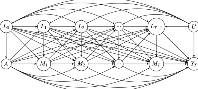
In this paper, we will extend the above framework to longitudinal mediators and outcomes, while still focussing on point exposures. LetT be the number of visits (excluding the baseline visit t=0) on which individuals are measured,t = 1,2,3, ...,T. In particular, suppose that at each of these times we observe data on an outcomeYt, mediators Mt and a vector of covariates
Lt. Figure 2 depicts how they are related over time. Throughout, we will denote the history of
measurements up to timetusing a bar (e.g. Mt = (M1,M2, ...,MT)). We will further assume thatYt may have been influenced by Mt andLt, and that Mt may have been influenced byLt. We are now ready to define the nested counterfactual outcomeYt,a,M
t,a∗ at each time point tas
the outcome that would be observed at timetif, for s = 1, . . . ,T −1, Lswas set to the value we would have observed if the exposure was set toa (and all previous instances ofL and M
to the values we have already set) and Ms was set to the value we would have observed if the
exposure was set to a∗ (and all previous instances of Land M to the values we have already set). Correspondingly, the contrastE[Yt,a,M
t,a∗ −Yt,a∗,Mt,a∗] encodes the path-specific effects on
the outcome at time tof changing the exposure from a toa∗, which captures the effect of A
onYalong all pathways, except those whereAdirectly influences one of the mediatorsMs,s =
1, ...,T. It thus captures the effect of exposure on outcome along any of the pathways in Figure 2
whereAdirectly influences either the outcome, or one of the time-varying confoundersLt, which
may then subsequently affect outcome. The contrast E[Yt,a,M
t,a − Yt,a,Mt,a∗] encodes the
path-specific effects on the outcome at timetof changing the exposure fromatoa∗, as a result ofA
directly influencing one of the mediatorsMs. It thus captures the effect of exposure on outcome
along any of the pathways in Figure 2 where A directly influences one of the time-varying mediatorsMt, which may then subsequently affect outcome. Note that the mediated effect on
which we focus, thus excludes pathways whereby treatment initially influences time-dependent patient characteristics L, which then in turn influence the mediator and thereby the outcome. Those pathways will be attributed to the indirect effect via those patient characteristics. This seems logical from an interpretational point of view, but is also a more fundamental requirement: the effect of treatment transmitted along the combination of all pathways that intercept one or multiple mediators (regardless of where in the causal chain it intercepts these variables) cannot be identified without making overly stringent assumptions (1, 8, 9).
Below we will discuss identification and estimation of the above path-specific effects under the no-unmeasured confounding assumptions implicit in the causal diagram of Figure 2, which is assumed to represent a nonparametric structural equation model with independent errors. In particular as in (9), we will assume that the same set of baseline covariates L0 is sufficient to control for confounding of associations between exposure and outcome, and of exposure and mediator. We will moreover assume that at each timetand each times ≤ t, adjustment for the history A,Ls,Ms−1 suffices to control for confounding of the effect of Ms onYt. Throughout,
we will assume that there is no loss to follow-up and measurement error in the mediators.
3.1 Natural Effect Models for Longitudinal Mediators
Previously reviewed natural effect models can be extended to longitudinal mediators and out-comes. For instance, equation 5 can be extended to accommodate time dependent mediators as follows:
g{E[Yt,a,M
t,a∗]}=α0+α1a+α2a
∗+α
3t+α4t.a+α5t.a∗ (7) for a user-specified link functiong(.). This generalises the marginal structural model
Wheng(.) is the identity link, then according to equation 7 the total effect of a unit increase in the exposure,α1+α2+(α4+α5)t, can be decomposed into direct effect
E{Yt,1,M
t,0−Yt,0,Mt,0}=α1+α4t
and the indirect effect
E{Yt,1,M
t,1−Yt,1,Mt,0}=α2+α5t.
Equation 7 excludes the possibility of mediator-exposure interaction (on the scale of the link functiong(.)). However, such interactions can be allowed in the model by includinga.a∗term in the model.
3.2 Estimation
Here we describe how the coefficients in natural effect models of the form (equation 7) can be estimated for a binary point exposure, a longitudinal outcome, and a longitudinal categorical mediator, using inverse probability weighting. Estimation using natural effect models is not lim-ited to these types of variables but can in principle accommodate arbitrary exposures, mediator and outcomes (e.g. binary, categorical, continuous).
3.2.1 Regression for Exposure
To adjust for confounding of the exposure-mediator and exposure-outcome associations, we will first calculate inverse probability of exposure weights. Assuming
logit(P[A=1|L0=l0]) = γ0+γ1l0, (8)
estimated probabilities ( ˆpi) for each individualican be obtained as ˆpi =expit( ˆγ0+γˆ1l0i). The
weight for theithindividual is thenwai = p1ˆ
i ifAi=1 andw
a i =
1
(1−pˆi) ifAi =0.
3.2.2 Regression for the mediators
To decompose the total effect into path-specific effects, while adjusting for confounding of the mediator-outcome associations, we will next calculate mediator weights. For a categorical me-diator Mt with possible valuesk = 0, ...,K, we will fit multinomial models at each time point. For the mediator at the first time point, we may for instance fit the multinomial logistic model:
pr[M1 =k|A=a,L1=l1] = exp(δ0k+δ1ka+δ2kl1) 1+PK l=1exp(δ0l+δ1la+δ2ll1) ,k=1,2, ...,K pr[M1=0|A=a,L1=l1] = 1 1+PK l=1exp(δ0l+δ1la+δ2ll1) (9)
and then subsequently for all later time points:
pr[Mt =k|A=a,Mt−1 =mt−1,Lt =lt] = exp(δ0k+δ1ka+δ2kmt−1+δ3klt) 1+PK l=1exp(δ0l+δ1la+δ2lmt−1+δ3llt) ,k=1,2, ...,K pr[Mt =0|A=a,Mt−1 =mt−1,Lt =lt] = 1 1+PK l=1exp(δ0l+δ1la+δ2lmt−1+δ3llt) (10)
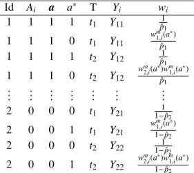
Table 1: Schematic display of the weighting in longitudinal mediation analysis Id Ai a a∗ T Yi wi 1 1 1 1 t1 Y11 pˆ1 1 1 1 1 0 t1 Y11 wm1,i(a∗) ˆ p1 1 1 1 1 t2 Y12 pˆ11 1 1 1 0 t2 Y12 w m 2,i(a ∗ )wm 1,i(a ∗ ) ˆ p1 ... ... ... ... ... ... ... 2 0 0 0 t1 Y21 1−1pˆ 2 2 0 0 1 t1 Y21 w m 1,i(a ∗ ) 1−pˆ2 2 0 0 0 t2 Y22 1−1pˆ2 2 0 0 1 t2 Y22 w m 2,i(a ∗)wm 1,i(a ∗) 1−pˆ2
The mediator weight (Appendix 1) for theithindividual at timetcorresponding to counterfactual
YtaM ta∗ is then wmt,i(a∗)= t Y s=1 P(Mt =ms,i|A=a∗,Ls=ls,i,Ms−1=ms−1,i) P(Mt =ms,i|A=a,Ls=ls,i,Ms−1=ms−1,i) . (11)
The validity of this approach follows from references (5) and (9). While reference (5) focuses on interventional analogues to direct and indirect effect, it provides identical identification results as in (9), rendering the inverse weighting strategy in (5) applicable. Note that (5) does not consider estimation of natural effect models, however.
3.2.3 Fitting the natural effect models
For binary exposure (coded 0 or 1), the general process for estimating the natural effect models can be described as follows:
1. Fit a suitable model for the exposure (e.g. equation 8) on the original data.
2. For each timet= 1, ...,T, fit a suitable model for the mediator (e.g. if Mt is categorical, one may use equation 10) conditional on the history of previous mediators, exposures and time-varying confounders, where the latter may include the outcome history. This can also be based on one model across all times fitted using pooled regression.
3. Construct a new data set by replicating each observation in the original data set twice for each time point and include an additional variable a∗, wherea∗is equal to the original exposure (A) for the first replication and equal to 1− Afor the second replication. In addition add an identification variable to indicate which data rows originate from the same subject, along with a visit time indicator,t=1,2, ...,T (see Table 1).
4. At timetthe weight for theithindividual corresponding to entrya∗ = 0,1 in Table 1 is computed as
wt,i(a∗)=wiawmt,i(a∗).
5. Fit the natural effect models (equation 7) by regressing the outcome on time t, a and
a∗ and the time interactions (ta,ta∗) on the basis of expanded data set, using weighted Generalised Estimating Equations (GEE) with independence working correlation. The weights in this regression are the weights (wt,i(a∗)) computed in the previous step. Note
A
L
0L
1M
1L
2...
L
T−1M
2...
M
TY
TU
Figure 2:Causal Directed Acyclic Graph with exposure induced mediator-outcome confounders. There can be unmeasured confounders between any selected time periods. However, to keep the DAG simple we display the unmeasured confounder at only one time point. The vectorsLtat timet=1, . . . ,(T−1)
includeYt.
that the use of an independence working correlation is critical to ensure that the right weights are assigned to the right records (17).
The above procedure can easily be implemented in standard software (Appendix 2). When the natural effect models include baseline covariates, e.g.g{E[Yt,a,M
t,a∗|L0]}=α0+α1a+α2a ∗+α
3t+ α4L0+α5t.a+α6t.a∗+α7a.L0+α8a∗.L0, thenwai can be set to 1 for all individuals because the
adjustment for confounding byL0now happens via a standard regression adjustment (10, 11). The resulting weights,wt,i(a∗) will typically be more stable (10, 11).
4
Estimation of standard errors and confidence intervals
To compute confidence intervals for the parameters indexing a natural effect models, it is tempt-ing to rely on the standard GEE output. However, unlike with weighttempt-ing procedures for marginal structural models, this does not guarantee conservative intervals. The bootstrap forms an attrac-tive alternaattrac-tive, but may have the drawback that when the mediators are categorical, some of the categories might not be selected in every bootstrap replication. It is for this reason we give an alternative method for computing the variance (18), which forms a hybrid between the use of robust standard error estimators from the GEE output, and the parametric bootstrap. The pro-posed procedure for computing the correct confidence intervals and standard error is described as follows:
Step-1 Fit a model for the exposure (e.g. logistic ifAis binary) and extract the regression
coeffi-cients and their covariance matrix.
Step-2 Fit a model for the mediator (e.g multinomial ifMis categorical), for each time point as described in the above section, and extract the regression coefficients and their covariance
matrix.
Repeat the following procedureB(e.g. B=1000) times:
Step-3 Randomly perturb the estimated coefficients from steps 1 and 2 by adding mean zero normal noise with covariance matrix as estimated in steps 1 and 2.
Step-4 Using the sampled coefficients from step 3, recompute the weights as described in equa-tion 11.
Step-5 Using these new set of weights, estimate the coefficients corresponding toa,a∗,ta, and
ta∗in the natural effect models.
Step-6 In the jth iteration, for j = 1, ...,B, store the regression coefficients, ˆα(j), and their variance-covariance,Var( ˆα|wˆj), from step 5. Here, the notationVar( ˆα|wˆj) expresses the
uncertainty at fixed weights.
Step-7 Using the results from theseBiterations estimate the variance-covariance of the regression coefficients corresponding toa,a∗,ta, andta∗using the formula
1 B B X j=1 Var( ˆα|wˆj)+ 1 B−1 B X j=1 ˆ α(j)−B−1 B X k=1 ˆ α(k) ˆ α(j)−B−1 B X k=1 ˆ α(k) 0 .
Step-8 A confidence interval for thekthcomponent ofαcan be obtained as ˆαk±1.96×sek, where
the standard error sek is the square root of the element in thekthrow andkthcolumn of
the matrix computed in step 7.
5
Illustrating Example
As an illustrating example we use the data from the Millennium Cohort Study (MCS), a lon-gitudinal study of children born in the UK between September 2000 and January 2002, which has been described elsewhere (19). Ethical approval for the MCS was received from a Research Ethics Committee at each time point of the survey round. Data were obtained from the UK Data Archive, University of Essex in March 2014. The first study contact with the cohort child was at 9 months, with survey interviews carried out by trained interviewers in the home with the main respondent (usually the mother) and their partner. Information was collected on 72% of those approached, providing information on 18,818 infants. For the analysis, data was used from four waves, when the children were aged 3, 5, 7 and 11 years. The total number of respondents who had participated in all four waves (by the age of 11 years of child) had declined to 10,313 (56% of the respondents who had taken part at the 9 months time period). To illustrate the techniques developed in this paper we use complete cases, N = 5188. Basic descriptives for some of the variables considered (e.g. Strengths and Difficulty Questionnaire at 3, 5, 7 and 11) show that the distribution of “Yes” categories in complete cases are slightly under-represented compared to the distributions of “Yes” in observed cases (20); similar is the observation for the maternal psychological distress variable. Further, for baseline confounders such as maternal education, missing cases were primarily from lower education categories such as “O-Levels/GCSE” and “Others”.
In our illustration, we are interested in examining the extent to which socio-economic position (SEP) in infancy and maternal psychological distress measured over the period of child devel-opment (ages 3 5 7 and 11 years) affect child mental health measured at the age of 11 years. The baseline confounders considered for SEP-child mental health relation were maternal education
Table 2: Schematic display of the weighting for the end of study outcome Id Ai a a∗ Yi wi 1 1 1 1 Y14 p1ˆ 1 1 1 1 0 Y14 wi(a∗) 2 0 0 0 Y24 1−1pˆ2 2 0 0 1 Y24 wi(a∗) ... ... ... ... ... ...
(L01), ethnicity (L02), gender (L03), marital status (L04) and age of mother (L05). Even though this is not a very comprehensive list of baseline confounders, we believe it to be a predominant subset of confounders of the relation between SEP and child mental health. The exposure (SEP) was categorised as “Above 60% median” and “below 60% median”. Maternal psychological distress was measured using the Kessler-6 scale, a self-reported measure collected from the mother of the child by asking how often in the past 30 days she had felt: “So depressed that nothing could cheer you up”, “Hopeless”, “Restless or Fidgety”, “That everything was an ef-fort”, “Worthless” and “Nervous”. Each of these items had a five-point response from “None of the time” (0) to “All of the time” (4). Responses to each item were combined to produce a single score ranging from 0 to 24. Scores exceeding 8 were truncated at 8. Child mental health problems were assessed using the Strengths and Difficulties Questionnaire, a 25-item measure completed by the mother. The overall score was classified into two groups “Normal”, 0, if the child had a score in between 0 and 13 and “Border-line abnormal”, 1, if they had score in between 14 and 40. These cut-offs were chosen based on recommended guidelines (21). In this illustration we present two scenarios where we take the outcome measured at the end of study, and the outcome measured from each time period. First, we estimate the effect of the parental SEP when the child’s age was 9 months, on the child’s mental health at age 11, with the mediators being maternal psychological distress measured at birth. The time-varying confounders include the time-varying outcomes and mediators measured at ages 3, 5 and 7, which we believe to be the main confounders, although we acknowledge that there may be other confounding factors such as family environment, medical treatment and others, which were unavailable. We then fitted a logistic natural effect models without the interaction term between exposure and mediator (P=0.968). The indirect effectβ2 in this model captures the combined effect along all pathways wherebyAdirectly affects one of the mediators, which may
then subsequently affect outcome at age 11. The direct effectβ1 captures the combined effect along all remaining pathways.
To estimate the direct and indirect effect on the end of study outcome, the data needs to be arranged as shown in Table 2. Results from this analysis show that SEP in childhood has a bigger effect compared to the effect via maternal psychological distress. The effect through SEP is 0.544 (corresponding to an odds ratio of exp(0.544)=1.72, 95% confidence interval (CI) 1.27 to 2.33). The effect via maternal distress is 0.122 (corresponding to an odds ratio of exp(0.122)=1.13, 95% CI 1.07 to 1.20), thus indicating that most of the effect is not via maternal distress.
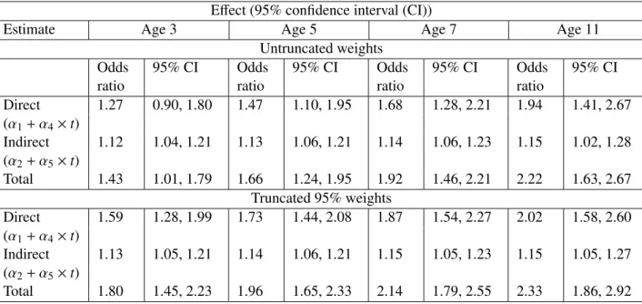
We next estimated the direct and indirect effect on all outcomes. For this purpose, the data needs to be arranged as in Table 1. Using logistic regression for the binary outcome, we estimated the time-specific effects. The distribution of weights for each time point is given in Figure 3. The estimates of the time/path specific effects are presented in Table 3. From Table 3 we note that both the maternal mental health and SEP contributed to the well-being of a child. Table 3 provides the odds ratios from the fitted natural effect model. For instance, for an individual
Figure 3: Distribution of exposure weights (upper left panel), mediator weights (upper right panel), untruncated weights (lower left panel) and the final 95% truncated weights (lower right panel).
Table 3: Odds ratio estimates from longitudinal mediation analysis using natural effect models Effect (95% confidence interval (CI))
Estimate Age 3 Age 5 Age 7 Age 11
Untruncated weights Odds ratio 95% CI Odds ratio 95% CI Odds ratio 95% CI Odds ratio 95% CI Direct 1.27 0.90, 1.80 1.47 1.10, 1.95 1.68 1.28, 2.21 1.94 1.41, 2.67 (α1+α4×t) Indirect 1.12 1.04, 1.21 1.13 1.06, 1.21 1.14 1.06, 1.23 1.15 1.02, 1.28 (α2+α5×t) Total 1.43 1.01, 1.79 1.66 1.24, 1.95 1.92 1.46, 2.21 2.22 1.63, 2.67 Truncated 95% weights Direct 1.59 1.28, 1.99 1.73 1.44, 2.08 1.87 1.54, 2.27 2.02 1.58, 2.60 (α1+α4×t) Indirect 1.13 1.05, 1.21 1.14 1.06, 1.21 1.15 1.05, 1.23 1.15 1.05, 1.27 (α2+α5×t) Total 1.80 1.45, 2.23 1.96 1.65, 2.33 2.14 1.79, 2.55 2.33 1.86, 2.92
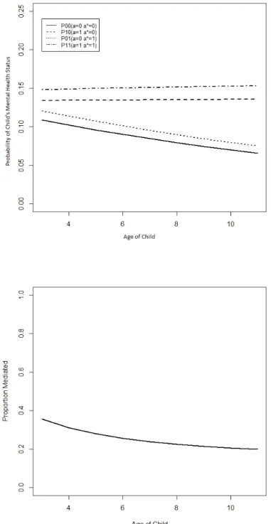
child, altering the level of socio-economic position from high (=0) to low (=1), while controlling the maternal psychological distress at the levels as naturally observed at any given level of SEP, a, almost doubles (exp(α1 + α4 ∗3 = 0.662) = 1.94; 95 % CI 1.41, 2.67) the odds of displaying mental health issues at age 11. This is much more pronounced than at age 3 (exp(α1+α4∗0 = 0.241) = 1.27; 95 % CI 0.90, 1.80). This may be partly explained by the fact that the mental health at age 3 was reported by parents and not the children themselves. Similarly, altering levels of maternal psychological distress as observed at low SEP to levels that would have been observed at high maternal distress while controlling their SEP at any given level, a, increases the odds of a child suffering from mental health issues at age 11 (exp(α2 + α5∗3 = 0.135) = 1.14; 95% CI: 1.02, 1.28). Similar results were obtained using truncated weights. The truncated weights were computed by resetting the value of weights greater than 95thpercentile (weight=6.1) to the value of the 95thpercentile (6.1). Figure 4 shows the trend in the direct and indirect effect over the period. It can be seen that the total effect (SEP and history of maternal psychological distress) increases over the period. In addition, the direct effect of SEP on child mental health was observed to have long term effects. On the other hand, the effect via maternal psychological distress on child mental health was almost constant. To estimate the proportion mediated we first computed the probabilities, P00,P01,P10, and P11, where Pkl is the probability of boarder line abnormal child mental health whenais set tok = 0,1 anda∗is set tol= 0,1 calculated using equation 7 with logit link. For examplePa.a∗ was computed as = exp(α0+α1a+α2a∗+α3t+α4ta+α5ta∗)
1+exp(α0+α1a+α2a∗+α3t+α4ta+α5ta∗). Figure 5 (top panel) shows the plot of these probabilities and
the proportion mediated (P11−P10)
(P11−P00), using untruncated weights. From Figure 5 (bottom panel) we
note that the proportion mediated declines over time. Inference does not seem to change when using truncated weights (see Figure 4, right panel).
6
Discussion
We have generalised the popular class of marginal structural models, which parameterise the effect of a point exposure on a (possibly time-varying) outcome, to enable effect decomposition w.r.t. a time-varying mediator in the presence of time-varying confounding. We have focussed on the situation where the mediator was multinomial, although the proposed inverse weighting strategy for fitting these models is readily adapted to mediators of arbitrary type (e.g. binary, continuous, count). Caution is warranted, however, when working with continuous mediators, because the proposed approach then requires inverse weighting by the mediator density, which can easily lead to instability. While we have focussed on dichotomous exposures, the proposal is also readily extended to arbitrary exposure distributions. As in Vansteelandt et al.(11), this re-quires augmenting the observed data set by picking for example, five random valuesa∗from the exposure distribution and next following steps 2-6 described in the above section. To avoid in-verse weighting by the exposure density, one may then consider standard regression adjustment for confounding of the exposure-outcome association.
The validity of the proposed approach critically relies on the assumptions expressed by Figure 2. In particular, we assume that adjustment for the measured confoundersL0suffices to identify the effect of exposure on all mediators, time-varying confounders and outcome. We moreover assume that no unmeasured variables are simultaneously associated with the mediator on the one hand, and time-varying confounders or outcome on the other hand. We thus in particular assume that the effect of time-varying confounders at timeton future mediators is unconfounded after adjusting for the history of all available measurements prior to time t. More importantly, we assume that the effect of mediators at timeton future time-varying confounders and outcome is unconfounded after adjusting for the history of all available measurements prior to timet. These assumptions are strong and may be especially implausible when the available number of
time-Figure 4: Trend in direct, indirect and total effect of socio-economic position and maternal psy-chological distress on child mental health status, using untruncated (left) and truncated weights (right).
Figure 5: Graphical presentation of the probability of child’s mental health status (top) and proportion mediated using untruncated weights (bottom).
varying confounders is large, as it may then be difficult to believe that all of them are associated with future mediators only by means of a causal effect. Similar assumptions can for instance be avoided when the aim is to assess the overall effect of the time-varying mediators on outcome. Traditional approaches for longitudinal mediation analysis (e.g. MacKinnon, 2008 (22)) also necessitate such assumptions, although they may not explicate them; in fact, many approaches assume in addition that also the effect of time-varying confounders at timeton future outcomes is unconfounded after adjusting for the history of all available measurements prior to time t, which is especially difficult to believe when there is confounding by past outcomes.
Like other approaches for path-specific effects (1), the proposed approach additionally relies on so-called cross-world counterfactual independencies (23, 24). These can be viewed as a strengthening of the assumptions listed in the previous paragraph, in the following sense. For instance, with a single mediator and a dichotomous exposure, assumption (2) (together with assumption (1) and substituting a by a∗) implies that Ya∗m ⊥⊥ Ma∗|L0. This shows that the cross-world independence assumption (4) is closely related to the ignorability assumption (2). In particular, assumption (2) expresses that subjects who would have low versus high levels of the mediator if given exposurea∗ are exchangeable (within strata ofL0) in terms of what their outcome would be if given exposurea∗and if their mediator were set tom. Assumption (4) expresses that such individuals should additionally be exchangeable in terms of what their outcome would be if given exposure aand if their mediator were set to m. In our opinion, it is usually hard to imagine that investigators could have such detailed knowledge to understand that assumption (2) holds, but not (4). In particular, if the investigators judge subjects with low versus high levels of the mediator at a given exposurea∗to be exchangeable (within strata ofL0), then we would generally believe them to be exchangeable in terms of bothYa∗mandYam. In that sense, we personally view the additional cross-world counterfactual independencies as relatively more innocent. Even so, the need for cross-world counterfactual independence assumptions is frustrating, as it implies that the aforementioned exchangeability cannot be avoided, even if data were available from multiple randomised experiments which randomised either exposure or mediators (or confounders), as it is needed to tie together the effects over the different paths. Despite this, by interpreting the obtained (in)direct effect as interventional (in)direct effect (7, 5), one can avoid the need for cross-world independence assumptions, along with the assumption that the effect of time-varying confounders at timeton future mediators is unconfounded after adjusting for the history of all available measurements prior to time t. Interventional direct effect express the effect of changing the exposure while fixing the repeated mediators at random draws from their conditional distributions at each time, given the history of the measurements observed until that time (while fixing the exposure at a given level, the previous mediators at the previously drawn values, and the previous time-dependent confounders at the levels that would naturally arise under such intervention). These effects differ from the interventional effects in (4, 25) who consider random draws from the distribution of the mediator at a certain exposure level conditional only on baseline covariates. By conditioning only on baseline covariates, these draws are less representative for what that an individual might have “naturally” experienced, making these estimands arguably less suitable to develop insight into mechanism (9).
In summary, we have described a simple, generic procedure for estimating direct and indirect effect of an exposure on an outcome in a longitudinal setting. The procedure can be applied in standard software (see Appendix 2 for an R implementation). As with all inverse weighting methods, monitoring of the distribution of the inverse probability weights is recommended to detect possible instabilities. In future work, we will extend the proposal to time-varying expo-sures, as well as examine the possibility of using fitting strategies for the inverse probability weights aimed at preventing instabilities.
Acknowledgement
MNM and SV equally contributed to both development and writing of this manuscript. MNM was funded by the Endeavour Executive scholarship from the Department of Education, Aus-tralia, to carry out the work presented. We would like to thank Dr. Steven Hope from the Insti-tute of Child Health, University College London, London, UK for sharing the UK Millennium Cohort data. The authors would like to declare no conflict of interest.
References
[1] Avin C, Shpitser I, Pearl J. Identifiability of path-specific effects. IJCAI-05. In: Proceed-ings of the Nineteenth International Joint Conference on Artificial Intelligence; 2005. p. 357–363.
[2] VanderWeele TJ, Vansteelandt S, Robins JM. Effect Decomposition in the Presence of an Exposure-Induced Mediator-Outcome Confounder. Epidemiology. 2014;2:300–306. [3] Bind MAC, Vanderweele TJ, Coull BA, Schwartz JD. Causal mediation analysis for
lon-gitudinal data with exogenous exposure. Biostatistics. 2016;17(1):122. Available from: +http://dx.doi.org/10.1093/biostatistics/kxv029.
[4] VanderWeele TJ, Tchetgen Tchetgen EJ. Mediation analysis with time varying exposures and mediators. Journal of the Royal Statistical Society: Series B (Statistical Methodology). 2017;79(3):917–938.
[5] Zheng W, van der Laan MJ. Mediation Analysis with Time-Varying Mediators and Expo-sures. In: Targeted Learning in Data Science. Springer; 2018. p. 277–299.
[6] Steen J, Loeys T, Moerkerke B, Vansteelandt S. medflex: An R Package for Flexi-ble Mediation Analysis using Natural Effect Models. Journal of Statistical Software. 2017;76(11):1–46.
[7] Vansteelandt S, Daniel RM. Interventional effects for mediation analysis with multiple mediators. Epidemiology. 2016;.
[8] Ilya S. Counterfactual Graphical Models for Longitudinal Mediation Analysis With Un-observed Confounding. Cognitive Science. 2013;37(6):1011–1035.
[9] Vansteelandt S, Linder M, Vandenberghe S, Steen J, Madsen J. Mediation analysis of time-to-event endpoints accounting for repeatedly measured mediators subject to time-varying confounding. Statistics in Medicine. 2019;in print.
[10] Lange T, Vansteelandt S, Bekaert M. A Simple Unified Approach for Estimating Natural Direct and Indirect Effects. American Journal of Epidemiology. 2012;176(3):190–195. Available from: http://aje.oxfordjournals.org/content/176/3/190.long. [11] Vansteelandt S, Bekaert M, Lange T. Imputation strategies for the estimation of natural
direct and indirect effects. Epidemiologic Methods. 2012;1(1):131–158.
[12] VanderWeele TJ. Explanation in causal inference: methods for mediation and interaction. Oxford University Press; 2015.
[13] Pearl J. Causality: Models, Reasoning, and Inference. New York: Cambridge University Press; 2000.
[14] VanderWeele TJ, Vansteelandt S. Conceptual issues concerning mediation, interventions and composition. Statistics and its Interface. 2009;2(4):457–468.
[15] Robins JM, Greenland S. Identifiability and Exchangeability for Direct and Indirect Ef-fects. Epidemiology. 1992 mar;3(2):143–155.
[16] Daniel RM, De Stavola BL, Cousens SN, Vansteelandt S. Causal mediation analysis with multiple mediators. Biometrics;71(1):1–14.
[17] Vansteelandt S. On Confounding, Prediction and Efficiency in the Analysis of Longitudinal and Crosssectional Clustered Data. Scandinavian Journal of Statistics;34(3):478–498. [18] Davison AC, Hinkley DV, Young GA. Recent developments in bootstrap methodology.
Statistical Science. 2003;p. 141–157.
[19] Connelly R, Platt L. Cohort profile: UK millennium Cohort study (MCS). International journal of epidemiology. 2014;43(6):1719–1725.
[20] Hope S, Pearce A, Chittleborough C, Deighton J, Maika A, Micali N, et al. Temporal effects of maternal psychological distress on child mental health problems at ages 3, 5, 7 and 11: analysis from the UK Millennium Cohort Study. Psychological Medicine. 2018;p. 111.
[21] Goodman R. The Strengths and Difficulties Questionnaire: A Research Note. Journal of Child Psychology and Psychiatry. 1997;38(5):581–586.
[22] MacKinnon DP. Introduction to statistical mediation analysis. Routledge; 2008.
[23] Robins JM, Richardson TS. Alternative graphical causal models and the identification of direct effects. In: Shrout P, editor. Causality and Psychopathology: Finding the Determi-nants of Disorders and Their Cures. Oxford, England: Oxford University Press; 2010. p. 103–158.
[24] Naimi AI. Invited Commentary: Boundless SciencePutting Natural Direct and In-direct Effects in a Clearer Empirical Context. American Journal of Epidemiology. 2015;182(2):109–114.
[25] Lin S, Young JG, Logan R, VanderWeele TJ. Mediation analysis for a survival out-come with time-varying exposures, mediators, and confounders. Statistics in medicine. 2017;36(26):4153–4166.
There are three parts to this appendix 1) Detailed derivations of the weight procedure described in main text of the paper 2) R-code to conduct both the analysis using the proposed method and code for computing the variance using the proposed method in section 4 of the main paper and 3) Derivation of the variance method, code to generate data and conduct simulations to compare the performance of the perturbed bootstrap method.
Appendix 1
This appendix presents detailed derivations of the procedure described in the main text. The derivation is closely related to the theorems in Lange et.al (10), but here we extended to longi-tudinal mediators for estimating natural direct and indirect effects.
We assume that the causal diagram of Figure 2 holds and represents a non-parametric structural equation model with independent errors (13). It then follows from Vansteelandt (9) that we can linkE[Yt(a,M
t,a∗)] to the observed data as:
E[Yt(a,M t,a∗)] = X mT X lT E[Y|A=a,MT =mT,LT =lT] T Y t=1 P[Mt=mt|A=a∗,Mt−1=mt−1,Lt=lt] ×P[Lt=lt|A=a,Mt−1=mt−1,Lt−1=lt−1] o P(L0=l0) =X a X mT X lT E[Y|A=a,MT =mT,LT =lT]{I(A=a)/P(A=a|L0=l0)}P(A=a|L0=l0) × T Y t=1 P[Mt=mt|A=a∗,Mt−1=mt−1,Lt=lt]P[Lt=lt|A=a,Mt−1 =mt−1,Lt−1 =lt−1] P(L0=l0) =X a X mT X lT E[Y|A=a,MT =mT,LT =lT]{I(A=a)/P(A=a|L0=l0)}P(A=a|L0=l0) × T Y t=1 P[Mt=mt|A=a,Mt−1=mt−1,Lt=lt]P[Lt=lt|A=a,Mt−1=mt−1,Lt−1=lt−1] P(L0=l0) × T Y t=1 P[Mt=mt|A=a∗,Mt−1=mt−1,Lt=lt] P[Mt=mt|A=a,Mt−1=mt−1,Lt=lt] P(L0=l0) =E[Y I(A=a)W]
where we defineM0to be empty and whereWrefers to the product of the weightsWiaWtm,i(a∗). This mo-tivates the proposed weighting procedure. For the estimators to have good performance infinite weights must be avoided. Our proposal therefore relies on the positivity assumption thatP(mt|A=a,Mt−1,Lt)>
σ >0 with probability 1 for allt,mt,aandP(A=a|L0)> >0 with probability 1 for alla.
Appendix 2
Data structure
Initially we load the original data set into variable named ‘mydata’, with observed exposure (A), outcome (Y1,Y2,Y3,Y4), mediator measured at four time points (M1,M2,M3andM4) and the confounders (L0). Next we construct new variables id, and ‘Astar’ where the latter corresponds to the value of the exposure relative to the indirect path. We also replicate a new data set by replicating the original two times such that ‘Astar’ takes the two different possible values through the replications. We repeat this process for each mediator.
First read the data into a matrix/dataframe/vector named mydata mydata<-read.csv(file="mentalhealth.csv",header=TRUE,sep=",")
N<-nrow(mydata)
#creating an Id variable mydata$id<-1:N
#L0 has five variables hence L01 L02 L03 L04 L05. # M1 M2 M3 M4 mediator observed at times 0 1 2 and 3. head(mydata, n=10L)
Data could not be provided due to confidentiality issues. #We have mediator measured at four time points.
#To implement the method described in the paper #we duplicate the data set twice for each mediator, mydata1<-mydata
mydata2<-mydata
mydata1$Astar<-mydata$A mydata2$Astar<-1-mydata$A
#thus creating 8 (4x2) replicates of original data, #we name this duplicated data as newmydata;
newmydata<-rbind(mydata1,mydata2,mydata3,mydata4,mydata5,mydata6,mydata7,mydata8) #data will now look like
> head(newmydata,n=16) #Data set names
#A: Exposure; Y: Outcome Astar: Duplicated exposure #Id: Respondent ID; W: Weights untruncated;
#W95: Weights truncated at 95%Percentile. newmydata[1097:1112,]
Data could not be published due to confidentiality reasons #95th percentile are truncated.
#Exposure weights before truncation > summary(newmydata[,"W"])
Min. 1st Qu. Median Mean 3rd Qu. Max. 0.3 1.0 1.1 2.0 1.5 53.6 #Exposure weights after truncation
> summary(newmydata[,"W95"])
Min. 1st Qu. Median Mean 3rd Qu. Max. 0.31 1.03 1.12 1.75 1.46 22.17
R-code for binary exposure, multinomial mediator and binary outcome
This example is similar to that described in main document. Here we use socio-economic position as the exposure (denotedA), measured at 9 months of (child) age, the mediator maternal psychological distress (denoted byM1,M2,M3,andM4), measured at ages 3, 5, 7 and 11, and the outcome, child development (denoted Y), measured at age 11. The considered confounders of the exposure-outcome relation are maternal education, ethnicity and marital status as a proxy for family environment. The time-varying confounders include the number of siblings, the previous outcomes and mediators measured at ages 3, 5 and 7.
Step-1:We first load the data set (e.g. mental health data) into a vector named “mydata” in R. Then fit a generalised linear regression to the mediator (mental psychological distress) at each of the four time points separately, conditioning on the exposureAand the confounders listed above (which include the history of outcomes and mediators at each time). Since the mediator is a categorical variable we used the vector generalised linear model (vglm), with family being multinomial, from the VGAM library in
R. m1creg <- vglm(M1˜A+factor(L01)+factor(L02)+factor(L03)+factor(L04)+factor(L05) ,data=mydata,family=multinomial) m2creg <- vglm(M2˜factor(M1)+A+Y1+factor(L01)+factor(L02)+factor(L03) +factor(L04)+factor(L05),data=mydata,family=multinomial) m3creg <- vglm(M3˜factor(M2)+factor(M1)+Y2+Y1+A+factor(L01)+factor(L02) +factor(L03)+factor(L04)+factor(L05),data=mydata,family=multinomial) m4creg <- vglm(M4˜factor(M3)+factor(M2)+factor(M1)+Y2+Y1+Y3+A+factor(L01) +factor(L02)+factor(L03)+factor(L04)+factor(L05), data=mydata,family=multinomial)
Step-2:In this step we create a new data set by replicating the original two times. Next we create a new variableId, which is a subject identifier, andAstarwhich takes once takes the value contained inAfor each subject, and once the opposite value1-A.
N <- nrow(mydata) mydata$id <- 1:N mydata1 <- mydata mydata2 <- mydata mydata1$Astar <- mydata$A mydata2$Astar <- 1-mydata$A newmydata <- rbind(mydata1,mydata2)
Step-3:The weights are computed from the predicted probabilities of the above multinomial regressions. For the numerator computation in weight equation 11 we used 1−Aand for the denominator we use used
Aas explanatory variables: #denominator weights m1pdr <- as.matrix(predict(m1reg,type="response",newdata=mydata)) [cbind(1:nrow(mydata),mydata$M1)] m2pdr <- as.matrix(predict(m2reg,type="response",newdata=mydata)) [cbind(1:nrow(mydata),mydata$M2)] m3pdr <- as.matrix(predict(m3reg,type="response",newdata=mydata)) [cbind(1:nrow(mydata),mydata$M3)] m4pdr <- as.matrix(predict(m4reg,type="response",newdata=mydata)) [cbind(1:nrow(mydata),mydata$M4)] #numerator weights Dattemp <- mydata Dattemp$A <- 1 - Dattemp$A m1pnr<-as.matrix(predict(m1reg,type="response",newdata=Dattemp)) [cbind(1:nrow(mydata),mydata$M1)] m2pnr<-as.matrix(predict(m2reg,type="response",newdata=Dattemp)) [cbind(1:nrow(mydata),mydata$M2)] m3pnr<-as.matrix(predict(m3reg,type="response",newdata=Dattemp)) [cbind(1:nrow(mydata),mydata$M3)] m4pnr<-as.matrix(predict(m4reg,type="response",newdata=Dattemp)) [cbind(1:nrow(mydata),mydata$M4)]
The predict function produces a matrix with probabilities for all 9 possible values of the mediator. By including the argument[cbind(1 :nrow(mydata),mydata$M1)] we select the probabilities corresponding to the values actually observed for the mediator. This trick requires that the levels of the mediators start from 1 in the data set. Since in our data set the mediator values start from 0 we changed the original values of mediatorsmydata$M <−mydata$M+1, so that the above command(cbind(1 :nrow(mydata)) works.
Step-4: The weights for the exposure were created using the logistic regression conditioned on the baseline confounders.
Aregdr <- glm(A˜factor(L01)+factor(L02)+factor(L03)+factor(L04)+factor(L05) ,data=mydata,family=binomial)
ap <- predict(Areg,type="response")
wa <- ifelse(mydata$A==1,1/ap,1/(1-ap)) #weight of A.
Step-5:Finally the logistic natural effects model for the dichotomous outcome can be fitted. To obtain sandwich standard errors that account for the repeated measures nature of the data, we use thegeeglm function from the packagegeepackusing theIdvariable to indicate dependence. Note that thegeeglm function requires that the observations be sorted by theIdvariable.
library(geepack} newmydata <- newmydata[order(newmydata$id),] fit_out <- geeglm(Y˜A+Astar+t+I(t*A)+I(T*Astar),data=newmydata,corstr="independence", family="binomial", weights=W,id=newmydata$id,scale.fix=T) > summary(fit_out) Call:
geeglm(formula = Y ˜ A + Astar + T + I(T * A) + I(T * Astar),
family = "binomial", data = gdat, weights = W, id = newmydata$id, corstr = "independence", scale.fix = T)
Coefficients:
Estimate Std.err Wald Pr(>|W|) (Intercept) -2.10513 0.11583 330.28 < 2e-16 *** A 0.24105 0.16272 2.19 0.13851 Astar 0.11682 0.01725 45.87 1.3e-11 *** T -0.13763 0.03981 11.95 0.00055 *** I(T * A) 0.14047 0.06084 5.33 0.02097 * I(T * Astar) 0.00609 0.01133 0.29 0.59085 ---Signif. codes: 0 *** 0.001 ** 0.01 * 0.05 . 0.1 1 Scale is fixed.
Correlation: Structure = independence
Number of clusters: 5189 Maximum cluster size: 8
Code for computing the variance
The below code is for computing thevarianceusing the method described in section-4 of the manuscript.
Code for drawing samples
This section has three components; 1) adding error to coefficients of exposure regression, 2) adding error to the coefficients of mediator regression and 3) computing probabilities of the multinomial regression #Part-1: generating new set of weights for the exposure regression
library(mvtnorm) awts<-function(regfit){ sreg<-summary(regfit) cv<-sreg$cov.unscaled mdl<-model.matrix(regfit) cf<-sreg$coefficients[,1] l<-length(cf) pe<-rmvnorm(1,rep(0,l),cv) ncf<-cf+pe
ncf<-t(ncf) nodds<-mdl%*%ncf
nweights<-exp(nodds)/(1+exp(nodds)) return(nweights)
}
#Part-2: generating the error to be added to coefficients for the mediator regression library(mvtnorm) mcoeffs<-function(mfit){ coeff<-coef(mfit,matrix=TRUE) cv<-vcov(mfit) l<-dim(coeff)[1] k<-dim(coeff)[2] m<-l*k
#Since the mfit has coefficients corresponding to every level of a multinomial mediator #information from the coeff and cv matrix above need to be extracted carefully
#it is for this reason we at first developed an index, s,
#this index s now allows to extract the correct set of coefficients and covariances #corresponding to a level of a mediator.
s<-seq(1,m,k) #s: 1 9 17 25 33 41 49 57 65 73 81 89 97 ncoeff<-matrix(0,k,l) cf<-coeff[,1] cv1<-as.matrix(cv[s,s]) me<-rmvnorm(1,rep(0,l),cv[s,s]) ncoeff[1,]<-coeff[,1]+me for(i in 1:(k-1)){ cf<-coeff[,i+1] cv1<-as.matrix(cv[s+i,s+i]) men<-rmvnorm(1,rep(0,l),cv1) ncoeff[i+1,]<-cf+men } ncoeff<-t(ncoeff) return(ncoeff) }
#Part-3 program for computing the predicted probabilities in case of multinomial mediator trial<-function(mdl,ncoef){ ro<-dim(mdl)[1] co<-dim(mdl)[2] k<-ncol(ncoef) n<-ro/k rsm<-matrix(0,n,k) fs<-seq(1,ro,k) ss<-seq(1,co,k) rsm[,1]<-mdl[fs,ss]%*%ncoef[,1] for(i in 1:(k-1)){ pv<-mdl[fs+i,ss+i]%*%ncoef[,(i+1)] rsm[,(i+1)]<-pv } rsm<-exp(rsm) rs<-rowSums(rsm) s<-matrix(0,n,k) for(i in 1:n){ s[i,]<-rsm[i,]/(1+rs[i]) } rss<-rowSums(s) s<-as.data.frame(s) s$V9<-1-rss
s<-as.matrix(s) return(s) }
Code for computing the variance
Once the weights are recomputed from each simulation using the above code then the outcome regression needs to be performed for each simulation. Outcome regression coefficients and thevariance-covariance matrix from each of this simulation are stored to compute the final variance estimate that accounts for varying weights. To do the variance computation using the stored estimates we used the following code. #Code for exposure regression before conducting simulations
Aregdr<-glm(Atemp˜factor(L01)+factor(L02)+factor(L03)
+factor(L04)+factor(L05),data=mydata,family=binomial) #code for mediator regression from each time point before simulations m1reg<-vglm(M1˜Atemp+factor(L01)+factor(L02) +factor(L03)+factor(L04)+factor(L05) ,data=mydata,family=multinomial) m2reg<-vglm(M2˜factor(M1)+Atemp+Y1+factor(L01) +factor(L02)+factor(L03)+factor(L04)+factor(L05) ,data=mydata,family=multinomial(),maxit=500) m3reg<-vglm(M3˜factor(M2)+factor(M1)+Y2+Y1+Atemp+factor(L01) +factor(L02)+factor(L03)+factor(L04) +factor(L05),data=mydata,family=multinomial()) m4reg<-vglm(M4˜factor(M3)+factor(M2)+factor(M1)+Y2+Y1+Y3+Atemp +factor(L01)+factor(L02)+factor(L03) +factor(L04)+factor(L05),data=mydata,family=multinomial()) mdl1<-model.matrix(m1reg) mdl2<-model.matrix(m2reg) mdl3<-model.matrix(m3reg) mdl4<-model.matrix(m4reg) mydata$Atemp<-1-mydata$A m1creg<-vglm(M1˜Atemp+factor(C1)+factor(L01)+factor(L02)+factor(L03) +factor(L04)+factor(L05),data=mydata,family=multinomial) m2creg<-vglm(M2˜factor(M1)+Atemp+Y1+factor(L01)+factor(L02)+factor(L03) +factor(L04)+factor(L05),data=mydata,family=multinomial(),maxit=500) m3creg<-vglm(M3˜factor(M2)+factor(M1)+Y2+Y1+Atemp+factor(L01)+factor(L02)+factor(L03) +factor(L04)+factor(L05),data=mydata,family=multinomial()) m4creg<-vglm(M4˜factor(M3)+factor(M2)+factor(M1)+Y2+Y1+Y3+Atemp+factor(L01) +factor(L02)+factor(L03)+factor(L04)+factor(L05) ,data=mydata,family=multinomial()) mdlc1<-model.matrix(m1creg) mdlc2<-model.matrix(m2creg) mdlc3<-model.matrix(m3creg) mdlc4<-model.matrix(m4creg) M<-500 t<-matrix(c(0,1,2,3),1,4)
#full code of simulations using above code for(i in 1:M){
apdr<-awts(Aregdr)
wa<-ifelse(mydata$A==1,1/apdr,(1-mydata$A)/(1-apdr)) #weight of A. wa_95<-ifelse(wa>=quantile(wa,.95),quantile(wa,.95),wa)
c2<-mcoeffs(m2reg) c3<-mcoeffs(m3reg) c4<-mcoeffs(m4reg) mt1nr<-trial(mdlc1,c1)[cbind(1:nrow(mydata),mydata$M1)] mt2nr<-trial(mdlc2,c2)[cbind(1:nrow(mydata),mydata$M2)] mt3nr<-trial(mdlc3,c3)[cbind(1:nrow(mydata),mydata$M3)] mt4nr<-trial(mdlc4,c4)[cbind(1:nrow(mydata),mydata$M4)] mt1dr<-trial(mdl1,c1)[cbind(1:nrow(mydata),mydata$M1)] mt2dr<-trial(mdl2,c2)[cbind(1:nrow(mydata),mydata$M2)] mt3dr<-trial(mdl3,c3)[cbind(1:nrow(mydata),mydata$M3)] mt4dr<-trial(mdl4,c4)[cbind(1:nrow(mydata),mydata$M4)] #creation of new weights
wM1<-mt1nr/mt1dr mydata$wM1<-wM1*wa wM2<-(mt2nr/mt2dr)*wM1 mydata$wM2<-wM2*wa wM3<-(mt3nr/mt3dr)*wM2 mydata$wM3<-wM3*wa wM4<-(mt4nr/mt4dr)*wM3 mydata$wM4<-wM4*wa #truncated weights wM1<-mt1nr/mt1dr mydata$wM1_95<-wM1*wa_95 wM2<-(mt2nr/mt2dr)*wM1 mydata$wM2_95<-wM2*wa_95 wM3<-(mt3nr/mt3dr)*wM2 mydata$wM3_95<-wM3*wa_95 wM4<-(mt4nr/mt4dr)*wM3 mydata$wM4_95<-wM4*wa_95
#creation of final data for analysis
gdat1<-cbind(A=mydata$A,Y=mydata$Y1,Astar=mydata$A,T=0, id=1:nrow(mydata),W=wa,W_95=wa_95) gdat2<-cbind(A=mydata$A,Y=mydata$Y1,Astar=1-mydata$A,T=0, id=1:nrow(mydata),W=mydata$wM1,W_95=mydata$wM1_95) gdat3<-cbind(A=mydata$A,Y=mydata$Y2,Astar=mydata$A,T=1, id=1:nrow(mydata),W=wa,W_95=wa_95) gdat4<-cbind(A=mydata$A,Y=mydata$Y2,Astar=1-mydata$A,T=1, id=1:nrow(mydata),W=mydata$wM2,W_95=mydata$wM2_95) gdat5<-cbind(A=mydata$A,Y=mydata$Y3,Astar=mydata$A,T=2, id=1:nrow(mydata),W=wa,W_95=wa_95) gdat6<-cbind(A=mydata$A,Y=mydata$Y3,Astar=1-mydata$A,T=2, id=1:nrow(mydata),W=mydata$wM3,W_95=mydata$wM3_95) gdat7<-cbind(A=mydata$A,Y=mydata$Y4,Astar=mydata$A,T=3, id=1:nrow(mydata),W=wa,W_95=wa_95) gdat8<-cbind(A=mydata$A,Y=mydata$Y4,Astar=1-mydata$A,T=3, id=1:nrow(mydata),W=mydata$wM4,W_95=mydata$wM4_95)
#combining the data newmydata<-as.data.frame(rbind(gdat1,gdat2,gdat3,gdat4 ,gdat5,gdat6,gdat7,gdat8)) newmydata<-newmydata[order(newmydata$id),] newmydata<-newmydata[order(newmydata$id),] library(geepack) fitsepb<-geeglm(Y˜A+Astar+T+I(T*A)+I(T*Astar),id=newmydata$id, corstr="independence",family="binomial", weight=W,data=newmydata,scale.fix=T)
#extracting coefficients and variance covariance from each simulation cf<-summary(fitsepb)$coefficients
cv<-vcov(fitsepb)
#DE matrix of direct effects #IDE matrix of indirect effects
$VC variance covariance terms required DE[i,]<-c(cf[2,1],cf[5,1]) IDE[i,]<-c(cf[3,1],cf[6,1]) VC[i,]<-c(cv[2,2],cv[3,3],cv[5,5],cv[6,6], cv[2,3],cv[2,5],cv[2,6],cv[3,5] ,cv[3,6],cv[5,6]) #truncated 95 fitsepb_95<-geeglm(Y˜A+Astar+T+I(T*A)+I(T*Astar),id=newmydata$id, corstr="independence",family="binomial", weight=W_95,data=newmydata,scale.fix=T) #extracting coefficients and variance covariance matrices cf<-summary(fitsepb_95)$coefficients
cv<-vcov(fitsepb_95)
#DE direct effect coefficients matrix corresponding to truncated data #IDE indirect effect matrix
#Variance covariances corresponding to truncated data model fit. DE_95[i,]<-c(cf[2,1],cf[5,1]) IDE_95[i,]<-c(cf[3,1],cf[6,1]) VC_95[i,]<-c(cv[2,2],cv[3,3],cv[5,5],cv[6,6] ,cv[2,3],cv[2,5],cv[2,6], cv[3,5],cv[3,6],cv[5,6]) }
#compute the final estimate of direct, indirect and total effect for each simulation. #data for these are from the changing weights
#DE: Stores the coefficients required for computing the direct effect estimates #IDE: Stores the coefficients required for computing the indirect effect estimates #TE: total Effects
#DE[,1]: Has the values corresponding to alpha_1 from simulations #DE[,2]: Has the coefficients corresponding to alpha_4
#IDE[,1]: Has the values corresponding to alpha_2 from simulations #IDE[,2]: Has the values corresponding to alpha_5
DE_final<-DE[,1]+matrix(DE[,2],M,1)%*%t IDE_final<-IDE[,1]+matrix(IDE[,2],M,1)%*%t TE_final<-DE_final+IDE_final
#Step-2
#data for these are from the variance and covariance extract #from each simulation with new weights
#VC: Variance covariance estimates stored from each simulation DEV<-VC[,1]+matrix(VC[,3],M,1)%*%(tˆ2)+matrix(VC[,6],M,1)%*%(2*t) IDEV<-VC[,2]+matrix(VC[,4],M,1)%*%(tˆ2)+matrix(VC[,9],M,1)%*%(2*t) TEV<-VC[,1]+VC[,2]+matrix(VC[,3],M,1)%*%(tˆ2)+matrix(VC[,6],M,1)%*%(2*t) +matrix(VC[,4],M,1)%*%(tˆ2)+matrix(VC[,9],M,1)%*%(2*t) +matrix(VC[,5],M,1)%*%(2*t)+matrix(VC[,7],M,1)%*%(2*t) +matrix(VC[,8],M,1)%*%(2*t)+matrix(VC[,10],M,1)%*%(2*tˆ2) #Step-3
#Computing the new variance of the direct, indirect, and total effects #that account for the weight changes
DEvar<-apply(DE_final,2,var)+apply(DEV,2,mean) IDEvar<-apply(IDE_final,2,var)+apply(IDEV,2,mean) TEvar<-apply(TE_final,2,var)+apply(TEV,2,mean)
#Step-4 computing the lower and upper bounds of confidence interval #which accounts for variance due to changing weights.
#In this step I am using the initial estimates computed from the observed data and #stored in a matrix labelled "final".
#DEL: Direct effect lower; DEU: Direct effect upper; IDEL: Indirect effect lower; #IDEU: Indirect effect upper
#TEL: Total effect lower; TEU: Total effect upper. DEL<-final[1,]-sqrt(DEvar)*1.96 DEU<-final[1,]+sqrt(DEvar)*1.96 IDEL<-final[2,]-sqrt(IDEvar)*1.96 IDEU<-final[2,]+sqrt(IDEvar)*1.96 TEL<-final[3,]-sqrt(TEvar)*1.96 TEU<-final[3,]+sqrt(TEvar)*1.96
#Combining all the estimates to be reported
finalest<-rbind(DEL,final[1,],DEU,IDEL,final[2,],IDEU,TEL,final[3,],TEU) #the above process is then repeated for the truncated estimates.
If one estimates the total effect using an MSM by settingA =a∗and use the default GEE Std.err, and
compare it to the Std.err obtained using above described method they should more or less agree.
Appendix 3
Variance estimation
Let ˆαbe the estimator of the coefficient αindexing the natural effect model and ˆw be the estimated weight. Then it follows by the law of iterated variance that
Var( ˆα)=E{Var( ˆα|wˆ)}+Var{E( ˆα|wˆ)}.
Writing ˆα=αˆ(O,wˆ) as a function of the observed dataOand the estimated weights ˆw, we have that
E( ˆα|wˆ)= Z ˆ α(O,wˆ)f(O|wˆ)dO= Z ˆ α(O,wˆ)nf(O)+op(1)odO,
whereop(1) is a term that converges to zero in probability. That f(O|wˆ)= f(O)+op(1) can be seen upon noting that ˆwconverges to a deterministic function ofOin probability. It follows thatE( ˆα|wˆ) equals the mean of ˆα(O,w) withwsubstituted by ˆw, up to anop(1) term. Likewise,Var( ˆα|wˆ) equals the variance of ˆα(O,w) withwsubstituted by ˆw, up to anop(1) term. The variance of ˆα(O,w) can be consistently
estimated using a sandwich estimator, considering the weightwas known. It follows thatE{Var( ˆα|wˆ)}
can be consistently estimated as
1 B B X j=1 Var( ˆα|wˆj).
Further, the meanE( ˆα|wˆ) can be consistently estimated as ˆα(O,wˆ). It follows thatVar{E( ˆα|wˆ)}can be consistently estimated as 1 B−1 B X j=1 αˆ (j)−B−1 B X k=1 ˆ α(k) αˆ (j)−B−1 B X k=1 ˆ α(k) 0 .
Simulations for standard error estimation
In this section we present the code for simulating the data that was used for conducting single mediation analysis using natural effect models. We also present the code that was used in estimating the standard errors. Simulations were performed on a sample of 1000 observations and with 1000 perturbed bootstrap estimates.
#program for checking the variance.
#I am generating the values of exposure, mediator, confounders and outcome as Binary n<-1000 set.seed(562) C1<-rnorm(n) C2<-rbinom(n,1,0.4) A<-rbinom(n,1,(exp(0.05+0.1*C1+0.2*C2)/(1+exp(0.05+0.1*C1+0.2*C2)))) M<-rbinom(n,1,(exp(0.05+0.1*A-0.1*C1-0.2*C2)/(1+exp(0.05+0.1*A-0.1*C1-0.2*C2)))) Y<-rbinom(n,1,(exp(0.05+0.1*A+0.1*M-0.1*C1-0.2*C2)/(1+exp(0.05+0.1*A+0.1*M-0.1*C1-0.2*C2))))
#storing of the data set
sdat<-as.data.frame(cbind(Y,M,A,C1,C2))
write.table(sdat,file="sdat.csv",sep=",",row.names=FALSE)
#Conducting natural effects model in single mediator case. Atemp<-A
sdat$Atemp<-A
#creation of Inverse probability treatement weights Aregdr<-glm(Atemp˜C1+C2,data=sdat,family=binomial) ap<-fitted.values(Aregdr,type="response")
wa<-ifelse(sdat$A==1,1/ap,1/(1-ap)) #weight of A. #Creation of weights of M for eachi time period
M1reg<-glm(M˜Atemp+C1+C2,data=sdat,family=binomial("logit")) sdat$Atemp<-sdat$A
tdr1<-predict.glm(M1reg,newdata=sdat,type="response") sdat$Atemp<-1-sdat$A
tnr1<-predict.glm(M1reg,newdata=sdat,type="response") #creation of mediator weights
W<-tnr1/tdr1
#Adding Weight of M to data set sdat$wM1<-(tnr1/tdr1)*wa
#expanding data
gdat1<-cbind(A=sdat$A,Y=sdat$Y,Astar=sdat$A,id=1:nrow(sdat),W=wa)
#combining the data
gdat<-as.data.frame(rbind(gdat1,gdat2)) gdat<-gdat[order(gdat$id),]
#conducting final estimation using the GEEGLM model. library(geepack) library(BSagri) fitsepb<-geeglm(Y˜A+Astar,id=gdat$id,corstr="independence", family="binomial",weight=W,data=gdat,scale.fix=T) exp(fitsepb$coefficients) de_model<-fitsepb$coefficients[,2] ide_model<-fitsepb$coefficients[,3] de_odds<-exp(de_model) ide_odds<-exp(ide_model) te<-de_model+ide_model te-odds<-exp(te) vcc<-vcov(fitsepb) te_v<-vcc[2,2]+vcc[3,3]+2*vcc[2,3] te_se<-sqrt(te_v)
#Perturb method of bootstrap. #program for the weight generation.
#generating new set of weights for the exposure without re-sampling the data awts<-function(regfit){ sreg<-summary(regfit) cv<-sreg$cov.unscaled mdl<-model.matrix(regfit) library(mvtnorm) cf<-sreg$coefficients[,1] l<-length(cf) pe<-rmvnorm(1,rep(0,l),cv) ncf<-cf+pe ncf<-t(ncf) nodds<-mdl%*%ncf nweights<-exp(nodds)/(1+exp(nodds)) return(nweights) }
#genrating the distributions of coefficients for the mediator data
#generating new set of weights for the exposure without re-sampling the data mwts<-function(regfit,Atemp){ sreg<-summary(regfit) cv<-sreg$cov.unscaled mdl<-as.data.frame(model.matrix(regfit)) mdl$Atemp<-Atemp mdl<-as.matrix(mdl) library(mvtnorm) cf<-sreg$coefficients[,1] l<-length(cf) pe<-rmvnorm(1,rep(0,l),cv) ncf<-cf+pe ncf<-t(ncf) nodds<-mdl%*%ncf nweights<-exp(nodds)/(1+exp(nodds)) return(nweights)
}
#using 1000 perturb samples M<-1000 Dat<-sdat DE<-matrix(0,M,1) IDE<-matrix(0,M,1) VC<-matrix(0,M,3) library(geepack) library(BSAgri) #Final estimates for(i in 1:M){ apdr<-awts(Aregdr) wa<-ifelse(Dat$A==1,1/apdr,1/(1-apdr)) #weight of A. Atemp<-Dat$A wdr<-mwts(M1reg,Atemp) Atemp<-1-Dat$A wnr<-mwts(M1reg,Atemp) wM1<-wnr/wdr Dat$wM1<-wM1*wa
#creation of final data for analysis
gdat1<-cbind(A=Dat$A,Y=Dat$Y,Astar=Dat$A,id=1:nrow(Dat),W=wa)
gdat2<-cbind(A=Dat$A,Y=Dat$Y,Astar=1-Dat$A,id=1:nrow(Dat),W=Dat$wM1) #combining the data
gdat<-as.data.frame(rbind(gdat1,gdat2)) gdat<-gdat[order(gdat$id),] fitsepb<-geeglm(Y˜A+Astar,id=gdat$id,corstr="independence", family="binomial",weight=W,data=gdat,scale.fix=T) cf<-summary(fitsepb)$coefficients cv<-vcov(fitsepb) DE[i,]<-c(cf[2,1]) IDE[i,]<-c(cf[3,1]) VC[i,]<-c(cv[2,2],cv[3,3],cv[2,3]) }
#computing the variance of DE using the perturb bootstrap va<-var(DE)
mvde<-mean(VC[,1]) tvde<-va+mvde
#computing the variance of IDE using the perturb bootstrap vide<-var(IDE)
mvide<-mean(VC[,2]) tvide<-vide+mvide exp(mean(DE)) exp(mean(IDE))
#computing the total effect and its variance. Te<-DE+IDE
exp(mean(Te))
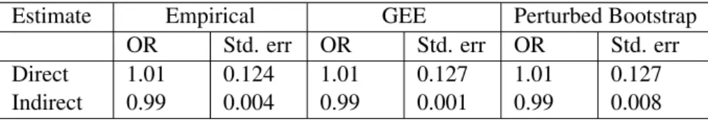
Table 4: Odds ratio (OR) estimates of direct and indirect effects estimated using simulated data. These estimates are computed using natural effect models. The standard error (Std. err) estimates are obtained using empirical estimates, generalized estimating equations (GEE) and perturbed bootstrap.
Estimate Empirical GEE Perturbed Bootstrap
OR Std. err OR Std. err OR Std. err
Direct 1.01 0.124 1.01 0.127 1.01 0.127
Indirect 0.99 0.004 0.99 0.001 0.99 0.008