A Classification Rules Mining Method based on
Dynamic Rules' Frequency
Issa Qabajeh
Centre for Computational Intelligence, De Montfort University, Leicester, UK
Francisco Chiclana
Centre for Computational Intelligence, De Montfort University, Leicester, UK
Fadi Thabtah Ebusiness Dept., CUD,
Dubai, UAE [email protected]
Abstract—Rule based classification or rule induction (RI) in data mining is an approach that normally generates classifiers containing simple yet effective rules. Most RI algorithms suffer from few drawbacks mainly related to rule pruning and rules sharing training data instances. In response to the above two issues, a new dynamic rule induction (DRI) method is proposed that utilises two thresholds to minimise the items search space. Whenever a rule is generated, DRI algorithm ensures that all candidate items' frequencies are updated to reflect the deletion of the rule’s training data instances. Therefore, the remaining candidate items waiting to be added to other rules have dynamic frequencies rather static. This enables DRI to generate not only rules with 100% accuracy but rules with high accuracy as well. Experimental tests using a number of UCI data sets have been conducted using a number of RI algorithms. The results clearly show competitive performance in regards to classification accuracy and classifier size of DRI when compared to other RI algorithms.
Keywords—Classification Rules, Data Mining, Rule Induction, Dynamic, Experimental tests.
1. INTRODUCTION
One of the popular tasks in data mining which involves predicting unseen target attribute (the class) based on learning from labelled historical data (training data set) is classification. The main goal of any classification technique is to accurately estimate the value of the class of an unseen data normally called the test data (Thabtah et al., 2015). This type of learning that occurred on the training data set is restricted to the value of the class attribute and therefore it falls under the category of supervised learning research area. Common applications of classification are medical diagnoses (RameshKumar et al., 2013), phishing detection (Abdelhamid et al., 2014), fraud detection (Whitten and Frank, 2005), etc. Some of the main classification approaches developed in data mining include Decision Trees (DT) (Quinlan, 1993), Neural Network (NN) (Mohammad et al., 2013), Associative Classification (AC) (Thabtah, et al., 2004) (Thabtah, 2005), and Rule Induction (RI) (Cendrowska, 1987). The latter two approaches extract classifiers that contain human interpretable rules in the form “If-Then”, which explain their wide spread applicability. However, there are differences between AC and RI especially in the way rules are induced as well as pruned. This article focuses on RI based classification.
PRISM is an RI technique, developed in (Cendrowska, 1987) and slightly enhanced by others (Stahl and Bramer, 2008), that follows separate and conquer learning strategy in building the classifier (Witten and Frank, 2005). For each class, this algorithm builds a set of rules and then combines all rules to make the classifier. Normally for a certain class, this algorithm starts with an empty rule and keeps adding attribute
values to the rule’s body until this rule reaches a certain expected accuracy (Definition 8- Section 2.2). When this happens, PRISM generates the rule, removes all data connected with it from the training data set and continues building other rules in the same way until no more data associated with the current class can be found. At this point, PRISM moves to a new class and repeats the same steps described earlier until the training data set becomes empty. During the building of a rule, often the largest expected accuracy attribute is added to the rule.
This paper investigates shortcomings associated with RI algorithms, in particular PRISM. Specifically, we look into the following three main issues:
Reducing the search space by using an item’s frequency threshold that we call (freq).
Remove the items overlapping among the discarded training instances of the generated rules’ and other candidate rules waiting to be produced. Usually, there is an impact when removing training instances linked to a generated rule on the other candidate items that have appeared in the deleted instances.
Generating not only perfect rules (expected accuracy 100%) but also other high quality rules. We utilise here a pre-defined user threshold that we call rule’s strength (Rule_Strength) to separate between acceptable and not acceptable rules.
We believe that the end user can control the items appearing within the generated rules by using a minimum item’s threshold to separate between survived items (items having data representation above the threshold) and weak items (items having a data representation below the threshold). By deleting the weak items early and whenever a rule is derived, the search space and running time decreased and consequently computation costs is reduced. Moreover, the item's threshold is used every time a rule is produced. Normally, the original frequency of items that have been computed from the training data set are not fixed, rather survived items' frequency are updated, often reduced, whenever a rule is produced because of the deletion of rule’s instances from the training data set.
In response to the above raised issues, in this article a new dynamic learning method based on RI that we name Dynamic Rule Induction (DRI) is developed. It discovers rules one by one per class and primarily uses a minimum frequency threshold to limit the search space for rules by discarding any weak items. For each generated rule belonging to a specific class, DRI updates the strong items frequencies that appeared within the deleted training instances of the generated rule. This indeed gives a more realistic classifier with less numbers of perfect rules leading to a natural pruning of items during the
rule discovery phase. More details on the distinguishing features of the proposed algorithm are given in Section 4.3. Lastly, DRI limits the use of the default class rule by generating near perfect rules and storing them in a secondary classifier. Often these rules are ignored by PRISM algorithm since they do not hold 100% expected accuracy. These rules are used instead of the default class rule only when no primary rule is able to classify a test data.
The rest of the paper is structured as follows: Section 2 covers the above three raised issues, the classification problem and its main related definitions. Section 3 surveys common RI algorithms, while Section 4 discusses the proposed algorithm and its related phases. Section 5 is devoted to the data and the experimental results analysis and closing the paper conclusions are provided in Section 6.
2. THE PROBLEM AND RAISED ISSUES
In this section we first introduce the raised research issues that the paper tackles and the classification problem in the context of RI.
A. Raised Research Issues
Issue 1.One of the main problems associated with RI
approaches such as PRISM is the large dimensionality of the items search space. When constructing a rule for a particular class, PRISM has to evaluate the expected accuracy of all available items linked with that class in order to select the best one to be added to the rule’s body. This is computationally expensive when the training data has many attribute values and can be a burden especially when several unnecessary computations are made for items that have low data representation (weak items).
Issue 2.Another serious problem not previously reported in RI research happens when instances of a generated rule are discarded by PRISM from the training data set. This usually impacts other items frequency sharing these instances with that rule. For example, when a rule R1: IF x1 and y2 Then C1 is generated, let us assume that 6 data instances linked with rule R1 have been discarded. Now, all candidate items inside the 6 deleted training data instances other than items “x1” and “y2” are impacted because of this removal and their frequencies as well as expected accuracies should be updated to reflect the occurred changes. This means that some of these candidate items may no longer hold enough frequency and therefore should be pruned before building the next rule. Issue 3.One of the problems associated with PRISM is its excessive learning (overfitting) to derive perfect rules regardless of whether the produced rule has a sufficient data representation, which may lead to the generation of massive number of rules with low frequency despite being perfect in regards to expected accuracy.
Given an input training data set T, which has n distinct attributes A1, A2, … , An, one of which is called the class, which contains a list of values. The Cardinality of T is denoted by |T|. An attribute may be nominal or continuous. The ultimate aim is to build a classification model (classifier) from T, e.g.
C
:
A
l
, which estimates the value of the class of test data where A is a disjoint set of attribute values andl
is a class.The proposed algorithm depends on a predefined user threshold called freq. This threshold is utilised to differentiate between strong and non-strong ruleitems (weak ruleitems) based on their frequency in the training data set. Any ruleitem that survives (see below Def. 7) the freq threshold is known as a strong ruleitem, and when the strong ruleitem belongs to one attribute, we call it a strong 1- ruleitem. Hereunder are the main related terms definitions.
Definition 1: An item is an attribute (Ai) plus its value (ai)
denoted (Ai, ai).
Definition 2: A training instance in T is a row combining a list of items (Aj1, aj1), …, (Ajv, ajv), plus a class denoted by cj.
Definition 3: A ruleitem r has the format<body, c>, where body is a set of disjoint items and c is a class value.
Definition 4: The frequency threshold (freq) is a predefined threshold given by the end user.
Definition 5: The body frequency (body_Freq) of a ruleitem r in T is the number of instances in T that match r’s body.
Definition 6: The frequency of a ruleitem r in T (ruleitem_freq) is the number of instances in T that match r.
Definition 7: A ruleitem r passes the freq threshold if it’s |body_Freq|/ |T| ≥ freq. Such a ruleitem is said to be a strong ruleitem.
Definition 8: A ruleitem r expected accuracy is defined as |ruleitem_freq|/ |body_Freq|.
Definition 9: A rule in the classifier is represented as:
l
body
, where the left hand side (body) is a set of disjoint attribute values and the right hand side(l
)is a class value. Thus, the rules representation is: a1a2...anl13. LITERATURE REVIEW
PRISM is one of the known RI algorithms that derive rules in greedy manner by splitting the training data set into subsets with respects to class values. Then for each subset, the algorithm forms an empty rule, searches for the attribute value that has the highest expected accuracy, appends it into the rule body, and continues finding attribute values until the current candidate rule has 100% accuracy as per Eq.(1).
(P/|T|) (1)
where P = the # of training data examples that are similar to the added item and the empty rule’s class and |T| = the size of the training data.
Once this happens, the algorithm generates the rule and removes all of its positive instances (data in the subset belonging to the rule). The same process is repeated to produce the rest of the rules from the remaining uncovered data in the subset until the subset becomes empty or no rule with satisfactory expected accuracy can be derived. At that point the algorithm moves on to the next class subset and repeats the same process until all rules in all class data subsets are generated and merged to form the classifier. One notable problem about this classification approach is that the required effort to find the best attribute value to append into a rule at any stage of the learning phase is disproportionate for high dimensional training data sets. Moreover, there is no clear pruning mechanism in PRISM, which often results in very large number of rules each covering a low number of instances within the classifier.
The RIPPER algorithm (Cohen, 1995) was developed to decrease the classifier size in RI. This algorithm divides the training data set with respect to class labels, and then starting with the least frequent class set builds a rule by adding items (attribute values) to its body until the rule is perfect (the number of negative examples covered by the rule is zero). For each candidate empty rule, the algorithm looks for the best attribute value in the data set using Information Gain (IG) as defined below in Eq.(2) (Quinlan, 1993) and appends it to the rule’s body.
Information Gain (D, A) = Entropy (D) -
((|Da| / | D |) *Entropy (Da)) (2)
with Entropy (D) =
P
clog
2P
c ;P
v= probability that D belongs to class c; Da = subset of D for which A has value a;|Da| = number of examples in Da, and |D| = Size of D.
Actually, IG evaluates how good is the attribute in splitting the data based on the class labels. The algorithm keeps adding attribute values until the rule becomes perfect at which point the rule is generated. This phase is called rule growing. At the same time as rules are built, RIPPER uses extensive pruning, using both the positive and negative examples associated with the candidate rules, to eliminate unnecessary attribute values. The algorithm stops building the rules when any rule found has 50% error or in a new implementation of RIPPER, after adding a candidate rule, when the minimum description length (MDL) of the rules set is larger than the obtained before adding the candidate rule.
Another pruning in RIPPER occurs while building the final classifier. For each candidate rule generated, two substitute rules are made: its replacement and its revision. The first one is made by growing an empty rule
i
r and filtering it to
minimize the error on the overall rules set. The revision rule is built in a similar way except that the algorithm just inserts an additional item to the rule’s body and examines the original and revised rules against the data to choose the rule with the lowest error rate. These extensive pruning in RIPPER explains the small size classifiers generated by this type of algorithms. Experimentations on a number of UCI data sets (Merz and Murphy, 1996) showed that RIPPER scales well in accuracy rate when compared to decision trees (Cohen, 1995).
A hybrid classification algorithm that uses DT and RI approaches together to produce classifiers in one phase rather than two phases is PART, which was proposed in (Frank and Witten, 1998). PART employs RI to generate the candidate rules set and then filters this set out using pruning methods adopted from DT. PART builds a rule similarly to RI algorithms although the rule is constructed directly from the data, it derives a sub-tree from the data and then it converts the path leading to the leaf with the largest coverage into a rule and the sub-tree gets discarded along with its positive instances
from the data set. The same process is repeated until all instances in the data set are removed.
A parallel PRISM (P-PRISM) method has been developed (Stahl and Bramer, 2008) to overcome PRISM’s computational expensive process that involves testing all attribute values when computing the expected accuracies while building a rule. The items are pre-sorted based on their occurrences in the training data set and their class values and therefore holding such information rather than the complete input data minimizes the memory usage. Then, the data is distributed to different processors (CPUs) where rules are produced locally and then combined globally with no synchronization mechanism defined. Limited experimentations have been conducted to measure the scalability and efficiency of P-Prism(Stahl and Bramer, 2008).
None of the above approaches handles all the issues, but this research addresses, particularly issue 2 that surely impacts both the number of rules in the classifier and rules redundancy. For issue 1, we have adopted a frequency threshold from a related research discipline called Associative Classification (Abdelhamid and Thabtah, 2014). There is one AC algorithm related to RI approach in data mining called CPAR (Yin and Han, 2003) that handles the problem of generating rules simultaneously by penalising training examples covered by the produced rules rather than removing them like in classic RI. CPAR utilises support threshold to narrow down the search space similar to our proposed solution for issue 1 but has no mechanism to handle issue 2..
. RIPPER algorithm employs excessive pruning which indeed reduces the size of the classifier but also may lead to loss of knowledge. In the next section, the proposed solutions to the issues described in Section 2 are described.
4. A NEW DYNAMIC RULE INDUCTION ALGORITHM DRI consists of two main phases: rule discovery and class prediction. In phase 1, the algorithm logically splits the training data per class, and for each class it builds rules with expected accuracy = 100% OR >=rule_strength until no more rules can be extracted or the data of the class is covered by the produced rules. Therefore, the proposed algorithm produces rules usually ignored by PRISM by considering the rule_strength threshold. The same process is repeated for the rest of the classes in the training data set until the complete data set gets empty at which point all rules are merged together to make the classifier. DRI employs a minimum frequency threshold that only allows items having sufficient number of occurrences above it to be part of rules. Thus, all items that belong to a particular class and have frequencies below the minimum frequency threshold are discarded during the rule discovery phase. Phase 2 involves the use of the classifier to forecast the class of unseen data and the computation of the error rate. The general steps of the proposed algorithm are depicted in Figure 1. In the subsequent sections, details about each phase are elaborated. The attributes inside the training data set are assumed to be categorical or continuous.
Input: Training data D, minimum frequency (freq) and Rule_Strength (P/T) thresholds Output: A classifier that comprises rules
1. For each class Ci in D Do
2. For each items linked with Ci Do
3. Start with empty rule (Ri: If empty then Ci)
4. Compute P/T plus the frequency for each item connected with class Ci and store them in a temporary data
structure (DS)
5. Prune any weak item (its frequency <freq threshold)
6. Choose the largest P/T item (those that passed the minimum frequency) and add it to Ri
7. Stop when Ri expected P/T is perfect (100%)
Or
i. No items to add to Ri and Ri’s P/T < 100% & P/T >Rule_Strength
ii. No items frequency survived the minimum frequency threshold (freq)
8. End inner For Loop
9. Delete all data instances in D connected with Ri
10. Update the frequency of the remaining candidate strong items in DS that have been impacted by the removal
of Ri data instances (overlapping items with Ri in the deleted rows)
11. Remove any item that becomes not strong (its frequency <freq threshold) after applying line #11
12. End For
13. If |D| > 0
14. Repeat steps (1-10) for the uncovered instances in D
15. Create a default class rule from any other the remaining uncovered instances in D
16. End if
17. Sort the rules set according to the criteria shown in Figure 2
18. Predict the class of test data
Fig. 1 DRI algorithm
4.1RULES PRODUCTION AND CLASSIFIER BUILDING Before DRI starts the mining process, the training data gets transformed into a data structure that will hold <Item, class, Line #’s / row IDs>. Following the representation from (Thabtah and Hammoud, 2013) (Thabtah, et al, 2015) the item and the class are represented by <ColumnID, RowID> data representation, where the first column and row numbers that the item/class occur in the training data set denote the item/class. The main advantage of using this data format is that there is no item’s frequency counting after iteration 1. This is because our algorithm stores both the item and the class locations in the training data set in a data structure called the TID. Ruleitem r’s TID is utilised to locate the frequency of r by just taking r’s TID’s size, which is a very simple process that normally reduces the number of passes over the training data set to one (Abdelhamid et al. 2012). Further details on the advantage of the data representation used can be found in (Thabtah and Hammoud, 2013).
DRI starts learning by passing over the input data set and builds a data structure that corresponds to all strong 1-ruleitems and their frequencies (TIDs). All candidate 1-ruleitems that are weak (frequency below freq threshold) are discarded. Then, for each class, say L1, the process starts with an empty rule ri: If Empty then L1; adds the largest expected accuracy item to ri’s body until ri becomes perfect or with a tolerable error rate. In other words, the proposed algorithm can generate a rule for a class despite being not perfect as long as it passes the Rule_Strength threshold. These not perfect rules are then ranked and stored in a secondary classifier. Once a rule is produced all instances connected with it in the training data are deleted and the process moves on to build the next rule for the current class (L1). The deletion of ri’s training instances may impact other candidate items that appear in those instances and therefore the DRI algorithm updates the frequency of all other strong items that have appeared in the removed ri’s instances to reflect the changes done. This surely guarantees a live and dynamic frequency for all remaining strong items where some of these items become more statistically fit and others become
weak. This is a natural pruning process in which weak items are identified without having to look them up in the training data set, which efficiently improves the training process and reduces the number of candidate strong items used to generate the next rule. We believe that DRI is the only RI algorithm that takes care of this issue.
After the first rule is devised (ri) the algorithm continues building up rules for the current class until:
a) No more strong items are linked with class L1 b) The remaining items expected accuracy is adequate At this point, the DRI picks up another class and repeats the same process until the training data set becomes empty or no more strong items are found. Section 4 gives a detailed example on the rule discovery phase of the proposed algorithm. In order to choose which rule should be fired in classifying the test data during the process of class allocation, a rule ranking method is often used. In the classic PRISM algorithm there is no rule ranking since all rules generated and stored in the classifier have 100% expected accuracy. Nevertheless, PRISM and its successors ignore near perfect rules or rules that are not perfect. This issue is overcome in the proposed algorithm by considering not only perfect rules but also other rules that pass a user-defined threshold called the Rules Strength (R_Strength). These rules are normally kept in a secondary classifier that can be utilised just when no rules in the primary classifier can cover a test data. This means the DRI algorithm has two classifiers:
Primary to stores perfect rules that have 100% accuracy
Secondary to store rules that are not perfect but passed the R_strength threshold, i.e. rules having an acceptable error rate.
The sorting procedure (Figure 2) will be fully applied on the secondary rules set and partially applied (Line 2 onward) on the primary rules set since rules in the primary classifier have similar expected accuracy.
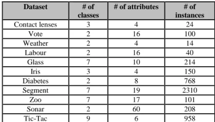
Table 1:UCI data sets characteristics Dataset # of classes # of attributes # of instances Contact lenses 3 4 24 Vote 2 16 100 Weather 2 4 14 Labour 2 16 40 Glass 7 10 214 Iris 3 4 150 Diabetes 2 8 768 Segment 7 19 2310 Zoo 7 17 101 Sonar 2 60 208 Tic-Tac 9 6 958
Input: The classifier CL, a test data Ts
Output: A classified test data for each instance in Ts do
for each rule ri in the classifier R do
if<ri, body>⊂ <ti, items>
assignri class to ti
else if <ri, any item>⊂< ti, items>
assignriclass to ti
else
assign default class to ti
end if end for end for
Fig. 3 Class allocation procedure of DRI algorithm Input: The Complete set of CARsR
Output: Sorted CARsR’
Given two rule, rm and rn, rm precedes rnif :
1.The expected accuracy of rm is larger than that of rn 2.The expected accuracy values of rm and rn are similar,
but the frequency of rm is larger than that of rn 3.The expected accuracy and frequency values of rm and
rn are similar, but rmbody frequency is larger than that of than rm
4.When all above criteria are the same for rm and rn then the choice is arbitrary
Fig. 2 Rule sorting of DRI algorithm
4.2TEST DATA CLASS ALLOCATION STEP
For a test data ti, the DRI algorithm goes over the sorted rules
in the primary classifier and the first rule having common items with ti classifies it. This means that all items in the fired
rule body must be contained in ti. In case no rule in the
primary classifier is found, the DRI moves on to the secondary classifier and applies the same procedure. In those cases when no rules are found in both primary and secondary classifiers the DRI algorithm will take on the first partial matching rule. By partially we mean an item of the rule’s body is matching an item in ti. DRI class allocation procedure surely minimises the
utilisation of the default class almost to no use at all. This should positively affect the overall classification accuracy of the classifier. Figure 3 displays the proposed class allocation procedure.
4.3DRI VS OTHER RI ALGORITHMS
PRISM based methods in data mining, such as Parallel Prism developed to improve PRISM’s limited output quality and efficiency in finding the rules. This section highlights the primary distinctions between the current proposed method and those that are PRISM based:
Unlike PRISM, the DRI algorithm generates perfect rules besides high coverage near perfect rules (low error rules). This results in less number of perfect rules in the primary classifier and allows other good rules to play a role in the classification phase of test data, which eventually reduces the use of the default class rule.
There is no rule sorting in PRISM and its successors whereas DRI favours among rules based on three new criteria in RI.
DRI algorithm uses two new thresholds named freq and
Rule_Strength to minimise the search space of items while constructing the rules. This makes the process of rule discovery more efficient.
PRISM utilises a static expected accuracy for each item associated with the class that have been computed once from the training data set during the first scan. On the other hand, DRI enables each item to have dynamic expected accuracy and frequency that often changes when a rule is derived. This ensures that each item has its true data representation while building the classifier.
5. DATA AND EXPERIMENTAL RESULTS
Table 1 displays the details of each data set used in the experiments. Different evaluation criteria are used to conduct the experiments and the results are analysed using:
Classification accuracy (%).
Number of rules particularly between DRI and PRISM algorithms
Different classification algorithms in data mining have been chosen to evaluate the general performance of the DRI algorithm with respect to classifiers predictive accuracy and rules. The majority of the chosen algorithms fall under the category of RI and these are RIPPER and PRISM. In addition, we have selected a known DT algorithm called C4.5 to further evaluate DRI. The reason for picking these algorithms is due to the fact that most of them employ similar learning methodology to DRI with the exception of C4.5, which uses information theory measure based on Entropy to build a DT classifier.
The experiments of the proposed algorithm have been conducted using a Java prototype whereas all remaining algorithms have been tested on WEKA (WEKA, 2012). WEKA is an open source Java based platform that was developed at the University of Waikato, New Zealand. It contains different implementations and evaluation measures of data mining and machine learning methods for tasks including classification, clustering, regression, association rules and feature selections. All experiments have been conducted on a computing machine with a 1.7 GHz processor.
The average accuracy produced by the considered algorithm on the 10 UCI data sets is displayed in Figure 4. It is clear that the DRI algorithm performed on average extremely well when compared to RIPPER and PRISM RI algorithms: average 1.51% and 4.58% higher accuracy than RIPPER and PRISM algorithms respectively. This gain has been resulted from the dynamic rules generated by this algorithm and it is a
Fig. 4 Average classification accuracy (%) for the considered algorithms on the UCI data sets
71.00% 72.00% 73.00% 74.00% 75.00% 76.00% 77.00% 78.00% 79.00% 80.00%
RIPPER % C4.5 % DRI% PRISM %
Fig. 5 The classification accuracy (%) for the considered algorithms on the10 UCI data sets
0.00% 20.00% 40.00% 60.00% 80.00% 100.00% 120.00% RIPPER % C4.5 % DRI% PRISM %
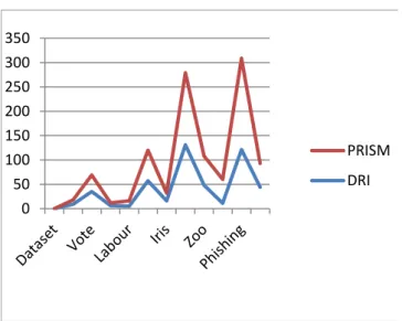
Fig. 6 The classifier size of PRISM and DRI algorithms on the data sets
0 50 100 150 200 250 300 350 PRISM DRI
consequence of keeping the highest fittest rules besides the perfect rules as this leads to improvement of the predictive power of DRI. On the other hand, DT algorithm C4.5 has slightly higher classification accuracy on overage that the proposed algorithm: average 0.67% higher accuracy. This can be considered good indeed because of the high predictive power of C4.5 besides the excessive pruning that are used by this algorithm during the process of constructing the classifier. The fact that DRI is competitive in regards to accuracy to C4.5 and derive on average higher predictive classifiers than its own kind is an achievement that deserves highlighting.
We have further evaluated the proposed algorithms per UCI data set and compared its predictive with the same three classification algorithms. Figure 5 shows the classification accuracy of all algorithms used in the experiments. It is worth noting that DRI outperformed most of the considered classification algorithms on the UCI data sets used in the experiments. In particular, the won-lost-tie record of DRI against RIPPER, PRISM and C4.5 are 6-4-0, 7-1-2, and3-1-6 respectively. The new rule evaluation method of DRI impacted positively on the classification performance of this algorithm by only allowing rules that are statistically fit to participate in the classifier. These rules are the ones utilised during class prediction step.
The number of rules in the classifiers produced by PRISM and DRI algorithms is depicted in Figure 6. PRISM generates on average larger classifiers than the DRI algorithm, which is due to the fact that PRISM has no pruning strategies at all. Dynamic update of candidate items when rules are generated results in a reduction of the search space of the items and therefore a lower number of candidate strong items are present. In other words, the removing of the overlapping among rules in the training instances when each rule is generated has also a positive impact on the classifiers size. In particular, DRI ensures that all candidate strong items expected accuracies as well as frequencies are amended on the fly whenever a rule gets produced, which definitely minimises the available numbers of candidate strong items for the next rules.
6. Conclusions
Rule Induction (RI), especially the PRISM algorithm, has few substantial issues including the production of only perfect rules (100% expected accuracy) and ignoring rules with high training data coverage. In respond to the above raised issue we proposed in this article a dynamic rule induction strategy (DRI) that utilise two threshold values to reduce the search space and to guarantee the production of not only perfect rules but also high quality rules. Moreover, DRI discards all data instances when a rule is generated and amends the frequencies of all remaining candidate items that appeared in the removed instances. This indeed makes fairer rules since the actual rules’ frequencies are incrementally updated rather computed once from the original training data set. Experimental results using ten UCI data sets have been conducted using different RI algorithms. The results revealed that DRI algorithm is highly competitive with respect to classification accuracy to PRISM, RIPPER and C4.5 algorithms. Moreover, DRI consistently produced less number of rules than PRISM. In future, we intend to extend DRI to deal with unstructured data set in order to handle the challenging problem of multi-label classification.
References
[1] Abdelhamid N., and Thabtah F. (2014) Associative Classification Approaches: Review and Comparison. Journal of Information and Knowledge Management (JIKM), 13, 1450027.Sept 2014. Worldscinet.
[2] Abdelhamid N., Ayesh A., F Thabtah (2014) Phishing detection based Associative Classification data mining.Expert Systems with Applications 41 (13), 5948-5959.
[3] Abdelhamid N., Ayesh A., Thabtah F., Ahmadi S., Hadi W (2012) MAC: A multiclass associative classification algorithm. To be published in the Journal of Information and Knowledge Management (JIKM). 11 (2), pp. 1250011-1 - 1250011-10. WorldScinet.
[4] Cendrowska, J. (1987) PRISM: An algorithm for inducing modular rules. International Journal of Man-Machine Studies, Vol.27, No.4, 349-370.
[5] Frank, E., and, Witten, I. (1998) Generating accurate rule sets without global optimisation. Proceedings of the Fifteenth International Conference on Machine Learning, (p. . 144–151). Madison, Wisconsin.
[6] Merz, C., and Murphy, P. (1996) UCI repository of machine learning databases. Irvine, CA, University of California, Department of Information and Computer Science.
[7] Mohammad RM, Thabtah F, McCluskeyL (2013) Predicting phishing websites based on self-structuring neural network. Neural Computing and Applications, 1-16 (2013)
[8] Quinlan, J. (1993) C4.5: Programs for machine learning. San Mateo, CA: Morgan Kaufmann.
[9] Rameshkumar, K., Sambath, M. and Ravi, S. (2013) Relevant association rule mining from medical dataset using new irrelevant rule elimination technique. Proceedings of ICICES ,300-304.
[10] Stahl F., and Bramer M. (2008) P-Prism: A Computationally Efficient Approach to Scaling up Classification Rule Induction (2008) Artificial Intelligence in Theory and Practice II, IFIP – The
International Federation for Information
Processing Volume 276, 2008, pp 77-86.
[11] Thabtah F., Hammoud S., Abdeljaber Hussein (2015) Parallel Associative Classification Data Mining Frameworks Based MapReduce. Journal of Parallel Processing Letter, 25 (02), 1550002.World Scientific. [12] Thabtah F., Hammoud S (2013) MR-ARM: A
MapReduce Association Rule Mining.Journal of Parallel Processing Letter, 23 (3) 1-22, 1350012.World Scientific.
[13] Thabtah, F., Cowling, P., and Peng, Y. (2004) MMAC: A new multi-class, multi-label associative classification approach. Proceedings of the Fourth IEEE International Conference on Data Mining (ICDM ’04), 217-224. [14] Thabtah, F. (2005) Rules Pruning in Associative
Classification Mining. Proceedings of the IBIMA conference, (pp. 101-107). Cairo, Egypt.
[15] Yin X., Han J. (2003) CPAR: Classification based on predictive association rule. Proceedings of the SIAM International Conference on DataMining -SDM, 369-376.
[16] Witten, I., and Frank, E. (2005) Data mining: practical machine learning tools and techniques with Java implementations. San Francisco: Morgan Kaufmann.