Sparse reduced-rank regression for imaging genetics studies: models and applications

(1)

genetics studies: models and applications

A thesis presented for the degree of Doctor of Philosophy of Imperial College

by

Maria Vounou

Department of Mathematics Imperial College

180 Queen’s Gate, London SW7 2BZ

(2)

2

I certify that this thesis, and the research to which it refers, are the product of my own work, and that any ideas or quotations from the work of other people, published or otherwise, are fully acknowledged in accordance with the standard referencing practices of the discipline.

(3)

Copyright

Copyright in text of this thesis rests with the Author. Copies (by any process) either in full, or of extracts, may be made only in accordance with instructions given by the Author and lodged in the doctorate thesis archive of the college central library. Details may be obtained from the Librarian. This page must form part of any such copies made. Further copies (by any process) of copies made in accordance with such instructions may not be made without the permission (in writing) of the Author.

The ownership of any intellectual property rights which may be described in this thesis is vested in Imperial College, subject to any prior agreement to the contrary, and may not be made available for use by third parties without the written permission of the University, which will prescribe the terms and conditions of any such agreement. Further information on the conditions under which disclosures and exploitation may take place is available from the Imperial College registry.

(4)

4

To my grandfather,

(5)

Abstract

We present a novel statistical technique; the sparse reduced rank regression (sRRR) model which is a strategy for multivariate modelling of high-dimensional imaging responses and genetic predictors. By adopting penalisation techniques, the model is able to enforce spar-sity in the regression coefficients, identifying subsets of genetic markers that best explain the variability observed in subsets of the phenotypes. To properly exploit the rich structure present in each of the imaging and genetics domains, we additionally propose the use of several structured penalties within the sRRR model. Using simulation procedures that ac-curately reflect realistic imaging genetics data, we present detailed evaluations of the sRRR method in comparison with the more traditional univariate linear modelling approach. In all settings considered, we show that sRRR possesses better power to detect the deleterious genetic variants. Moreover, using a simple genetic model, we demonstrate the potential benefits, in terms of statistical power, of carrying out voxel-wise searches as opposed to extracting averages over regions of interest in the brain. Since this entails the use of phe-notypic vectors of enormous dimensionality, we suggest the use of a sparse classification model as a de-noising step, prior to the imaging genetics study. Finally, we present the application of a data re-sampling technique within the sRRR model for model selection. Using this approach we are able to rank the genetic markers in order of importance of as-sociation to the phenotypes, and similarly rank the phenotypes in order of importance to the genetic markers. In the very end, we illustrate the application perspective of the pro-posed statistical models in three real imaging genetics datasets and highlight some potential associations.

(6)

6

Acknowledgements

I would first like to thank my supervisor, Dr Giovanni Montana, who has guided me and supported me throughout this procedure more than what I should have expected. Without his constant motivation, enthusiasm and his valuable assistance this work would have never been accomplished. Special thanks go to my second supervisor Dr Tom Nichols who has introduced me to this exciting multidisciplinary field of imaging genetics and helped me adjust by sharing his expertise in the area. My appreciations also go to a number of people, especially Eva Janousova, Dr Becky Inkster and Dr Eva Strijbis, with whom I have col-laborated on several projects during these years. Many thanks also go to GlaxoSmithKline (GSK) and the Engineering and Physical Sciences Research Council (EPSRC) who have provided financial support for this thesis.

A big thank you goes to my friend Ioannis Phinikettos who has been my officemate and an excellent support. I would also like to give my warmest thanks to my family, especially my mother Emmelia, my father Christos and my sister Stephanie, who have all contributed to this achievement through their constant psychological support and love. I would finally like to express my deepest gratitudes to Timon Kotsapas, who stood next to me all the way through, his encouraging words and love is what kept me going.

(7)

List of Figures

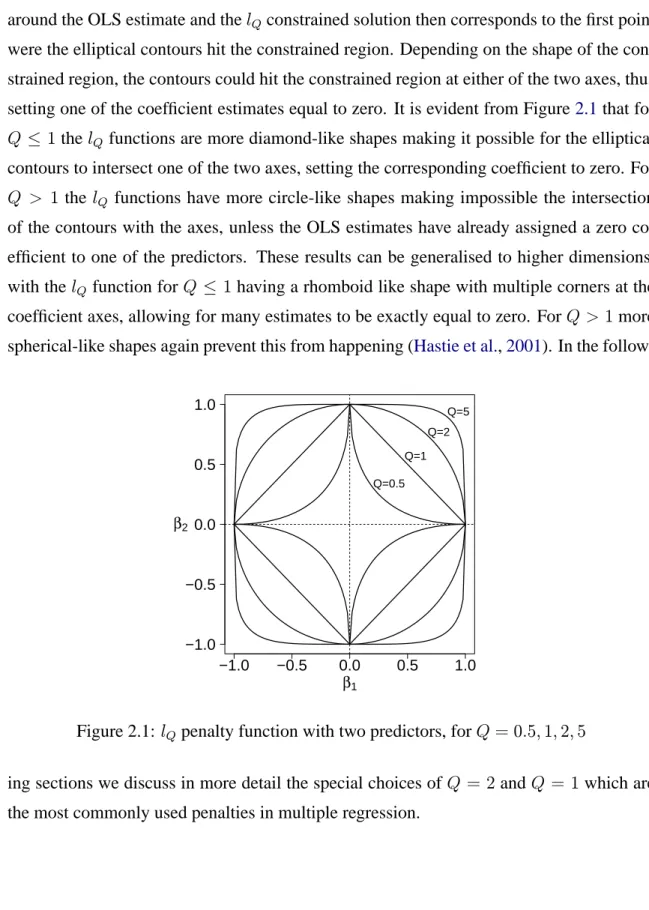
2.1 lQ penalty function with two predictors, forQ= 0.5,1,2,5 . . . 32

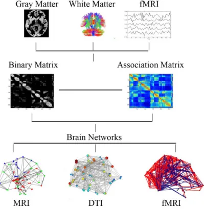
3.1 Illustration of the MMLR and sRRR models. . . 58 3.2 Schematic illustration of brain networks constructed from structural MRI,

DTI or fMRI data. In each case, an association matrix is first constructed with entries representing the weights connecting two regions in the brain. This can also be binary representing the existence or absence of an asso-ciation. A corresponding graphical representation, where brain regions are represented by nodes in the graph, and the links between two regions are represented by edges, is shown. The figure was adapted from Bassett and Bullmore(2009). . . 65 3.3 Schematic illustration of a network between the APOE gene and 9 other

genes. The links connecting the genes represent either pathway-related links (green lines) or physical interaction links (blue lines). The plot was created using the GeneMANIA software (http://www.genemania.org/) . . . 67

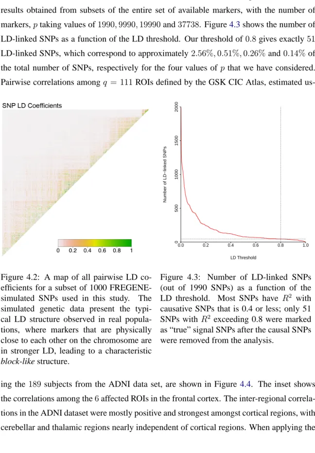
4.1 Sagittal, coronal and axial views of the GSK CIC Atlas defining 111 re-gions of interest.. . . 75 4.2 A map of all pairwise LD coefficients for a subset of 1000

FREGENE-simulated SNPs used in this study. The FREGENE-simulated genetic data present the typical LD structure observed in real populations, where markers that are physically close to each other on the chromosome are in stronger LD, lead-ing to a characteristic block-like structure. . . . 78 4.3 Number of LD-linked SNPs (out of 1990 SNPs) as a function of the LD

threshold. Most SNPs haveR2_{with causative SNPs that is 0.4 or less; only}

51 SNPs withR2 _{exceeding 0.8 were marked as “true” signal SNPs after}

the causal SNPs were removed from the analysis. . . 78 4.4 All pairwise correlations among q = 111 ROIs defined by the GSK CIC

Atlas and estimated usingn = 189subjects from the ADNI data set. The inset shows the correlations among the6affected ROIs in the frontal cor-tex: left and right each of precentral gyrus (41, 42), anterior dorsolateral prefrontal cortex (43, 44), posterior dorsolateral prefrontal cortex (45, 46). . 79

(10)

LIST OF FIGURES 10

4.5 Rank trace plot. Thex-axis representsΔ ˆC, and they-axis representsΔˆS,

as described in Section 3.1.1. For each reduced-rank r ranging from 0

(top-right corner) toR (bottom-left corner) there is a corresponding point

(Δ ˆC(r),ΔˆS(r))along the curve. A suitable rank R

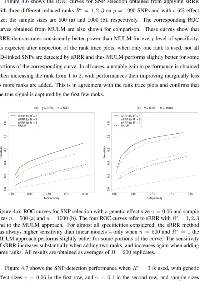
∗ _{can be selected by} locating the point at which curvature is maximal – in this example, based onγ = 0.06andn= 1000, this point corresponds toR∗ _{= 4}_{and is marked} by the vertical and horizontal lines. However, for all of our experiments, we use R∗ _{= 3} _{as we have empirically observed that this choice gives a} satisfactory performance and the gain of including a further rank is only minimal. . . 80 4.6 ROC curves for SNP selection with a genetic effect size γ = 0.06 and

sample sizes n = 500(a) and n = 1000(b). The four ROC curves refer to sRRR with R∗ = 1,2,3 and to the MULM approach. For almost all specificities considered, the sRRR method has always higher sensitivity than linear models – only whenn= 500andR∗ _{= 1}_{the MULM approach} performs slightly better for some portions of the curve. The sensitivity of sRRR increases substantially when adding two ranks, and increases again when adding three ranks. All results are obtained as averages ofB = 200

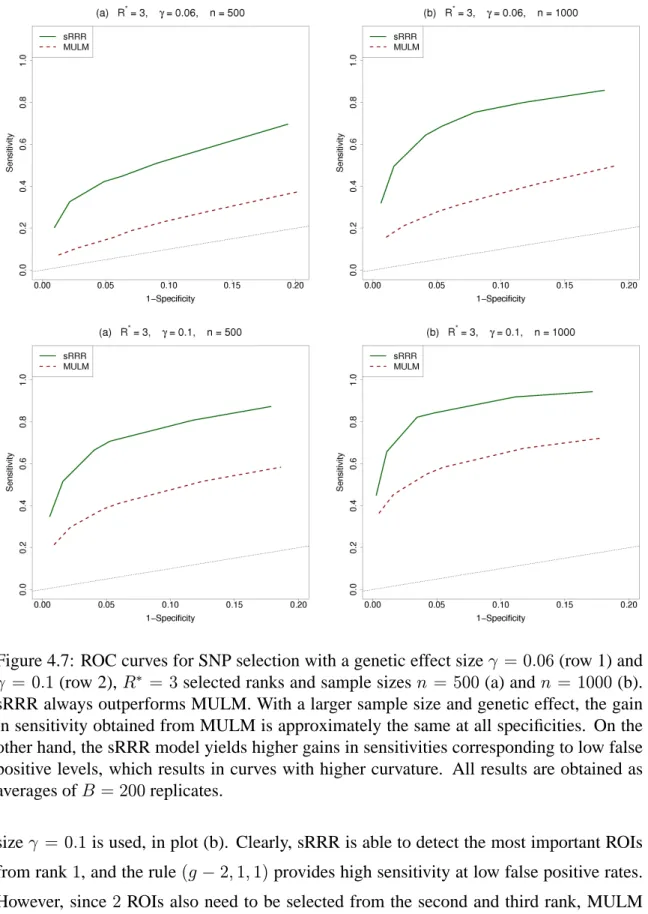
replicates. . . 81 4.7 ROC curves for SNP selection with a genetic effect size γ = 0.06 (row

1) and γ = 0.1 (row 2), R∗ _{= 3} _{selected ranks and sample sizes} _n ₌

500 (a) and n = 1000 (b). sRRR always outperforms MULM. With a larger sample size and genetic effect, the gain in sensitivity obtained from MULM is approximately the same at all specificities. On the other hand, the sRRR model yields higher gains in sensitivities corresponding to low false positive levels, which results in curves with higher curvature. All results are obtained as averages ofB = 200replicates. . . 83 4.8 Comparison of sRRR and MULM for large p: shown here is the ratio of

SNP sensitivities (sRRR/MULM) as a function of the total number of SNPs included in the study. The genetic effect size isγ = 0.06,R∗ _{= 3}_selected ranks and sample size n = 1000. All results are obtained as averages of B = 200 replicates. This result suggests that the potential power gain coming from the sRRR model can be much higher in GWAs when the number of available SNPs is much more than 40k. For further details see Table 4.1. . . 84 4.9 ROC curves for ROI selection: n = 500, R∗ _{= 3}_{and genetic effect size}

(a)γ = 0.06and (b)γ = 0.1. For the latter genetic effect sRRR has worse sensitivity for lower false positive rates, and the MULM approach shows good performance. Notably, for the lower genetic effect, sRRR outper-forms MULM. All results are obtained as averages ofB = 200replicates. . 86

(11)

4.10 Sagittal view of a color-coded atlas of the brain. A ROIk (in dark yellow) has been picked to illustrate two possible scenarios: (a) all the voxels within the ROI are signal voxels, (b) the signal is gathered in a smaller subregion of the ROI. The signal intensity is represented by shades of black. . . 87 4.11 SNP, ROI and voxel sensitivity (rows 1-3) while varying the percentage

of signal voxels,tk, within the affected ROI, for the three methods; group

Lasso (group- black full line), sparse group Lasso (sgroup- red dashed line), Lasso for ROI averages (averages- dotted-dashed green line). The left and right columns correspond to results with the per-voxel SNR fixed to5%and10%, respectively. . . 93 5.1 Selection probabilities for the predictors (row 1) and the responses (row 2)

in rank 1,2 and 3 analyses (from left to right). Simulated genetic markers and phenotypes that are associated in the first and second ranks are illus-trated in red and green respectively, whereas the noise variables are denoted by black dotted lines. . . 108 5.2 Stability selection plots for SNPs (row 1) and ROIs (row 2) of the rank

1 and 2 (left and right) of the sRRR model. The associated variables are illustrated by red lines, whereas the noise variables are illustrated in black dotted lines. . . 110 5.3 Stability selection plots for the SNPs (left) and for the ROIs (right), of rank

1 of the sRRR model with randomisation. The associated variables are illustrated by red lines, whereas the noise variables are illustrated in black dotted lines. . . 111 5.4 Stability selection plots for SNPs (left plot) and ROIs (right plot) of rank

1 of the sRRR model. The associated variables are illustrated by red lines, whereas the noise variables are illustrated in black dotted lines. . . 112 6.1 Pairwise correlations between the 7 phenotypes. NBV is highly correlated

with NGMV and NWMV, whereas the other pairwise phenotype correla-tions are low or moderate.. . . 123 6.2 Selection probabili ties for the SNPs (left plot) and phenotypes (right plot)

for the rank 1 analysis of the sRRR model. For the SNP probabilities, SNPs belonging in the candidate group are illustrated in red and a horizontal line on the 0.5 probability threshold is illustrated in dark blue. For the phenotype probabilities, each phenotype is denoted by a different colour according to the legend. . . 125

(12)

LIST OF FIGURES 12

6.3 Selection probabilities for the SNPs (top row) and phenotypes (bottom row) for the rank 1 (left plot) and rank 2 (right plot) analysis of the sRRR model. For the SNP probabilities, SNPs belonging in the candidate group are il-lustrated in red and a horizontal line on the 0.5 probability threshold is illustrated in dark blue. For the phenotype probabilities, each phenotype is denoted by a different colour according to the legend in the right plot. . . . 131 6.4 Schematic illustration of the ordering of genes in our study. The number of

SNPs available for each gene are given in the bracket. . . 138 6.5 Pairwise correlations of the 1439 voxels from the 3 ROIs: IPS, amygdala

(AMG) and OFC. Relatively high correlations are observed between sub-sets of voxels from AMG and OFC, whereas IPS appears to be mostly uncorrelated with the other two regions. . . 140 6.6 Selection probabilities for all 98 SNPs for the rank 1 (left) and rank 2 (right)

analysis of the sRRR model. SNPs belonging in the key hypothesised genes LIMK1, CLIP2, GTF2I and GTF2IRD1 are illustrated in red. A horizontal line on the 0.5 probability threshold is illustrated in dark blue. . . 143 6.7 Selection probabilities for all 1439 voxels for the rank 1 (left) and rank

2 (right) analysis of the sRRR model. Voxels belonging in OFC, IPS and amygdala regions are illustrated in blue, red and green colours respectively. A horizontal line on the 0.5 probability threshold is illustrated in grey. . . . 143 7.1 Two-dimensional representation of all the subjects obtained by

multidi-mensional scaling of the imaging signatures identified by penalised LDA: AD versus CN (left), P-MCI versus CN (middle) and P-MCI versus S-MCI (right). The blue crosses refer to theHclass, i.e. the CN individuals in the left and middle plots and the S-MCI individuals in the right plot. The red triangles refer to the D class, i.e. AD patients in the left and the P-MCI patients in the middle and right plots.. . . 155 7.2 Brain images showing the results from the penalised LDA analysis of the

AD versus CN comparison. The selected voxels are illustrated in yellow for the 3 planes of view of the brain (coronal, sagittal and axial from left to right). Illustrations of the actual selection probabilities are shown in colour scale in the insets below. . . 157 7.3 Brain images showing the results from the penalised LDA analysis of the

P-MCI versus CN comparison. The selected voxels are illustrated in yellow for the 3 planes of view of the brain (coronal, sagittal and axial from left to right). Illustrations of the actual selection probabilities are shown in colour scale in the insets below. . . 157

(13)

7.4 Brain images showing the results from the penalised LDA analysis of the P-MCI versus S-MCI comparison. The selected voxels are illustrated in yellow for the 3 planes of view of the brain (coronal, sagittal and axial from left to right). Illustrations of the actual selection probabilities are shown in colour scale in the insets below.. . . 158 7.5 Stability selection probabilities for the AD versus CN analysis for ranks 1,

2 and 3 (from left to right). Lines corresponding to SNPs with (maximum) selection probabilities greater than or equal to the threshold π_x = 0.5are illustrated in red. The probability threshold is illustrated by a horizontal blue line atΠˆxk = 0.5. . . 166

7.6 Stability selection probabilities for the P-MCI versus CN analysis for ranks 1, 2 and 3 (from left to right). Lines corresponding to SNPs with (maxi-mum) selection probabilities greater than or equal to the thresholdπx = 0.5

are illustrated in red. The probability threshold is illustrated by a horizontal blue line atΠˆxk = 0.5. . . 166

7.7 Stability selection probabilities for the P-MCI versus S-MCI analysis for ranks 1, 2 and 3 (from left to right). Lines corresponding to SNPs with (maximum) selection probabilities greater than or equal to the threshold πx = 0.5are illustrated in red. The probability threshold is illustrated by a

(14)

14

List of Tables

4.1 False positive rate and power comparisons: pis the total number of avail-able SNPs; g is the target number of selected SNPs; αsRRR and αM U LM

are the false positive rates (1-specificity) achieved by sRRR and MULM, respectively. πsRRR and πM U LM are the power (sensitivity) achieved by

sRRR and MULM, respectively. In sRRR, we set R∗ _{= 3} _{and use the} uniform allocation rule (g/3, g/3, g/3). Note that due to possible redun-dancies between the sets of g/3SNPs selected from each rank, the actual number of ‘unique’ SNPs, selected over all ranks, is usually somewhat less than the target numberg, illustrated in this table. For any value ofg, as the total number of SNPs in the study gets larger, the ratioαsRRR/αM U LM

re-mains constant and always below1, indicating that sRRR achieves smaller false positive rate, while the ratioπsRRR/πM U LM is always above1,

indi-cating that sRRR achieves higher power. Remarkably, the relative power of sRRR compared to MULM gets larger as pincreases, for any value of g, but particularly so for smaller values ofg. The sample size isn = 1000

and the genetic effect isγ = 0.06. All results are obtained as averages of B = 200replicates. . . 85 5.1 Number of selected SNPs,_|Sˆx|, with a probability thresholdπx = 0.5and

the subsequent numbers of true and false positives_|Sˆx∩Sx|and|Sˆx∩Nx|,

for rank 1 and 2 of the sRRR model. Similarly, the number of selected ROIs,_|Sˆy|, withπy = 0.5and the corresponding numbers of true and false

positives_|Sˆ_y _∩S_y_|and_|Sˆ_y_∩N_y_|. . . 109 6.1 Number of SNPs for each group of candidate (cand), negative control

(neg) and positive control (pos), for each experiment (epigenetic and glu-tamate). The final, total, number of SNPs included in the analysis is also provided (tot). . . 124 6.2 Sample size (nG), number of males (male), mean age at baseline (age-bl),

mean disease duration in months (duration) for each disease class (RRMS and SPMS). The corresponding standard deviations are given in brackets. . 124

(15)

6.3 The top 6 SNPs and the phenotypes from the sRRR rank 1 epigenetic anal-ysis, ranked according to their selection probabilities. For each marker also provided are: the corresponding gene annotation where applicable, the chromosome, the MAF, the HWEp-value and the selection probability. SNPs and the corresponding genes belonging in the candidate epigenetic group are denoted in italics.. . . 125 6.4 The top 6 SNPs from the Lasso analysis of the NBV, ΔT2LL, NWMV,

PBVC and NGMV that scored highly on the corresponding sRRR analysis. In each analysis the SNPs are ranked according to their selection prob-abilities and for each marker also provided are: the corresponding gene annotation where applicable, the chromosome, the MAF, the HWEp-value and the selection probability. SNPs and the corresponding genes belonging in the candidate epigenetic group are denoted in italics. . . 127 6.5 The top 6 SNPs from the MULM analysis of NBV,ΔT2LL, NWMV, PBVC

and NGMV that scored highly on the corresponding sRRR analysis. In each analysis the SNPs are ranked according to theirp-values and for each marker also provided are: the corresponding gene annotation where appli-cable, the chromosome, the MAF and the HWE p-value. SNPs and the corresponding genes belonging in the candidate epigenetic group are de-noted in italics. . . 128 6.6 The top SNPs (with selection probabilities_≥0.4) and the phenotypes from

the sRRR rank 1 and 2 glutamate analysis, ranked according to their selec-tion probabilities. For each marker also provided are: the corresponding gene annotation where applicable, the chromosome, the MAF, the HWE p-value and the selection probability. SNPs and the corresponding genes belonging in the candidate glutamate group are denoted in italics.. . . 130 6.7 The top 6 SNPs from the Lasso analysis of NBV, NGMV, NWMV and

ΔT2LL that scored highly on the corresponding sRRR analysis. In each analysis the SNPs are ranked according to their selection probabilities and for each marker also provided are: the corresponding gene annotation where applicable, the chromosome, the MAF, the HWEp-value and the selection probability. SNPs and the corresponding genes belonging in the candidate glutamate group are denoted in italics. . . 133 6.8 The top 6 SNPs from the MULM analysis of NBV, NGMV, NWMV and

ΔT2LL that scored highly on the corresponding sRRR analysis. In each analysis the SNPs are ranked according to theirp-values and for each marker also provided are: the corresponding gene annotation where applicable, the chromosome, the MAF and the HWEp-value. SNPs and the genes belong-ing in the candidate glutamate group are denoted in italics. . . 134 6.9 The three ROIs, IPS, amygdala (AMG) and OFC and the number of voxels

(16)

LIST OF TABLES 16

6.10 The top ten SNPs ranked according to their selection probabilities for rank 1 and 2 of the sRRR analysis. For each marker also provided are: the cor-responding gene annotation, the MAF, the HWEp-value and the selection probability. . . 142 7.1 Number of individuals included in each experiment (n), corresponding

number of individuals in each class (nH and nD), and the final number

of SNPs that survived quality control in each class (p). . . 150 7.2 Sample size (nG), number of males (male), mean age at baseline (age-bl),

mean MMSE score at baseline (msse-bl), mean age difference at up (age-fu) and mean absolute difference in the MMSE score after follow-up (mmse-fu) for each disease class. The corresponding standard devia-tions are given in brackets. . . 150 7.3 Number of selected voxels (vox) and10-fold cross validated performance

measures in%- accuracy (acc), sensitivity (sen) and specificity (spe) -using a SVM classifier with Gaussian kernel. . . 155 7.4 The top ten SNPs with selection probabilities _≥ 0.5 (ranked according

to their selection probabilities) for rank 1, 2 and 3 of the AD versus CN sRRR analysis. For each marker also provided are: the corresponding gene annotation where applicable, the chromosome, the MAF, the HWEp-value and the selection probability. . . 163 7.5 The top ten SNPs with selection probabilities _≥ 0.5(ranked according to

their selection probabilities) for rank 1, 2 and 3 of the P-MCI versus CN sRRR analysis. For each marker also provided are: the corresponding gene annotation where applicable, the chromosome, the MAF, the HWEp-value and the selection probability. . . 164 7.6 The top ten SNPs with selection probabilities _≥ 0.5(ranked according to

their selection probabilities) for rank 1, 2 and 3 of the P-MCI versus S-MCI sRRR analysis. For each marker also provided are: the corresponding gene annotation where applicable, the chromosome, the MAF, the HWEp-value and the selection probability. . . 165

(17)

List of Publications

[1] Vounou, M., Nichols, T., and Montana, G. (2010). Discovering genetic associations with high-dimensional neuroimaging phenotypes: A sparse reduced-rank regression approach. NeuroImage, 53(3):1147-1159.

[2] Vounou, M. and Montana, G. (2010). Genetic association mapping with imaging phenotypes. In International Young Scientists Conference: “Perspectives for

Devel-opment of Molecular and Cellular Biology II”.

[3] Vounou, M., Janousova, E., Wolz, R., Stein, J. L., Thompson, P. M., Rueckert, D., and Montana, G. (2011). Sparse reduced-rank regression detects genetic associations with voxel-wise longitudinal phenotypes in Alzheimer’s disease. NeuroImage. In press.

[4] Inkster, B., Strijbis, E. M. M., Vounou, M., Kappos, L., Radue, E. W., Matthews, P. M., Uitdehaag, B., Barkhof, F., Polman, C. H., Montana, G., and Geurts, J. J. G. (2011). Histone deacetylase gene variants predict brain volume changes in multiple sclerosis. submitted to Neurobiology of Aging.

[5] Strijbis, E. M. M., Inkster, B., Vounou, M., Kappos, L., Radue, E. W., Matthews, P. M., Uitdehaag, B., Barkhof, F., Polman, C. H., Montana, G., and Geurts, J. J. G. (2011). Glutamate gene polymorphisms predict brain volume changes in multiple sclerosis. submitted to Archives of Neurology.

[6] Inkster, B., Vounou, M., Wolz, R., Rueckert, D., and Montana, G. (2011). Ki-nomic screening for gene variants that predict brain atrophy in Alzheimer’s disease.

(18)

18

Chapter 1 Introduction

1.1 Introduction to imaging genetics

Most genetic association studies with neurological disorders to date are based on case-control designs, and as such they rely on a crude indicator of disease status. However, over the last few years, interest has shifted towards imaging genetics studies that search for associations with intermediate phenotypes extracted from magnetic resonance

imag-ing (MRI) scans of the brain. Compared to a dichotomous disease indicator variable, an

imaging-based signature provides a richer quantitative characterisation of the disease at any given time. The identification of genetic markers that explain the disease-related variabil-ity observed in brain structure or function, as reflected in structural MRI or functional MRI (fMRI) scans, can have a great impact in uncovering the underlying disease mechanism and lead to potential treatments or preventions (Glahn et al.,2007;Thompson et al.,2010). The field of imaging genetics is currently catching up with the dramatic increase in the number of genome-wide association (GWA) studies that have been reported across many different disease areas, and that have been fuelled by recent technological improvements in genotyping and reductions in cost. The fundamental assumption that underlies the GWA approach is that extensive common variation in the human genome, as measured for exam-ple by single nucleotide polymorphisms (SNPs) or copy number variation (CNV) markers, contributes to the risk of most common disorders. Over the last few years, substantial in-ternational resources have been directed in an effort to better characterise human genetic

(19)

variation, for instance through the HapMap1 and the Genome 1000 projects2. The latest genotyping platforms enable the measurement of around 2.5 million SNP and CNV mark-ers (Lamy et al.,2011).

A number of population-based association studies with neuroimaging phenotypes have appeared in the literature over the last few years. Based on both the dimensionality of the phenotype being investigated and the size of the genomic regions being searched for asso-ciation, we attempt a broad classification of the existing imaging genetic studies into four main categories. Some studies can be classified as belonging to the candidate-phenotype,

candidate-gene association (CP-CGA) category, meaning that a specific gene or

chromo-somal region is tested for association with a typically low-dimensional phenotype. The as-sumption is that the particular quantitative phenotypes being measured are able to capture changes in the brain induced by the disease or other biological conditions being studied. An example of this approach is described byJoyner et al. (2009), who examine the poten-tial association between four summary brain structure measures and eleven SNPs, located in and around the MECP2 gene. They study two populations, one consisting of healthy controls and patients with psychotic disorders, and one consisting of healthy controls and patients with mild cognitive impairment and Alzheimer’s disease.

Other studies belong to the candidate-phenotype, genome-wide association (CP-GWA) category where again, the phenotype has been appropriately identified but the search for genetic variants has a much wider scope. An example is given by Potkin et al. (2009c), who use a brain imaging activation signal in the dorsolateral prefrontal cortex as the quan-titative trait reflecting schizophrenia dysfunction, and present a genome-wide study based on subjects with chronic schizophrenia and controls matched for age and sex.

The third category includes studies that have taken the opposite approach, and fall into the brain-wide, candidate-gene association (BW-CGA) class. In this case, the search for genetic variants is confined to specific chromosomal regions or genes of interest, but is extended to the entire brain by the means of very high-dimensional phenotypes, typically based on voxel-based morphometry (VBM) techniques.Filippini et al.(2009) describe one

1_{http://hapmap.ncbi.nlm.nih.gov}

(20)

1.1 Introduction to imaging genetics 20 such study, in which a whole-brain search for associations between the APOEε4 allele load and voxel-wise grey matter volume is carried out by testing for both additive and genotypic models in a population of patients with Alzheimer’s disease.

Currently, studies in imaging genetics are shifting towards the fourth category, the

brain-wide, genome-wide association (BW-GWA) paradigm, where both the entire genome

and entire brain are searched for non-random associations. A recent example is the study carried out by Stein et al. (2010). Here, a voxel-wise search for variants that influence brain structure in Alzheimer’s disease is performed, using approximately448000SNPs and around 31000voxels across the entire brain. Imaging genetics and especially BW-GWA studies commonly rely on high-dimensional phenotypes and genotypes. The assumption is that only a handful of quantitative traits (e.g. voxels or voxel clusters) may be found in a statistically meaningful association with a handful of genetic markers. The approach thus requires a statistical framework for the simultaneous identification of genomic regions and brain regions that are found to be in non-random association.

The most common approach in the literature of imaging genetics has been to fit an enor-mous number of univariate linear regression models, regressing each phenotype on each genetic marker one at a time. Hypothesis testing is then carried out by computing a test statistic for each one of the many possible genotype-phenotype pairs, and an experiment-wide significance level is attained by correcting for multiple testing. This approach, which we refer to as the mass-univariate linear modelling (MULM) approach, is appealing be-cause of its simplicity and bebe-cause the univariate regression models can be easily fitted even when only small sample sizes are available. However, it has two major limitations:

(a) each genotype is independently tested for association with one phenotype at a time

(b) each phenotype is independently tested for association with one genotype at a time

Common complex diseases are expected to be caused by multiple genetic markers, each contributing a small amount to the effect present on the disease phenotypes, rather than by single mutations with large effects (Stranger et al., 2011; Zondervan and Cardon, 2004). Because of (a), the MULM approach is unable to capture possible cumulative effects from multiple markers that jointly contribute to explain the phenotypic variability, and therefore may not fully exploit the signal that is present in the data. In fact, by using a multi-locus

(21)

penalised regression model, a boost in power compared to the univariate approach has been recently reported in detecting GWA associations with temporal lobe and hippocampal volumes (Kohannim et al.,2011).

Moreover, (b) implies that the MULM approach does not fully exploit the additional power gains that are expected when using multiple quantitative phenotypes. Correlated phenotypes, and especially voxel-wise phenotypes that have strong structural connections, are expected to share some common genetic variation; see, for instance,Eyler et al.(2011) andChiang et al.(2011) for recent twin studies demonstrating this point. In the latter study, a two-step strategy was adopted to boost the power to detect GWAs. Firstly, clusters of vox-els with strong pairwise genetic correlations (thus exhibiting strong genetic homogeneity) were identified, and subsequently their average values were used as phenotypes for the as-sociation study. In that sense, a model that fully accounts for the multivariate nature of the phenotypes can potentially yield higher statistical power due to a stronger association signal (Breiman,1996b;Breiman and Friedman,1997;Ferreira and Purcell,2009;Lounici et al.,2010).

Another major challenge in the framework of MULM is related to the need to deter-mine an experiment-wide significance level that accounts for the multiple testing problem. The family-wise error rate is routinely controlled by a Bonferroni correction (Hochberg and Tamhane,1987) and the false discovery rate can be controlled by procedures proposed byBenjamini and Hochberg(1995) andBenjamini and Yekutieli(2001). However, in the context of imaging genetics, the complex dependence structure among both genetic mark-ers and among phenotypes must be accounted for. For example,Stein et al.(2010) collapse inferences over the entire set of SNPs at each voxel by taking the minimump-value. Then, they correct for the effective dimensionality accounting for the linkage disequilibrium (LD) among the markers. Other approaches rely on computationally-intensive permutation pro-cedures, (see for examplePotkin et al.,2009b).

1.2 Thesis overview

In this thesis we attempt to address the shortcomings of the current imaging genetics proce-dures and propose alternative statistical strategies for identifying genetic associations with

(22)

1.2 Thesis overview 22 neuroimaging phenotypes. In particular, we propose the use of the sparse reduced-rank

regression (sRRR); a multivariate multiple regression technique that makes explicit use of

the multivariate structure of the response vector by assuming a low rank representation. By adopting penalisation techniques, the coefficients of the regression model are estimated to be sparse, effectively performing simultaneous genotype and phenotype variable selection. We suggest the use of several structural penalties that can take advantage of the specific data structures in imaging genetics, such as grouping structures of SNPs into genes or pathways and structural connections of voxels or regions in the brain. By framing the identification of genetic associations as a variable selection problem rather than one of hypothesis test-ing, there is no need to rely on multiple testing correction procedures. The fact that the model includes all available genetic markers and phenotypes also addresses the limitations due to both (a) and (b) above, and is thus expected to increase the power to detect true associations.

To compare the power of our method to that of the more conventional MULM ap-proach, we introduce a detailed simulation framework that associates a small number of markers with brain-wide phenotypes representing the average grey matter volume of

re-gions of interest (ROIs) in the brain. We use a realistic simulation of both genomic and

phenotypic variation to accurately reflect real imaging genetics datasets. Further realism is introduced by subsequently removing true causative markers from the study, so that genotype-phenotype associations can be detected only through markers that are in LD with these excluded markers. In all settings considered we show that sRRR has better power to detect the deleterious genetic variants.

In order to quantify the loss of statistical power that may potentially result when extract-ing ROI averages, we propose a simple mathematical framework comparextract-ing the

signal-to-noise ratio (SNR) from the two competing phenotypes: one based on individual voxels and

one based on ROI averages. Through these results we are able to formalise the intuition that a voxel-wise approach is to be preferred, provided that the majority of voxels considered as phenotypes are highly representative of the disease. We provide additional simulation ex-periments to demonstrate the power gains when using voxel-wise phenotypes, compared to using phenotypes representing ROI averages. Again we simulate realistic voxel-wise phe-notypes but use toy simulations for the genetic data so that we reduce the complexity in the

(23)

genotypic domain and focus on the comparison of the performance due to the phenotypes used.

The proposed sRRR model involves regularisation parameters responsible for genotype and phenotype selection which result in different estimated models. We combine the sRRR model with a data re-sampling technique, known as stability selection, for the purpose of model selection. This approach amounts to repeatedly fitting the model to sub-samples extracted from the data and estimating an importance measure of each variable based on its frequency of selection across the sub-sampling procedure. This enables us to rank the genetic markers in order of importance to the phenotypes and similarly rank the phenotypes in order of importance to the genetic markers. We also discuss some theoretical properties of this approach and suggest in future work, to look at the joint probabilities (how often each genotype-phenotype pair is selected) rather than the individual probabilities as an alternative approach.

Finally, we present three real data applications where we use the sRRR model combined with stability selection to highlight potential genetic associations with imaging measures. In all studies performed we highlight several possible genetic markers in association with the imaging phenotypes.

In the first application we perform two CP-CGA studies in a population of patients, with different disease levels of multiple sclerosis. In both studies we use the same disease-related phenotypic summary measures. The candidate genes were selected using prior knowledge; in the first study the genes were selected based on their critical role for epi-genetic regulation whereas in the second study the genes were selected based on their in-volvement in glutamate metabolism, both known to be critical for the disease.

Our second application is a CP-CGA study using a sample of healthy individuals, where we examine their genetic variations in a chromosomal region known to be deleted in pa-tients with William’s syndrome. Since brain dysfunction, as well as other disease symp-toms, observed in patients with this syndrome are directly linked to the deleted genetic material, genetic markers in that region are expected to be associated with similar dys-functions observed in the general population. For this study we use voxel-wise measures representing brain activation in three key brain regions, resulting from an fMRI experiment. Our third application is a voxel-wise BW-GWA study on a sample of Alzheimer’s

(24)

dis-1.3 Thesis structure 24 ease patients, patients with progressive and stable mild cognitive impairment, and healthy subjects. We perform three different experiments, where in each one we use two differ-ent groups of individuals (grouped according to disease status) to independdiffer-ently assess variations related to different stages of the disease. In this study brain-wide voxel-wise measurements, representing longitudinal changes from baseline and 24 month follow up MRI scans, are used as phenotypes. Based on our SNR results demonstrated earlier, we first apply a sparse classification approach, in particular a penalised linear discriminant analysis procedure, to identify a reduced set of voxels that best discriminate the two groups of individuals. These are then subsequently used for the imaging genetics studies.

1.3 Thesis structure

In Chapter 2 we provide a literature review on penalised regression techniques for vari-able selection in the context of multiple linear regression. In Chapter 3 we describe the reduced-rank regression model and discuss its connections with several other multivariate models. We then propose the sRRR model for performing simultaneous selection in both the imaging and genetic domains, and suggest a range of possible penalties to be used within this framework that are suitable for specific data structures characterising imaging genetics. The simulation experiments comparing the performance of sRRR and MULM are presented in Chapter 4. In the same chapter we demonstrate the analytical results on the SNR of ROI averages and voxel-wise phenotypes and provide the additional simula-tion experiments demonstrating this point. Part of the work from these chapters has been published in Neuroimage, see[1]in the list of publications.

In Chapter5we present the data re-sampling technique for model selection. The mul-tiple sclerosis study is presented in Chapter6. This work was a result from a collaboration with several people, including Dr. Becky Inkster who has been a research associate in Im-perial College, supervised by Dr. Giovanni Montana during November 2010 - April 2011 and Dr. Eva Strijbis from the Department of Neurology, VU University Medical Center in Amsterdam. Manuscripts from the two multiple sclerosis studies have been submitted to Neurobiology of Aging and Neurology, see[4]and[5]in the list of publications.

(25)

col-laboration with the group of Prof. Andreas Meyer-Lindenberg from the department of Psychiatry and Psychotherapy in University of Heidelberg in Germany. The corresponding work is currently being prepared for publication.

The penalised linear discriminant analysis for voxel filtering and the Alzheimer’s dis-ease study are presented in Chapter 7. This study was done in collaboration with Eva Janousova, who was a visiting student in Imperial College supervised by Dr. Giovanni Montana, during October 2010 - March 2011, Dr. Robin Wolz and Prof. Daniel Rueckert from the Department of Computing of Imperial College as well as Dr. Jason Stein and Prof. Paul Thompson from the Laboratory of Neuro Imaging, Department of Neurology, UCLA School of Medicine in USA. The work from this chapter has been submitted to Neuroimage, see[3]in the list of publications.

The conclusions and directions for further research are found in Chapter8.

Parts of the work presented in this thesis have been presented in a number of confer-ences as poster and oral presentations. In particular, I have presented posters in

• Multi-level and voxel-wide search for genetic associations with imaging phenotypes using penalized regression. 7th International Imaging Genetics Conference, Irvine, USA, 17-18 January, 2011

• Genome-wide Association Studies in Imaging Genetics: A Multivariate Approach. CIC Student Day, GSK Clinical Imaging Centre, 4 November, 2009.

• Genome-wide Association Studies in Imaging Genomics: A Multivariate Approach. 19th annual MASAMB workshop, Imperial College London, 2-3 April, 2009

• Genome-wide Association Studies in Imaging Genomics: A Multivariate Approach. 5th International Imaging Genetics Conference, Irvine, USA, 19-20 January 2009. (This poster has been awarded one of the two available ‘IIGC 2009 Travel Awards’)

I have also given a talk in

• Penalized Regression Strategies in Imaging Genetics. Creativity Lab, Imperial Col-lege, 9 February 2011.

Dr. Giovanni Montana has also given several invited talks on our work in the following conferences:

(26)

1.4 Notation 26 • Statistical models for genome-wide studies in neuroimaging genetics and

applica-tions. School of Computing, University of Singapore, 5 September, 2011

• Penalised regression strategies in imaging genetics studies. 7th International Imaging Genetics Conference, Irvine, USA, 17-18 January, 2011

• Genetic association mapping with imaging phenotypes. International YS Conference Perspectives for Development of Molecular and Cellular Biology II, 10-12 Novem-ber, 2010, Yerevan, Armenia (including a conference proceedings publication, see [2]in the list of publications)

• Genome-wise biomaker discovery in neuroimaging studies. PSI Biomarker (Statisti-cians in the Pharmaceutical Industry). Roche, Welwyn, UK. 5 November 2010 • Imaging genetics. Multivariate approaches: joint modeling. 16th Human Brain

Map-ping Conference, 6-10 June 2010, Barcelona.

• Sparse multivariate methods to study whole genome genotype-imaging phenotypes associations. Imaging Genetics Statistical Workshop, Oslo University. 11 June, 2009, Ulleval, Norway.

A contributed talk has also been given by Dr Giovanni Montana in

• Biomarker discovery in imaging genetics. Royal Statistical Society, International Conference, 7-11 September 2009, Edinburgh, UK

In the remainder of this chapter we introduce some notation and provide a list of the main abbreviations used in the thesis.

1.4 Notation

We generally denote matrices by capital bold letters and vectors by lower case bold letters. Individual entries of a matrix or a vector are denoted by the corresponding non-bold letters with subscripts corresponding to the particular entries. We use the terms phenotype, quan-titative trait and response interchangeably and similarly for genetic marker, genotype, SNP and predictor.

(27)

Throughout the thesis, we assume to have observedpgenetic markers,x1, . . . , xp and

q quantitative phenotypes y₁, . . . , y_q on a random sample of n unrelated individuals ex-tracted from the same polulation. Assuming an additive genetic model, we code eachxj

to represent the count of minor alleles recorded at locus j (homozygote of minor allele is 2, heterozygote is1and homozygote of major allele is0). In principle, each phenotypey_s can be any meaningful measure extracted from magnetic resonance (MR) brain images, at any level of resolution, ranging from a voxel intensity measure to a brain-wide summary measure. We collect the allele counts observed at the jth _{genetic marker in the}_n

dimen-sional column vector xj, for j = 1, . . . , p. The observed value of the sth phenotype is

collected in thendimensional vectorys, fors = 1, . . . , q. These genotypic and phenotypic

vectors are then arranged in two paired data matricesX = (x1, . . . ,xp)of sizen×p, and Y = (y1, . . . ,yq)of sizen×q, respectively. We also denote theith row vector ofXand Ybyxi∙andyi∙respectively, where we use the notation{i∙}to distinguish the row vectors from the column vectors. We also use the notationIr to denote ther×ridentity matrix.

The lQ norm of a pdimensional vectorv is defined askvkQ = Ppj=1|vj|Q

1

Q

. We denote the soft thresholding operator, acting onvj, bySλ(vj) = sign(vj)(|vj| −λ)+, where

λ _≥ 0is the soft thresholding parameter, and(α)+ = max(α,0). Similarly, we denote by

Sλ(v)the soft thresholding operator acting in each element of the vectorvwith a parameter

λ_≥0. Some additional notation is also introduced in several sections of the thesis.

1.5 Abbreviations

BOLD blood oxygen level dependence BW- GWA brain-wide, genome-wide association BW-CGA brain-wide, candidate-gene association CCA canonical correlation analysis

CNV copy number variation

CP-CGA candidate-phenotype, candidate-gene association CP-GWA candidate-phenotype, genome-wide association CSF cerebrospinal fluid

(28)

1.5 Abbreviations 28 FDG-PET fluorodeoxyglucose positron emission tomography

fMRI functional magnetic resonance imaging

GM grey matter

GWA genome-wide association HWE Hardy-Weinberg equilibrium

Lasso least absolute shrinkage and selection operator LD linkage disequilibrium

LDA linear discriminant analysis LVM latent variable model MAF minor allele frequency

MMLR multivariate multiple linear regression MNI Montreal Neurological Institute MR magnetic resonance

MRI magnetic resonance imaging MULM mass-univariate linear modelling PLS partial least squares

ROC receiver operating characteristic ROI region of interest

RRR reduced-rank regression

SNP single nucleotide polymorphism SNR signal-to-noise ratio

sRRR sparse reduced-rank regression SVM support vector machine

TBM tensor-based morphometry VBM voxel-based morphometry

(29)

Chapter 2 Penalisation in multiple regression

The multiple linear regression model consists of adding all available predictors (or SNPs) into a regression model with a univariate response (or quantitative phenotype). Variable selection is then achieved by searching for a subset of predictors that best predict the re-sponse. In an imaging genetics setting this would mean that each one of the q imaging phenotypes ys, for s = 1, . . . , q, is in turn regressed on all p genetic markers. In what

follows, we drop the subscripts, and represent byya general univariate response or phe-notype. We also assume that the response vector is mean centered and the predictors are standardised to have zero mean and unit length, i.e.

n X i=1 xij = 0, n X i=1 x2_ij = 1 ∀j _{∈ {}1, . . . , p}. (2.1)

The multiple linear model has the form

y=Xβ+e

whereeis the ndimensional, mean centred, residual vector, with variance σ2_{. Under the}

assumption that the design matrix Xis full rank, the unbiased estimate of the regression coefficients, obtained by minimising the residual sum of squares is

ˆ

(30)

Chapter 2. Penalisation in multiple regression 30 with variance

Var( ˆβOLS) = (X0X)−1σ2.

In cases where X is rank deficient, i.e. when one or more of the predictors can be writ-ten as a linear combination of some other predictors, which is the case of perfect multi-collinearity, thenX0Xbecomes singular and thus not invertible. In that case,βˆOLS _{is not}

uniquely defined. When the predictors are nearly multi-collinear, X0_X _{is nearly singular} and its inverse(X0_X₎−1_{becomes very sensitive to small changes in the data, resulting in}

re-gression estimates with inflated variances (Izenman,2008;Hastie et al.,2001). In fact, the problem of multi-collinearity is clearly apparent in gene mapping studies involving dense sets of genetic markers that are commonly characterised by non-random associations due to LD block patterns in the genome (Daly et al.,2001;Gabriel et al.,2002). An additional pitfall of the multiple linear regression model has to do with the common scenario in gene mapping of having much more predictors (SNPs) than observations in the model, i.e. when p > n. In such cases, X0_X _{is again singular and thus the ordinary least squares (OLS)} solution is not uniquely defined (Izenman,2008;Hastie et al.,2001).

In the multiple linear regression model, SNP selection is achieved by imposing that only the causative SNPs have non-zero regression coefficients, which results is a sparse vectorβ, i.e. a vector with several zeros. The more traditional variable selection methods in regression include the forward selection, backward elimination and stepwise selection methods that add or drop variables from the model sequentially (Miller,2002;Hastie et al., 2001). At each step, the variable to be added or dropped is chosen so as to optimise some criterion. These methods tend to be highly variable due to their discrete nature (Hastie et al., 2001). They also tend to have high bias since, at each step, the selected variable optimises the particular step rather than the final model (Hesterberg et al.,2008). All-subsets

regres-sion is another method of selecting the ‘best’ subset of variables. This searches all possible

subsets of variables in order to find the one subset that optimises a criterion. The major dis-advantage of all-subsets regression lies in its computational complexity, as an exhaustive search over all possible subsets needs to be performed. Forward stagewise and least

an-gle regression (LARS) are improved algorithms of forward selection that yield more stable

(31)

Penalisation techniques in regression have been proposed as a way to remedy issues associated with multi-collinearity and general rank deficiencies of theX0_X_{matrix and also} as continuous approaches to variable selection. Penalised regression works by minimising the usual residual sum of squares but with an additional constraint, placed on the regression coefficients ˆ βP = arg min β ky−Xβk 2 2 subject to P(β)≤κ

which is equivalent to solving the optimisation problem defined as

ˆ

βP = arg min

β

ky₋Xβ_k2₂+λP(β) (2.3) where κ _≥ 0, λ _≥ 0 and P(β) is a penalty function on the regression coefficients. A one-to-one relationship holds between the constantsκandλ.

The most common form of penalty functions involves the lQ norm of the coefficient

vector P(β) =kβ_kQ_Q= p X j=1 |βj|Q

whereQ > 0. In particular, this general form of penalised regression was introduced by Frank and Friedman(1993) as the bridge regression, where thelQnorm of the regression

coefficients is constrained to be less than a pre-specified constant. This model produces shrunken regression coefficients whose size depends on the choice of the constant κ, or equivalentlyλ. Smaller values ofκ, or equivalently larger values ofλinduce more shrink-age. Sparse models, having some coefficients exactly equal to zero, can also be produced, depending on the type of penalty used, i.e choice of the value of Q. As will also be dis-cussed in more detail in the following sections, forQ_≤1thelQpenalisation can produce

sparse estimates, whereas forQ >1the estimated regression coefficients are being shrunk but never reach zero. Note that forQ = 1 the penalty function is convex and forQ > 1 it is strictly convex. Thus, for Q _≥ 1, the problem defined in equation (2.3) withP(β) replaced by thelQ norm of the coefficients is a convex optimisation problem. Figure 2.1

represents thelQpenalty function for the special case of two regressors, i.e. |β1|Q+|β2|Q,

for several values of Q. Assuming that the OLS estimate lies outside the constrainedl_Q region, the residual sum of squares for (β1, β2) can be considered as elliptical contours

(32)

Chapter 2. Penalisation in multiple regression 32 around the OLS estimate and thelQconstrained solution then corresponds to the first point

were the elliptical contours hit the constrained region. Depending on the shape of the con-strained region, the contours could hit the concon-strained region at either of the two axes, thus setting one of the coefficient estimates equal to zero. It is evident from Figure2.1that for Q _≤ 1thel_Qfunctions are more diamond-like shapes making it possible for the elliptical contours to intersect one of the two axes, setting the corresponding coefficient to zero. For Q > 1the lQ functions have more circle-like shapes making impossible the intersection

of the contours with the axes, unless the OLS estimates have already assigned a zero co-efficient to one of the predictors. These results can be generalised to higher dimensions, with thelQ function forQ ≤ 1having a rhomboid like shape with multiple corners at the

coefficient axes, allowing for many estimates to be exactly equal to zero. ForQ > 1more spherical-like shapes again prevent this from happening (Hastie et al.,2001). In the

follow-−1.0 −0.5 0.0 0.5 1.0 −1.0 −0.5 0.0 0.5 1.0 β1 β2 Q=5 Q=2 Q=1 Q=0.5

Figure 2.1:lQpenalty function with two predictors, forQ= 0.5,1,2,5

ing sections we discuss in more detail the special choices ofQ = 2andQ = 1which are the most commonly used penalties in multiple regression.

(33)

2.1 Ridge regression

Hoerl and Kennard(1970) introduced ridge regression to deal with rank-deficiency prob-lems involved in the solution of the unconstrained multiple linear regression model. Ridge regression works by constraining the l2 norm of the regression coefficients and thus the

corresponding estimates are obtained from

ˆ

βridge = arg min

β

ky₋Xβ_k2₂+μ_kβ_k2₂ . A unique closed form solution for ridge regression is

ˆ

βridge = (X0X+μIp)−1X0y.

Comparing the ridge estimates with the OLS estimates, defined in equation (2.2), we can note that ridge regression imposes a penalty on the diagonal of the covariance matrix ofX, which is replaced by(X0_X₊_μ_I

p). The latter expression is invertible even when the matrix X0_X _{is not and can thus be applied in situations where} _X0_X _{is rank deficient, i.e. in the} presence of multi-collinearity and whenp > n. An additional attractive property of ridge regression, resulting from this covariance regularisation, is the so-called grouping effect. This property ensures that correlated predictors are assigned similar in magnitude regres-sion coefficients. Unlike ridge regresregres-sion, the unconstrained multiple regresregres-sion model, in the presence of two highly correlated predictors both associated with the response, tends to give more weight in one of the two variables, or moderate weights to both variables. Such an approach can result in misleading interpretations of the actual effect of the predictors on the response. The grouping property of ridge prevents this from happening and instead assigns approximately equal weights to correlated variables in the model. In fact,Zou and Hastie(2005), proved that any strictly convex penalty function, such as the ridge penalty, guarantees that identical variables would get identical coefficients. They also established that using thel₂penalty, the difference in the magnitude between two estimated coefficients is proportional to the magnitude of their correlation coefficient.

(34)

2.2 Lasso regression 34 correlation matrix. Thus,(X0X+μIp)−1 has the form:

       1 +μ ρ12 . . . ρ1p ρ21 1 +μ . . . ρ2p .. . ... . .. ... ρp1 ρp2 . . . 1 +μ        −1 = 1 1 +μ        1 ρ12 1+μ . . . ρ1p 1+μ ρ21 1+μ 1 . . . ρ2p 1+μ .. . ... . .. ... ρp1 1+μ ρp2 1+μ . . . 1        −1

where theρij are the correlations between variablesxiandxj. From this decomposition we

can note that ridge penalty shrinks the correlations by a factor of(1 +μ)−1_{, which suggests}

the grouping effect of ridge, and then applies further scaling by a factor of(1 +μ)−1_{. Note}

that asμ_{→ ∞}the term(X0X+μIp)becomes more similar toμIpand hence diagonalising X0_X_{can be considered as an extreme ridge penalisation.}

The ridge penalty provides a biased estimator ofβsince

E( ˆβridge_{) = (}_X0_X₊_μ_I

p)−1X0Xβ.

However, the variance of the ridge estimates

Var( ˆβridge) =σ2(X0X+μIp)−1X0X(X0X+μIp)−1

is reduced compared to the variance of the OLS estimates. In that sense, ridge regres-sion sacrifices some bias to reduce the variability of the estimates of the coefficients. This variance reduction is connected with the grouping effect of ridge as it solves possible in-stabilities of the regression coefficients associated with the presence of multi-collinearity. However, even though ridge regression results in coefficient estimates that are shrunk to-wards zero, it does not set any of the coefficients exactly equal to zero and thus does not achieve variable selection.

2.2 Lasso regression

Tibshirani (1996) suggested constraining thel1 norm of the regression coefficients in the

(35)

(Lasso) penalty. By constraining the sum of the absolute values of the coefficients, the Lasso model is able to perform variable selection as it shrinks the regression coefficients such that some of them are set exactly equal to zero. The Lasso coefficients are obtained as

ˆ

βlasso= arg min

β

ky₋Xβ_k2₂+λ_kβ_k1 (2.4)

where λ _≥ 0 is the regularisation parameter that controls the degree of sparsity, i.e. the number of non-zero predictors or SNPs in the model. Whenλ is exactly zero, no penalty is imposed and allp predictors enter the model. As λ increases away from zero, sparser solutions are obtained, and less variables are retained. Whenλexceeds a maximum value, denoted byλmax, no variable is selected.

It is easy to show (Tibshirani,1996) that in the case of an orthogonal design, i.e. when

X0X =Ipthe Lasso estimates are given by

ˆ

β_jlasso =Sλ/2(x0jy) j = 1, . . . , p. (2.5)

From this solution we can note that in the orthogonal case, the Lasso estimates are formed by applying univariate soft thresholding (UST) to the OLS estimates. That is, the l1

pe-nalisation shrinks the OLS estimates by subtracting a constant amount, λ₂, from each of the OLS coefficients and sets exactly to zero the ones for which_|x0

jy|< λ2.

Similar UST relations can be obtained in the more general case, without assuming that the design matrix is orthogonal, by setting the partial derivative of Equation (2.4) with respect toβ_j to zero. 2x0_jy₋Xβˆlasso₋λsj = 0 wheresj =sign ˆ βlasso j ifβˆlasso

j 6= 0and|sj| ≤1otherwise. Thus, forβˆjlasso6= 0

ˆ βlasso j =x0jy˜(j)− λ 2sign( ˆβ lasso j )

(36)

2.2 Lasso regression 36 residual with respect to thejth_predictor

˜ y(j) = y−X s6=j xsβˆslasso ! . (2.6) For βˆlasso j = 0, we have that x0jy˜(j) _≤ λ

2. Taking the solutions for βˆjlasso = 0 and

ˆ βlasso j 6= 0jointly we obtain ˆ β_jlasso =Sλ/2 x0jy˜(j) . (2.7)

The Lasso estimates cannot be directly obtained from equation (2.7) since the vector y˜(j)

makes a direct use of the actual Lasso estimates. However, in Section 2.6, we discuss how Equation (2.7) can be used in an iterative algorithm for the computation of the Lasso estimates.

The Lasso (l1) penalty is not strictly convex and in contrast with ridge, does not assign

identical coefficients to identical variables. In fact, in such cases, Lasso does not have a unique solution. When a group of highly correlated variables is involved in the analysis, Lasso tends to randomly select only one from that group to include in the model (Zou and Hastie,2005). This might be undesirable in gene mapping since SNPs come in haplotype blocks, that are in strong LD. Randomly selecting only one SNP from a group of correlated SNPs to include in the model might lead in reduced power to detect the true causal variant. Lasso regression has been successfully applied to a number of association studies for the identification of genetic markers that are highly associated with a disease phenotype of interest. Hoggart et al.(2008) for example, performed a GWA analysis using a penalised likelihood approach which is equivalent to Lasso regression. A sparse logistic regression approach has also been applied byWu et al.(2009) for the genome-wide analysis of a case control design, pinpointing the genetic markers that best distinguish cases from controls. Other recent applications of Lasso regression for genetic association mapping have been described for example by Shi et al. (2011); Ayers and Cordell (2010); D’Angelo et al. (2009) andGuo et al.(2009).

(37)

2.3 Elastic Net penalty

Zou and Hastie (2005) suggested the use of a combination of the l1 and l2 norms of the

coefficients as an alternative approach in penalised regression, which they named as elastic

net regression. Accordingly, the elastic net estimates are obtained as

ˆ

βEN = arg min

β

ky−Xβκ_k2₂+λ_kβκ_k₁+μ_kβκ_k2₂ (2.8) whereλ_≥0andμ_≥0are regularisation parameters introduced for thel1andl2 penalties,

respectively, and where the scaling factor κ = (1 + μ)−1 has been added to correct for the double shrinkage caused by applying both the l1 and l2 penalties on the size of the

coefficients (Zou and Hastie, 2005). As discussed earlier, shrinking the coefficients results in sacrificing some bias to reduce the variance. Double shrinkage would further increase this bias-variance trade-off and thus result in unnecessary extra bias in the estimates.

As shown byZou and Hastie(2005), the elastic net estimates enjoy the attractive fea-tures of both the l1 and l2 penalties. In particular, they maintain the variable selection

properties of Lasso regression as well as the grouping effect on correlated variables of ridge regression. In that sense, once a variable from a group of highly correlated variables enters the model then the entire group enters the model as well.

The terms to be minimised in Equation (2.8) can be re-written as

−2y0Xβ+β0κ(X0X+μIp)β+λkβk1.

Minimising this expression with respect to β provides the solution to an equivalent pe-nalised regression problem having only a constraint on the l1 norm of the coefficients,

whereby the covariance matrix X0_X _{has been replaced by} _κ₍_X0_X₊_μ_I

p). Using this

parametrisation, it can be noted again that the l2 regularisation parameter μ directly

in-fluences the correlations of the predictors and shrinks these by a factor ofκ. Moreover, as discussed earlier, by settingμto infinity, the expression to be minimised becomes

(38)

2.4 Laplacian penalty 38 which is equivalent to assuming an orthogonal design, whereby the covariance matrixX0X

has been replaced by the identity matrix, with only anl₁penalty for variable selection. The optimalβcoefficients can then be computed one element at a time by applying UST as in Equation (2.5) above.

2.4 Laplacian penalty

Information regarding the underlying structured association between the predictors can also be incorporated in the regression model by the means of a quadratic penaltyP(β) = β0Ωβ, for ap_×ppositive semi-definite matrixΩwith elements representing the pairwise associa-tions between the predictors. The positive semi-definiteness ofΩguarantees the convexity of the the penalty function P(β). A strictly convex penalty function P(β) can also be formed by choosing Ωto be a positive definite matrix. Then, regression coefficient esti-mates of such a penalised regression model are obtained as

βΩ _{= arg min}

β

ky₋Xβ_k2

2+μβ0Ωβ .

A closed form solution, similar to ridge regression exists such that

ˆ

βΩ = (X0X+μΩ)−1X0y. (2.9)

Again, the covariance matrixX0_X_{is penalised but this time with a more structured} penali-sation. In fact, ridge regression is a special case of this quadratic penalty withΩ=Ip.

The Laplacian and normalised Laplacian are two possible choices for Ω. These ma-trices are used to represent a graphical structure of the predictors (Chung,1997). They are constructed by assuming that theppredictors are associated according to a graph_G, where each variable is represented by a node on the graph, and a link between a pair of variables exists if these are connected. Thep_×pweighted adjacency matrix_Wof the graph is then defined to be the matrix with entries wsj representing the weight of association between

variabless andj, if these are connected with a link. When the two variables are not con-nectedw_sj = 0. These weights can also be binary, representing only the existence of a link between two variables. The matrix containing the binary weights is commonly referred

(39)

to as the adjacency matrix. The degree of thejth _variable, _d

j, is defined to illustrate its

strength in the graph_G, withd_j =Pp_s₌₁_|w_sj_|. This represents the number of variables that are linked to variablejin the binary case, or the sum of the corresponding absolute weights in the weighted case. The degrees of thepvariables are collected in ap_×pdiagonal matrix D, known as the degree matrix. Thep_×pLaplacian matrixLis then defined as

L =D − W with entries (L)sj =        d_j ifs=j

−wsj if variablessandjare connected

0 otherwise.

Using the Laplacian matrix in the quadratic penaltyP(β), this is can be expressed as

β0Lβ = p X j=1 djβj2−2 p X j=1 X s>j wsjβsβj = p X j=1 X s>j |wsj|(βs−sign(wsj)βj)2

thus penalising the squared differences of pairs of regression coefficients, based on the weight connecting the two corresponding variables.

An alternative penalisation strategy involves constraining the functionβ0_L_β _{of the} re-gression coefficients, where_Lis thep_×pnormalised Laplacian matrix defined as

L=_D−12LD−21 =I− D−12WD−12 with entries (L)sj =          1 ifs =j −_√wsj dsdj

if the variabless, j are connected