Community detection in preferential attachment graphs

(1)

c

(2)

COMMUNITY DETECTION IN PREFERENTIAL ATTACHMENT GRAPHS

BY

SURYANARAYANA SANKAGIRI

THESIS

Submitted in partial fulfillment of the requirements

for the degree of Master of Science in Electrical and Computer Engineering in the Graduate College of the

University of Illinois at Urbana-Champaign, 2018

Urbana, Illinois Adviser:

(3)

ABSTRACT

This thesis examines the problem of community detection in a new random graph model, which is a generalization of preferential attachment graphs. This model has some features that are more realistic than those of the often-studied stochastic block model (SBM). A message passing algorithm for com-munity detection is derived, and multiple simulation results are shown that demonstrate the efficacy of the algorithm. The algorithm is based on certain asymptotic properties unique to this model. These properties, some of which were discovered as part of this work, prove to be useful for other purposes as well, which are described in this thesis. In particular, a theoretical per-formance analysis is given for a simple, hypothesis-testing based community recovery algorithm. This thesis opens avenues to further theoretical analy-sis of this model, and takes a step toward developing community detection algorithms with strong theoretical foundations that work well on real-world networks.

(4)

(5)

ACKNOWLEDGMENTS

First and foremost, I would like to thank my advisor, Professor Bruce Hajek, for giving me a very challenging problem to work on, and thereafter spending many hours with me discussing the details of the problem. His insights are fascinating and inspiring, and he serves as a role model for me to do research. I would like to thank all my teachers at UIUC and at IIT Bombay for having taught so well that I could use these concepts in research, but perhaps more importantly, for showing me the beauty of electrical engineering. I also thank my past research advisors and mentors, for having faith in me that I could do research; their confidence in me boosts my own. My friends at UIUC have also been a vital component of my academic life here. I have learned much from them and trust I will learn a lot more. Finally, I would like to thank my parents, for giving me the freedom to choose my own path and also for their unwavering support.

(6)

CHAPTER 1 INTRODUCTION

Community detection, a.k.a. graph clustering, is the task of identifying clus-ters of vertices in a given graph such that vertices are more densely connected within a group than across groups. Posed in this manner, it is an unsu-pervised learning problem, much like clustering in a Euclidean space. The problem arises in many data mining applications, where the data is in the form of a network. The prototypical example of community detection is that of identifying groups of like-minded people in a social network (for exam-ple, distinguishing between people practicing science, arts or business). This information would be of use for sociological studies, and also for commer-cial exploitation by socommer-cial media companies. In some cases, the underlying network may have many vertices that do not belong to any cluster. For ex-ample, in a citation network, the set of papers on community detection form a densely clustered subgroup among all papers with the phrase “community detection”, where the outliers are papers that simply mention the term in passing. The popular review article by Fortunato [1] lists many applications, and also gives examples of popular data sets.

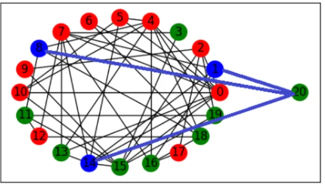
Figure 1.1: The task of community detection: separating groups of vertices into densely connected subgroups (figure from [2])

(8)

Figure 1.2: A social network formed from a single person’s friends, with communities marked in colors; friends from school, friends from college, spouse’s friends, etc. (figure from [3])

Because of its practical interest, a vast number of algorithms have been proposed for community detection. To analyze the performance of these algorithms, improve them, and eventually specifyoptimal algorithms requires mathematical modeling and probabilistic reasoning. Community detection is therefore of interest from a theoretical standpoint, and is a topic of research in both theoretical computer science as well as statistics. The recent review by Moore [4] explains the different viewpoints adopted by different fields. In this work, we adopt an approach that is more popular in the statistics community, which is to study random graph models with planted communities.

1.1 Random graph models

There are two advantages of adopting a random graph model. First, the model specifies the ground truth community structure, which allows us to evaluate the performance of any algorithm in terms of the number of ver-tices that were correctly classified. (In contrast, the min-bisection formula-tion does not lead to this natural error metric.) Such data is typically not available for practical data sets. Second, if one is able to show that an

(9)

al-gorithm achieves a certain performance with high probability (w.h.p.), then that characterizes the algorithm’s performance for a large number of graphs (the typical graphs of the model). This is another desirable property, that gives some performance guarantee on unseen graphs.

The described advantages also come with its set of disadvantages. An algorithm that is shown to be optimal for a certain random graph model may not work well for a graph generated by a different model. In practice, there is no concrete way to determine whether a given graph was generated according to a random graph model or not. There are two ways to tackle this problem: Develop algorithms that arerobust to variations in the model, or study random graph models that are more realistic.

1.1.1 Stochastic block model

By far, the most popular (as well as the simplest) random graph model with planted communities is the stochastic block model (SBM). To generate a graph with two equal-sized communities, one begins with a set of n vertices, and randomly assigns a label ` P t1,2u to every vertex. Having assigned the labels, between any two pairs, an edge is placed with probability pif the two vertices have the same label, and probability q if the vertices have different labels. Usually, we choose p ą q to reflect the fact that entities (people) in the same community are more likely to be connected/linked than those in different communities. A description of the general SBM with any number of communities of possibly different sizes is given in [2]. Given the model, one can generate graphs that have an inherent community structure in them. The task of community detection is to recover the labels from the graph.

The SBM has been analyzed extensively in the literature. Many different algorithms have been proposed, many of which have theoretical guarantees of exactly recovering the communities with high probability for large graphs (e.g., [5], [6]). We review some of these algorithms in Section 1.2.

1.1.2 Preferential attachment graphs

The preferential attachment (PA) random graph model was proposed by Barabasi and Albert in [7] as a more realistic model of real-world networks

(10)

than the Erdos-Renyi model. It describes a random graph that grows with time, as new vertices are added sequentially. At every stage, the new ver-tex chooses a fixed number of neighbors to attach to, within the existing graph (say m). A probability distribution over the vertices is constructed such that the probability of choosing any vertex is proportional to its de-gree. The neighbors are then chosen by sampling with replacement from this distribution m times.

A striking feature of this model is that the graphs have a heavy-tailed degree sequence (in the asymptotic limit). This feature is absent in the Erdos-Renyi model. Loosely speaking, this means that there exist a few vertices whose degree is much larger than the average degree. Such a feature is indeed exhibited in real-world networks such as the web, or in citation networks/social networks. This can be intuitively understood as a fallout of the rich-get-richer phenomenon in the model; vertices that have a high degree at a certain instance are more likely to attract newer vertices than others, and hence their degree is likely to grow even further. This property was first proven rigorously in [8], and is also explained in detail in the book by Van Der Hofstad [9].

1.1.3 Preferential attachment graphs with planted

communities

Much like an Erdos-Renyi graph, the SBM does not have a heavy-tailed degree distribution. In order to develop community detection algorithms that are likely to succeed in real-world networks, it is necessary to study models that have more realistic features. With this aim, we study a model that incorporates community structure within PA graphs, in much the same way as the SBM incorporates communities within Erdos-Renyi graphs. Such a model was first proposed by Jordan in [10], in the context of geometric random graphs. The problem of community detection was not studied in this paper. This is the problem that we study in this thesis.

(11)

1.2 Algorithms for community detection

In this section, we briefly describe a few algorithms that have been proven to work well for community detection in the SBM.

1.2.1 Semi-definite programming

Given a graph generated according to a particular model, the task of finding the labels of the vertices (communities) is an inference problem. The edges (i.e., the graph) is the observed data, and the labels are the unknown pa-rameters, with known prior distribution. In such a scenario, to minimize the probability of error, the best technique is to use the MAP estimator. For any problem, finding the MAP estimator is an optimization problem. For the case of two equal-sized communities, the MAP estimator is the same as finding the minimum bisection of the graph (to partition the vertices into two equal sets such that the number of edges across the sets is minimized). This is well known to be an NP-hard problem. However, it is possible to re-write the problem as a real-valued optimization problem, and then relax certain constraints so as to make it a semi-definite program. Semi-definite programs can be solved in polynomial time. Hajek et al. [5] show that the convex relaxation is tight, and gives exact recovery whenever it is statistically possible.

1.2.2 Spectral methods

The key idea behind spectral methods (for the SBM) is that the expected value of the adjacency matrix of the graph has a low-rank structure, and whose principal components give information about the communities. The expected adjacency matrix is thus the signal of interest. Theactual adjacency matrix is treated as a perturbed version of its expected value. In other words, the true adjacency matrix is the sum of its expected value and a noisy matrix. Loosely speaking, if the noise levels are not too high, the eigenvectors of the perturbed matrix should be close to the eigenvectors of the clean signal, and should thus contain sufficient information about the communities. See [11] as an example of work done along this direction.

(12)

1.2.3 Belief propagation

Belief propagation is a general technique/algorithm to solve inference prob-lems, especially when there are many latent random variables involved. The algorithm is best known in the context of probabilistic graphical models, where random variables are denoted by edges of a “factor graph”, and de-pendencies between them are represented via edges. The algorithm takes advantage of the conditional independence between the random variables, in order to compute the MAP estimator efficiently. The algorithm is guar-anteed to converge to the best estimator if the underlying graph is a tree. In the context of community detection, the given graph itself captures the underlying dependencies in the following manner: the label of one vertex in-fluences (and is influenced by) the number of neighbors it has and the labels of its neighbors, but is conditionally independent of any other vertex label given the labels of its neighbors. Belief propagation algorithms can also be theoretically analyzed, as shown in [12].

(13)

CHAPTER 2 THE RANDOM GRAPH MODEL

We begin this chapter by describing the generative random graph model that we study: preferential attachment graphs with planted communities. This model was first proposed by Jordan in [10]. We first describe the model in the most general setting, where it may include any finite number of com-munities, possible of unequal size. We then describe the parameters for two special cases that are most studied in the literature; that of two equal-sized communities and that of a single community with outliers. Having described the model, we present a fundamental property about the model that greatly simplifies subsequent analysis. This result is also from the paper by Jordan [10]. Finally, we describe and analyze the “degree-growth process”, which serves as a tool for community detection as well as to describe the degree sequence of the graph.

2.1 Model description

The random graph model that we study describes the growth of a labeled, directed graph with time. Equivalently, the model describes a sequence of directed graphstGt:t PNuand labels t`t:tPNu. Gt`1 is built by adding a new vertex and a few connecting edges to Gt, in much the same manner as

in the original preferential attachment graph. The only difference is in the manner in which the neighbors of the new vertex are chosen. To describe the evolution of this process more precisely, we need the following parameters:

• r ě1: number of possible labels; labels are selected from rrs

• ρ = pρ1, . . . , ρrq: probability vector for selection of labels of added

vertices

(14)

• β P Rrˆr: matrix of strictly positive affinities for vertices of different

labels; βuv is the affinity of a new vertex with label u to an existing

vertex of label v

• t0 ě1: initial time

• Gt0 “ pVt0, Et0q: initial directed graph withVt0 “ rt0sand mt0 directed

edges

• T ět0: final time

Given the labeled graph Gt, the graph Gt`1 is constructed as follows: 1. The vertex t`1 is added and its label `t`1 is randomly selected from

rrs using distributionρ, independently of Gt.

2. Themvertices inVt“ rtsare selected using sampling with replacement

according to a distributionftonrts. The distributionftis proportional

to the degree of the verticesand is weighted based on the affinity matrix

β (this is the key difference from the standard preferential attachment model).

3. The m directed edges are added, with tails at vertex t`1 and with heads attached to the vertices chosen in step 2.

Figures 2.1-2.3 provide an illustration for these three steps.

In this model, vertices are referred to by their time of arrival. Let τ be some vertex in the graph, and consider a time point t ě τ. Let the degree of τ at time t be denoted by Y_tτ. When vertex t `1 arrives, each edge from t`1 attaches to vertex τ with probability proportional to Y_tτβ`t`1`τ.

Therefore, the number of edges from vertex t`1 to τ is a random variable with distribution: L`# edges between pt`1, τq|Gt, `r1,t`1s ˘ “ Binom ˆ m, β`t`1`τY τ t ř τ1β`t`1`τ1Y τ1 t ˙ (2.1) L stands for probability law or probability distribution.

Remark 1. For concreteness, one may assume that the initial graph has one vertex with m self-loops, and its label is chosen randomly with distribution ρ. However, all the asymptotic results are independent of the initial graph.

(15)

Figure 2.1: New vertex arrives

Figure 2.2: Label is randomly assigned to the new vertex

Figure 2.3: New vertex attaches to existing vertices using preferential attachment rule

(16)

A graph with two equal-sized communities can be created by choosing the parameters r “ 2, ρ “ p0.5,0.5q, β “ « b 1 1 b ff

, where b ą1. The parameter

m dictates the sparsity of the graph, and can be an arbitrary finite number (usually chosen to be much smaller than the size of the graph, T).

A graph with a single community with outliers can be created by choosing the parameters r “ 2, β “

«

b 1

1 1 ff

, where b ą 1. The parameter ρ dictates the size of the community. As above, the parameter m dictates the sparsity of the graph.

Having described the model, we move on to studying its characteristics. As mentioned earlier, the above model has features of both the PA model and the SBM. Thus, two properties that we expect in the model are:

1. a heavy-tailed degree sequence, like the PA model

2. existence of algorithms that (at least) partially recover the communi-ties, as in the SBM

The heavy-tailed degree sequence property was proven in [10]; we only quote the result here and give empirical evidence in Section 2.5. This thesis focuses on the community detection aspect. We develop a message passing algorithm for community detection, and demonstrate empirically that it per-forms partial recovery. The algorithm and its derivation is given in Chapter 4, and the simulation results are given in Chapter 5. Before we proceed, however, we discuss a few basic results in the rest of this chapter that prove useful for further analysis.

2.2 Half-edges and their convergence

To analyze preferential attachment graphs, it is helpful to have a notion of a “half-edge” (see, e.g., [8]). In any graph, each edge is composed of two half-edges, one attached to each vertex the edge is incident on. Therefore, the degree of a vertex is the number of half-edges attached to it. In the PA model, the affinity to larger degree vertices can be viewed in terms of a tendency of an existing half-edge to attract newer half-edges. At every epoch, there are m new half-edges. Every incoming half-edge has an equal affinity

(17)

toward existing half-edges. In other words, it chooses a partner half-edge uniformly at random (with probability 1{2mt).

In preferential attachment graphs with labels, each half-edge inherits the label of the vertex it is incident upon. Given the labels, the affinity between half-edges is no longer uniform; they are weighted by a factor βuv, where

u, v are the labels of the new and existing half-edges respectively (hence β

is called the affinity matrix). Moreover, the exact probability of attachment depends upon how many half-edges of each type there are at that point of time, which makes analysis difficult.

Suppose the labels of all vertices ofGt are known. Let the fraction of

half-edges with label v inGt be ηv,t. The probability that an incoming half-edge

with label u attaches to an existing half-edge with labelv is θu,v,t

mt , where θu,v,t“ βuv 2ř v1βuv1η_v1_,t (2.2) This follows from the following analysis:

ÿ τ1_Pr_t_s βu`1 τY τ1 t “ ÿ v1_Pr_r_s βuv1 ¨ ˝ ÿ τ1_Pr_t_s Y_tτ11`_τ1“v1 ˛ ‚« p2mtq ÿ v1_Pr_r_s βuv1η_v1

Although the above expression is complex, it simplifies significantly in the asymptotic limit, due to the following result, originally given in [10]:

Proposition 1 (convergence of fraction of half-edges).

ηv,t a.s.

ÝÝÑηv˚ @ v P rrs

where η˚

” tη˚

vuvPrrs is a probability vector that is determined based on the

parameters ρ, β. (The exact characterization of η˚

v is given in [13].)

As an immediate corollary, we have that for large t, the probability that an incoming half-edge with label uattaches to an existing half-edge of label

v is approximately θu,v mt, where θu,v fi βu,v 2ř_v1_Pr_r_sβu,v1η˚_v (2.3) and is independent of the labels of the other vertices. This setting is now

(18)

very similar to the PA model, with θu,v replacing 1{2. The parameters θu,v

in this model play a similar role to the parameters pu,v in the SBM.

A rigorous proof of Proposition 1 is given by Jordan [10]. Here, we just give the outline of the proof. It is shown that the vectortηv,tuvPrrsvaries with time

according to a stochastic approximation scheme with decreasing step-sizes. The stochastic approximation scheme is viewed as a noisy discretization of an appropriate ordinary differential equation (ODE) [14]. It is shown in [10] that the underlying differential equation has a unique, globally asymptot-ically stable (GAS) equilibrium, by constructing an appropriate Lyapunov function. The convergence of the underlying ODE implies convergence of the stochastic approximation recursion [14].

2.3 The degree growth process

In this section, we study the degree growth process, i.e., the growth of the degree of a fixed vertex in the graph with time. Due to the time-evolutionary nature of the model, the degree is best described as a random process, rather than a random variable. Obtaining the distribution (or probabilistic descrip-tion) of the degree of a vertex allows us to establish both the properties mentioned above:

1. Degree sequence: Characterizing the degree sequence of graphGT is

equivalent to calculating the probability of a vertex picked uniformly at random amongrTshas degree greater thank, for each k. To get this figure, it is useful to know the probability of the degree of each vertex

τ being greater than k. Studying the degree-growth process gives us this probability.

2. Community detection: If the time of arrival of a vertex is known, then the degree of a vertex is simply dependent upon its label. If the distributions of the degree for different labels are well separated, one can infer the labels by observing the degree. This is true for the model of a single community with outliers (but not the case of two equal-sized communities). Knowing the exact distribution of the degree allows us to formulate a hypothesis testing problem.

(19)

Having motivated the study of the degree-growth process, we now define it formally.

Definition 1 (The degree growth process). Given a vertex τ withτ ět0`1, consider the process pYt:těτq, where Yt is the degree of vertex τ at timet.

Thus Yτ “m. The conditional distribution (i.e. probability law) of Yt`1´Yt

given pYt, ηt, `τ “v, `t`1 “uq is given by:

LpYt`1´Yt|Yt, ηt, `τ “v, `t`1 “uq “ binom ˆ m,θu,v,tYt mt ˙ (2.4) where θu,v,t is given by (2.2). It follows that, given pYt, ηt, `τ “vq, the

con-ditional distribution of Yt`1 ´Yt is a mixture of binomial distributions with

selection probability distribution ρ: LpYt`1´Yt|Yt, ηt, `τ “vq “ ÿ uPrrs ρubinom ˆ m,θu,v,tYt mt ˙ (2.5)

The above probability law essentially follows by rewriting (2.1) using the notion of half-edges introduced above:

L`# edges between pt`1, τq|Gt, `r1,t`1s ˘ “binom ˆ m,θu,v,tYt mt ˙ (2.6) From Proposition 1, we see that in the asymptotic limit, the parameters

θu,v,t converge toθu,v. Moreover, for large t, the quantity θ_mtu,v is really small.

A binomial random variable with a small p parameter takes values either 0 or 1 with high probability, and can thus be approximated by a Bernoulli random variable of the same mean. With these considerations, we see that:

LpYt`1´Yt|Yt, ηt, `τ “vq “ ÿ uPrrs ρubinom ˆ m,θu,v,tYt mt ˙ (2.7) « ÿ uPrrs ρubinom ˆ m,θu,vYt mt ˙ « ÿ uPrrs ρuBer ˆ θu,v dτptq t ˙ “Ber ˆ θv dτptq t ˙ (2.8) whereθv fi ř

(20)

probability law in the asymptotic regime.

In Proposition 3 of [13], the above approximation is made more precise. This is stated in terms of the total variation distance between the actual degree-growth process and an idealized version of it going to zero in the asymptotic limit. We first define a random process Yr that is an idealized variation ofY obtained by replacingηtby the constant vectorη˚ and allowing

jumps of size one only.

Definition 2. The process Yr has parameters τ, m, and ϑ, where τ is the initial time, m is the initial state, and ϑ ą 0 is a rate parameter. The process Yr is a time-inhomogeneous Markov process with initial value m. Yr is defined as follows: for t ěτ and y such that ϑy_t ď1, we require

pYr_t_`₁´Yr_t|Yr_t“yq d. “Ber ˆ ϑy t ˙ (2.9) We have the following coupling result.

Proposition 2. Suppose τ, T Ñ 8 such that T ą τ and T{τ is bounded. Fix v P rrs. Then

dT VppYrτ,Ts|`τ “vq,Yr_r_τ,T_spθ_vqq Ñ0 (2.10) From Proposition 2, we infer that the degree growth process is essentially a time-inhomogeneous Markov process in the asymptotic limit. It is interesting to note that the degree growth process depends on m only via its initial condition. The state may either increase by 1, or stay the same at any point of time. The parameter θv gives us the rate of growth or the “jump rate” of

this process. The larger this parameter, the larger is the rate at which the degree of vertex τ grows. This property is useful for community detection, as explained in Section 1.2.

Remark 2. The line of arguments leading to (2.8) can also incorporate par-tial or complete information about other vertex labels. Suppose, from some other considerations, we know that the distribution of `t`1 is ρr. Then this distribution may be used in place of ρ in (2.8). We do not use this property here, but it is used in formulating the message passing algorithm later.

(21)

2.4 The

Z

-process

The process Yr can be thought of a discrete time birth process with activa-tion time τ and birth probability at a time t proportional to the number of individuals. However, the birth probability (or birth rate) per individual,

θu,v

t , has a factor

1

t, which tends to decrease the birth rate per individual.

This makes the process difficult to analyze. By a simple time-scaling, we can obtain a process with constant birth rate. The scaling involves considering the process pYes : s ě 0q. The intuition behind the scaling is the following:

the graph of the function logt has slope 1{t. By scaling the horizontal axis exponentially, we obtain the function logpetq “t, which has a constant slope 1.

Definition 3(Z-process). The processZ “ pZs:s ě0qis a continuous time

pure birth Markov process with initial stateZ0 “m and birth rateϑk in state

k, for some ϑą0. The process Z represents the total number of individuals in a continuous time branching process beginning withmindividuals activated at time 0, such that each individual spawns another at rate ϑ.

Definition 4. Let Yq_t“Z_ln_p_t_{_τ_q for integers těτ

The following proposition, proven in [13], shows thatYr andYq are asymp-totically equivalent in the sense of total variation distance.

Proposition 3. For any ϑą0,

dT V ´ r Yrτ,Tspϑq,Yq_r_τ,T_spϑq ¯ Ñ0 (2.11)

Propositions 2 and 3 allow us to map many properties about theZ-process to the degree-growth process. We illustrate this by calculating the distribu-tion of the degree of any vertex τ at time T.

We first establish the following useful fact about theZ-process.

Proposition 4. For fixed s, Zs has the negative binomial distribution

negbinompm,e´sϑ_q. _{In other words, its marginal probability distribution}

pπnps, ϑ, mq:nPNq is given by πnps, ϑ, mq “ ˆ n´1 m´1 ˙ e´mϑs_p1 ´e´ϑs qn´m for něm (2.12)

(22)

In particular, taking m “ 1 shows πps, ϑ,1q is the geometric distribution with parameter e´ϑs_{, and hence, mean e}ϑs_.

Proof. We prove the result only form“1. Formě2,the processZ has the same distribution as the sum of m independent copies ofZ with m“1. The negative binomial distribution is also the sum of m independent geometric distributions, from which the result follows.

We shall prove thatπips, ϑ,1q “ e´ϑsp1´e´ϑsqi´1 by induction oni.

Induction base: From Definition 3, we see that the time stayed in stateiis a random variable with distribution Exppλiq. Therefore, π1ps, ϑ,1q “ e´ϑs_,

since it is the probability that the system was in state 1 for time more than

s.

Induction step: Forią1,πips, ϑ,1qincreases by the influx from statei´1

and decreases by the outflux from state i.

dπips, ϑ,1q ds “ ´iϑπips, ϑ,1q ` pi´1qϑπi´1ps, ϑ,1q ; πip0q “0 πips, ϑ,1q “ żs 0 e´iϑps´τqpi´1qϑπi´1pτ, ϑ,1qdτ

By the induction hypothesis, πi´1ps, ϑ,1q “e´ϑsp1´e´ϑsqi´2. Performing a change of variables τ Ñeϑτ ´1 in the integral above gives us the necessary expression for πiptq.

We now have the following corollary from Proposition 4: Corollary 1. For T ąτ ąą1, LpYTτ|`τ “vq «NegBinom

`

m,pT{τqθv˘

.

2.5 Asymptotic degree distribution

A second limit result we restate from [10] concerns the empirical degree distribution for the vertices with a given label. For v P rrs and integers

n ěm and T,let:

• Hv_p_T_q _{denote the number of vertices with label}_v _in _G T

• Nv

npTqdenote the number of vertices with labelv and with degreenin

(23)

• Pv npTq “

Nv npTq

Hv_p_T_q denote the fraction of vertices with label v that have

degree n in GT

Proposition 5 (Limiting empirical degree seq. for a given label [10]). Let

n ěm and v P rrs be fixed. Then limTÑ8PnvpTq “ pnpθv, mq almost surely,

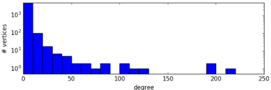
where pnpθ, mq “ Γ`1_θ `m˘Γpnq θΓpmqΓ`n` 1_θ `1˘ — « Γ`1_θ `m˘ θΓpmq ff 1 n1θ`1 (2.13) Proposition 5 is illustrated by plotting the degree distribution of a graph with the structure of a single community with outliers. To illustrate some interesting features, we plot the degree distribution of vertices in the commu-nity and outside separately, in Figures 2.4 and 2.5 respectively. The param-eters chosen are m “ 1, b “4, T “10,000, ρ “ p0.5,0.5q. In such a setting, the average degree of the graph is 2. As expected, we do see that there are vertices of both types with degrees much higher than the average degree. Further, we also see that vertices within the community have a higher degree on average than vertices outside the community. It is precisely this property that is exploited in the degree thresholding algorithm described in Chapter 3.

(24)

Figure 2.4: Degree distribution within community

(25)

CHAPTER 3 COMMUNITY DETECTION

ALGORITHMS-BINARY HYPOTHESIS

TESTING

In this chapter, we formulate the problem of community detection as a statis-tical inference problem. The labels on the vertices are the hidden variables, and the observed data is the graph, from which the labels must be inferred. Although, in principle, one can write down the likelihood of observing a given graph for every possible sequence of vertex labels, t`tuTt“1 this expression is immensely complex. It is thus infeasible to optimize over the set of possible vertex labels and find the maximum aposteriori probability (MAP) estima-tor. We thus settle for other estimators that are easier to compute. These estimators are shown to be MAP estimators for certain simpler problems.

One simplification is to decouple the inference problem for different ver-tices. This simplifies the problem immensely, since instead of optimizing over rT _{possible choices, one only has to optimize over} _r _{choices. A second}

simplifying technique is to perform the inference based only on observing a small neighborhood of the vertex, instead of the whole graph. This allows us to have a simple expression for the likelihood of the observation, conditioned on the label.

For concreteness, consider the model of a single community with outliers, where θ1 ą θ2 (the label 1 indicates that the vertex is in the community). Consider any vertex τ s.t. 1ăăτ ăT with `τ “v. The number of children

of τ has distribution „ NegBinom`m,pT{τqθv˘ _{as seen from Corollary 1.}

Thus, observing the number of children gives some information about the label v; the larger the number of children, the more likely it is that the vertex belongs to the community.

In fact, using the results from Chapter 2, we can compute the likelihood of observing the entire degree-growth process of any vertex τ. This allows us to calculate the MAP estimator of the vertex label based on additional information of which vertices attached to τ. This idea is presented in more detail in the rest of this chapter.

(26)

The algorithms presented in this chapter can be used, in principle, to perform community detection for any set of parameters ρ, β, as long as θv ‰

θv1 for v ‰ v1. However, for brevity, we focus only on the case of a single

community with outliers. Note that these algorithms cannot be used to identify labels in a graph with equal-sized communities.

To comply with standard notations of binary hypothesis testing, we slightly change our notation:

• `τ “1: Vertex is in the community

• `τ “0: Vertex is an outlier

3.1 Binary hypothesis testing

Let 1 ăă τ ă T be integers. Consider the problem of estimating `τ given

observation of a random object O. For instance, the object could be the degree of vertex τ in GT, or it could be the set of children of τ in GT, or it

could be the entire graph. We have two hypotheses about the label `τ:

H1 :`τ “1

H0 :`τ “0

The prior probabilities are π1 “ ρ and π0 “ 1´ρ respectively. We seek to calculate the MAP estimator, which is a decision rule that minimize the average error probability, pe fi π1pe,1 `π0pe,0, where pe,v is the conditional

probability of error given Hv is true.

For binary hypothesis testing, the MAP estimator can be expressed in terms of thresholding either the log-belief ratio ξ or the log-likelihood ratio Λ: p τM AP “1tξą0u“1tΛąlnpπ0{π1qu ξ filnPtH1|Ou PtH0|Ou Λfiln ppO|H1q ppO|H0q

Algorithm C The first recovery algorithm we describe, Algorithm C (“C” for “children”), is to let O denote the set of children, Bτ “ tt1, . . . , tnu,

(27)

tt1, . . . , tnuwithτ`1ďt1 ă ¨ ¨ ¨ ătn ďT, lety_rB_τ,Tτ _sdenote the corresponding

degree evolution sample path: yBτ

t “m` |BτX rτ, ts| forτ ďtďT.

Proposition 2 allows us to approximate the probability of observing a sam-ple path of Y with the probability of observing the same sample path of Yr.

PpBτ “ tt1, . . . , tnuq “PpYrτ,Ts “yrBτ,Tτ sq «PpYr_r_τ,T_s “y_rB_τ,Tτ _sq “ ź tPrτ`1,TszBτ ˆ 1´y Bτ t´1θv˚ t´1 ˙ ź tPBτ yBτ t´1θ˚v t´1 so the log-likelihood ratio for observation Yr_r_τ,T_s “yBτ

rτ,Ts is ΛC “nlnθ ˚ 1 θ˚ 0 ` ÿ tPrτ`1,TszBτ ln ˆ 1´y Bτ t´1θ1 t´1 ˙ ´ln ˆ 1´y Bτ t´1θ0 t´1 ˙

Algorithm C for estimating `v is to perform the likelihood ratio test using

ΛC_. _{Using the approximation ln}

p1`sq “ s and approximating the sum by an integral, we find ΛC «nlnθ1 θ0 ´ pθ1´θ0q żT τ yBτ t t dt “nlnθ1 θ0 ´ pθ1´θ0q ˜ mlnpT{τq ` ÿ tPBτ lnpT{tq ¸ (3.1) Algorithm C is similar to performing hypothesis testing based on O “

Zr0,¯ss,where ¯s“lnpT{τq. LetfZCpρ, θ1, θ0, m,s¯q denote the resulting average error probability pe. This quantity is estimated Section 3.2.

Algorithm DT The second recovery algorithm we describe, Algorithm DT (“DT” for “degree thresholding”), is to let O denote the number of children of vertex τ inGT. Equivalently, O denotes the observation of YT.

Here too, using Proposition 3, we approximate the distribution of YT by

that of Yq_T, which has the negbinom `

m,pτ{Tqθv˘ _{distribution under} _H

v for

(28)

is n, is ΛDT “ ´mpθ1´θ0qlnpT{τq ` pn´mqln ˆ 1´ pτ{Tqθ1 1´ pτ{Tqθ0 ˙

Algorithm DT for estimating `v is to perform the likelihood ratio test using

ΛDT, or in other words, the MAP decision rule based on O “ YT. This is

similar to performing hypothesis testing based onO “Z¯s,where ¯s“lnpT{τq

(becauseYq_T “Z_¯_s). Letf_ZDTpρ, θ₁, θ₀, m,¯sqdenote the resulting average error probability pe. It is clear that we expectfZDT ěfZC, as Algorithm C is based

on more information.

3.2 Hypothesis testing for

Z

We consider here the binary hypothesis testing problem based on observation of Z_r0,lnpT{τqs such that under Hv it has rate parameterϑ “θv for v P t0,1u.

To this end, we derive the likelihood ratio.

Suppose ts1, . . . , snu Ă p0,s¯s such that 0ă s1 ă ¨ ¨ ¨ ăsn and ¯s“ lnT{τ.

Since the inter-jump periods are independent (exponential) random variables, the likelihood of s1, . . . , sn being the jump times duringr0,¯ss under

hypoth-esisHv, is the product of the likelihoods of the observed inter-jump periods,

with an additional factor of the likelihood of not seeing a jump in the last interval: ˜_n_´₁ ź i“0 θvpm`iqe´θvpm`iqpsi`1´siq ¸ e´θvpn`mqps¯´snq

Thus, the log-likelihood ratio for observing this is (letting s0 “0): ΛZ “nlnθ1 θ0 ´ pθ1´θ0q ˜ ms¯` n ÿ i“1 p¯s´siq ¸ (3.2) (With si “lnpti{τq, (3.2) is the same as (3.1), although in (3.1) the variables

ti are supposed to be integer valued.) Let As¯ fi pms¯` řn

i“1p¯s´siqq. Note

that A¯s is the area under the trajectory of Zr0,s¯s. Moreover, n`m is the

value of Z¯s. So the log-likelihood ratio is given by

ΛZ “ pZ¯s´mqln

θ1

θ0

(29)

which is a linear combination of Z¯s´mandAs¯.Thus, the MAP decision rule has a simple form. LetfC

Zpρ, θ1, θ0, m,¯sqdenote the average error probability

pe for the M AP decision rule based on observation of Zr0,¯ss.

There is apparently no closed-form expression for the distribution of ΛZ_,

so computation offC

Zpρ, θ1, θ0, m,s¯qrequires Monte Carlo simulation or some other numerical method. A closed-form expression for the moment generating function of ΛZ is given in the following proposition, which can be used to bound the probability of error. The proof of Proposition 6 is given in [13]. Proposition 6. The joint moment generating function of Zs andAs is given

as follows, where _Eλ,mr¨s denotes expectation assuming the parameters of Z

are λ, m : ψλ,mpu, v, sqfiEλ,m “ euZs`vAs‰ “ ˜ epv´λqsù 1` _vλe_ú_λp1épv´λqs_q ¸m (3.4) Proposition 6 can be used to bound pe as follows. By a standard result in

the theory of binary hypothesis testing, the probability of error for the MAP decision rule is bounded by

π1π0ρ2B ďpe ď

?

π1π0ρB (3.5)

where the Bhattacharyya coefficient (or Hellinger integral) ρB is defined by

ρB “E

“ eΛ{2ˇ

ˇH₀ ‰

,andπ1andπ0are the prior probabilities on the hypotheses. The proposition with λ“θ0, u“ 1₂lnpθ1{θ0q, v“ ´θ1´₂θ0, and s “s¯yields

ρB,C “Eλ,m “ eupZs´mq`vAs‰ “ψλ,mpu, v, sqe´mu “ ˜ e´pθ1`θ0q¯s{2 1´2 ? θ1θ0 θ1`θ0 p1´e ´pθ1`θ0qs¯{2_q ¸m

Here we wrote ρB,C to denote it as the Bhattacharyya coefficient for

Algo-rithm C (for the largeT limit). Using this expression in (3.5) provides upper and lower bounds on pe“fZCpρ, θ1, θ0, m,s¯q.

For the sake of comparison, we note that the Bhattacharyya coefficient for the hypothesis testing problem based on Yq_T alone, i.e. Algorithm DT, is

(30)

easily found to be ρB,DT “ ˜ e´pθ1`θ0q¯s{2 1áp1é´θ1s¯qp1_é´θ0s¯_q ¸m

(31)

CHAPTER 4 MESSAGE PASSING

In this chapter, we describe how Algorithm C (the MAP rule given children) can be extended to a message passing algorithm. The message passing algo-rithm performs better than Algoalgo-rithm C in recovering the labels of a graph with a single community with outliers, as each vertex takes into account more information than just its set of children. Further, message passing allows us to recover planted communities in graphs with equal-sized communities, which is impossible via Algorithms C and DT.

4.1 Overview

In Algorithm C, it was assumed that there was no prior information about the labels of any of the vertices. Here, information about a vertex label means a distribution of the vertex label that is not the prior distribution (this includes knowing the vertex label exactly). Message passing extends Algorithm C to take into account information about the children’s labels. In addition, it takes into account any information about the parents’ labels. Intuitively, having more information about one’s neighbors’ labels allows one to compute a better estimate of one’s own label, as they are correlated.

In Chapter 3, we showed that Algorithm C gives some information about a vertex’s label. If this information is passed on to the vertex’s parent (as a message), the parent can form a better estimate of its own label. Messages from one vertex to another are posterior distributions of the sender’s vertex label (or equivalent information). In effect, the parent vertex observes the graph up to a depth of two. Upon iterating, each vertex sees a larger portion of the graph at every step, ultimately observing the whole graph. In the rest of this chapter, we make the above notions precise. We discuss what the messages mean, how they are computed and sent from one vertex to the

(32)

other, and make clear why indeed the extra information is useful for better inference.

We describe the algorithm for the case of two possible labels for a general 2ˆ2 matrix β with positive entries, and fixed m ě 1. The algorithm can be extended for the case of more than two communities, as shown in [13]. For binary valued random variables, distributions can be inferred from log-likelihood ratios, which is a compact representation (a scalar instead of a two-dimensional vector). Thus, all messages are represented here as log-likelihood ratios.

In general, a message passing algorithm on any graph is an iterative algo-rithm where vertices in the graph send “messages” to their neighbors based on messages that they receive in the previous iteration. Specific to the appli-cation at hand, messages are ascribed a certain meaning, and are computed accordingly. Message passing algorithms are generally used to solve infer-ence problems in a factor graph (or more generally, a probabilistic graphical model) (see, e.g., [15]). A factor graph is a graphical representation of the joint distribution of multiple random variables, that takes into account the dependence (and conditional independence) conditions among the random variables. The advantage of this representation is that the marginal distri-bution (or marginal conditional distridistri-bution) of any random variable can be computed efficiently via a particular form of message passing called belief propagation. In belief propagation, the messages in every iteration can be thought of as a particular distribution.

For community detection, the message passing algorithm is similar to belief propagation, except for the fact that one does not construct a fac-tor graph. The algorithm is run on the given graph itself, as the depen-dence/independence conditions are well represented by the given graph. In the rest of this section, we state and then derive a principled message passing algorithm for inferring the label of each vertex, given the graph. Throughout the remainder of this section, let pV, Eq be a fixed instance of the random graph,pVT, ETq,with two communities and known parametersm, β, ρ, to, Gto,

and T. The message passing algorithm is run on this graph, with the aim of calculating Λτ for 1ďτ ďT, where for each τ, Λτ is a log-likelihood ratio:

Λτ filnP

tET “E|`τ “1u

PtET “E|`τ “0u

(33)

Then we can calculate the maximum likelihood (ML) and maximum a pos-teriori probability (MAP) estimators of the label of a vertex τ as prescribed in Chapter 3. This estimator gives us the smallest probability of error in inferring each vertex.

Remark 3. Note that this does not give us an estimator that gives us the smallest error of getting the entire set of vertices correct. See [2] for a detailed discussion on the best estimators for exact recovery versus partial recovery.

4.2 Algorithm

A complete specification of a message passing algorithm includes specification of the following elements:

1. initial messages

2. mappings from messages received at a vertex to messages sent by the vertex

3. timing of message passing and termination criterion

4. mappings from messages received at a vertex to the output log-likelihood vector of the vertex

In this section, we specify the equations for elements (1), (2), and (4). A discussion on element (3) is given in the chapter on simulations (Chapter 5). To specify these equations, we need the following notation. Given verticesτ

and τ0, we say τ is a child ofτ0, andτ0 is a parent ofτ, ifτ ěmaxtτ0, tou `1,

and there is an edge from τ toτ0.It is assumed that the known initial graph

Gto is arbitrary, i.e., they are not placed according to particular model. Thus,

for the inference problem at hand, the edges in Gto are not relevant beyond

the degrees that they imply for the vertices in Gto.

LetBτ denote the children of τ inGT and℘τ the parents of τ.So℘τ “ H

if τ ďto and Bτ Ă tto `1, . . . , Tu. Let ντÑτ0 denote a message passed from

(34)

The functions gcp _:

R ÞÑ R and gpc : R ÞÑ R are defined as follows (here

“cp” denotes child to parent, and “pc” denotes parent to child):

gcppνq “ ln ˆ eν_{ρ θ} 1,1 ` p1´ρqθ0,1 eν_{ρ θ} 1,0 ` p1´ρqθ0,0 ˙ ´lnθ1 θ0 for ν PR gpcpµq “ ln ˆ eµρ θ1,1` p1´ρqθ1,0 eµ_{ρ θ} 0,1` p1´ρqθ0,0 ˙ for µPR

where θu,v and θv are defined in Section 2.2.

For convenience, we repeat the expression in (3.1) for the log-likelihood ratio based on observation of children, for any vertex τ:

λC_τ “ |Bτ|lnθ1 θ0 ` pθ1´θ0q ˜ d0pτqlnτ _to T ` ÿ tPBτ ln t T ¸ (4.2) where τ_to “maxtτ, tou and d0pτq is the initial degree of vertex τ, defined

to be the degree of τ in Gto if τ ď to and d0pτq “ m otherwise. This slight

modification from (3.1) takes into account the fact that an initial vertex’s degree growth process starts effectively at time to, and such a vertex can

have arbitrary initial degree, not necessarily m. The message passing equations are given as follows:

ντÑτ0 “λ C τ ` ÿ tPBτ gcppνtÑτq ` ÿ τ1P℘τztτ0u gpcpµτ1Ñτq (4.3) µτ0Ñτ “λ C τ0 ` ÿ tPBτ0ztτu gcppνtÑτq ` ÿ τ1P℘τ0 gpcpµτ1Ñτq ´ln θ1 θ0 (4.4) Λτ “λCτ ` ÿ tPBτ gcppνtÑτq ` ÿ τ0P℘τ gpcpµτ0Ñτq (4.5)

with the initial conditions:

ντÑτ0 “λ C τ µτ0Ñτ “λ C τ0 ´ln θ1 θ0 (4.6) The message passing equations are written as if there are no parallel edges inpV, Eq. While the fraction of edges that are parallel to other edges will be small for large T, they are permitted. The convention used in the message passing algorithm is that Bτ and ℘τ are to be considered as multisets, so that if a vertex appears with some multiplicity in one of those sets, then the corresponding term in the summations will be appearing the corresponding

(35)

number of times. The initial conditions given by (4.15) are chosen to mimic the scenario of Algorithm C, where no messages are received.

Essentially, each vertex assimilates all the incoming messages to form an estimate of its own log-likelihood ratio. It then passes this quantity to all of its neighbors (with a small modification), so that they may use this in-formation in their own likelihood calculations. The modification is to not include information gained from one neighbor in the message being sent to that neighbor. This form of the messages appears naturally in deriving the messages assuming the graph is a tree, and is a useful heuristic even in loopy message passing.

4.3 Derivation

Instead of deriving the message passing algorithms as stated above, we shall state and derive them in a slightly different form. The advantage of this alternative form is that the derivation becomes much more intuitive. The only price we pay is that of additional notation. Following the derivation, we show how the alternate form of the messages is equivalent to the original form presented in equations (4.3) - (4.5).

In what follows, message passing equations are stated and derived for the special case m “ 1, with the initial graph Gto consisting of a single vertex

(i.e. to “1) with a self-loop. In that case, the graphpV, Eqis a tree (ignoring

any self-loops among the initial vertices) so the message passing algorithm is conceptually simpler. Equations (4.3) - (4.5) for any finite m ě 1 are simply taken to have the same form as for m “1 on the grounds that loopy message passing is obtained by using the same equations as for message passing without loops.

A second major difference from the equations given in Section 4.2 is that here, the messages are vectors in _R2_{, rather than scalar quantities. This is} because the earlier set of messages were interpreted as log-likelihood ratios, while here, the messages are simply log-likelihoods.

(36)

4.3.1 Alternate form

Let the notation of Bτ, ℘τ be the same as before. We abuse notation by redefining certain quantities differently than before as follows:

gcppνqpvq “ ln ¨ ˝ ÿ uPrrs eνpuq_ρ u θu,v θv ˛ ‚for ν PRr (4.7) gpcpµqpuq “ ln ¨ ˝ ÿ vPrrs eµpvq_ρ v θu,v θv ˛ ‚for µP_Rr (4.8) λC_τpvq “ |Bτ|lnθv `θv ˜ d0pτqlnτ_to T ` ÿ tPBτ ln t T ¸ (4.9) The new message passing iterative equations are given by

ντÑτ0 “λ C τ ` ÿ tPBτ r νtÑτ (4.10) µτ0Ñτ “λ C τ0` ÿ tPBτ0ztτu r νtÑτ0 `rµτ1Ñτ0 (4.11) r ντÑτ0 “g cp pντÑτ0q (4.12) r µτ0Ñτ “g pc pµτ0Ñτq (4.13) Λτ “λCτ ` ÿ tPBτ r νtÑτ `µrτ0Ñτ (4.14)

with the initial conditions: r ντÑτ0 “0 µrτ0Ñτ “0 (4.15) or equivalently ντÑτ0 “λ C τ µτ0Ñτ “λ C τ0 (4.16)

Note that the above are vector equations; they are to be interpreted as per-forming the same operation component-wise.

The initial conditions are chosen such that the initial value of Λτ “ λCτ.

That is, the first step of message passing is equivalent to performing Algo-rithm C.

(37)

4.3.2 Derivation of alternate form

Conceptually, we view the entire graph as the collection of children sets of different vertices. As before, Bτ denotes the children set ofτ. Bτ is a random quantity, while Bτ “ tt1, . . . , tnu is an event. Let Dτ denote the set of all

descendants of τ in the given graph. This includes the observation that Bτ “ tt1, . . . , tnu, Bt1 “ tt1,1, . . . , t1,n1u, and so on. The entire graph is thus

represented by D1.

To derive the above recursion, we first define the quantitiesν, µ,ν,_r µ,_r Λ to be appropriate log-likelihoods. Equations (4.10) - (4.14) then follow from the relation among these log-likelihood quantities.

The aim of message passing is to calculate the log-likelihood ratio of each vertex’s label upon observing the whole graph. Thus, we define Λτ as

ΛτpvqfilnPtD1|`τ “vu (4.17)

Using the following identity:

PtD1|`τ “vu “ PtD1zDτ|`τ “vuPtDτ|`τ “vu

“PtD1zDτ|`τ “vuPtBτ|`τ “vu

ź

tPBτ

PtDt|`τ “v,Bτu

and the definitions: r µτ0ÑτpvqfilnPtD1zDτ|`τ “vu (4.18) r νtÑτpvqfilnPtDt|`τ “v,Bτu (4.19) we get Λτ “λCτ ` ÿ tPBτ r νtÑτ`µrτ0Ñτ which is (4.14).

(38)

Plugging this definition into (4.20), we obtain (4.12):

r νtÑτpvq “ ln ¨ ˝ ÿ uPrrs eνtÑτpuqθu,v θv ρu ˛ ‚

From the definition ofνtÑτ, and the following identity:

PtDτ|`τ “vu “PtBτ|`τ “vu ź tPBτ PtDt|`τ “v,Bτu we get (4.10): νtÑτ “λCτ ` ÿ tPBτ r νtÑτ

(39)

We know that PtD1zDτ|`τ “vu “ ÿ v1 PtD1zDτ|`τ “v, `τ0 “v 1 uPt`τ0 “v 1 u “ ÿ v1 PtD1zDτ|`τ “v, `τ0 “v 1 uθv1 θv,v1 θv,v1 θv1 ρv1 “ÿ v1 eµτ₀Ñτpv1_q θ_v,v1 θv1 ρv1 ñrµτ0Ñτpvq “ ln ˜ ÿ v1 eµτ₀Ñτpv1_q ρv1 θv,v1 θv1 ¸ (4.22) In deriving (4.22), we have used the following definition ofµτ0Ñτ:

µτ0Ñτpv 1 qfilnPtD1zDτ|`τ “v, `τ0 “v 1_u_θ v1 θv,v1 (4.23) For this definition to be precise, we need to show that

PtD1zDτ|`τ“v,`τ₀“v1_u_θ v1

θ_v,v1 is independent of v. This is shown below. In parallel,

we derive an expression for µτ0Ñτ.

Combining these into (4.24), we get:

PtD1zDτ0|`τ “v, `τ0 “v 1 u θv1 θv,v1 “eµrτ1Ñτpv1qeλ τ₀ C ź t1_PB_τ 0ztτ0u eνrt1Ñτ₀pv 1_q (4.25)

(40)

Taking the logarithm of (4.25), we get µτ0Ñτ “λ_Cτ0 `µrτ1Ñτ ` ÿ t1_PB_τ₀_zt_τ₀_u r νt1_Ñ_τ₀pv1q

which is (4.11). This completes the derivation of (4.10) - (4.14).

4.3.3 Deriving the original message passing equations

To get the scalar message passing Equations (4.3) - (4.5), we subtract the second component of the vector equations from the first component. This operation indicates that we are working with log-likelihood ratios, instead of log-likelihoods. In particular, the following quantities are now interpreted as: Λτ “lnP tD1|`τ “1u PtD1|`τ “0u (4.26) ντÑτ0 “ln PtDτ|`τ “1u PtDτ|`τ “0u (4.27) µτ0Ñτ “ln PtD1zDτ|`τ “0, `τ0 “1u PtD1zDτ|`τ “0, `τ0 “0u θ1 θ0 θ0,0 θ0,1 (4.28) The quantities µ,r rν are done away with, by substituting (4.12) and (4.13) in (4.10) and (4.11).

Lastly, we sightly modify the definition of µ:

µτ0Ñτ “ln PtD1zDτ|`τ “0, `τ0 “1u PtD1zDτ|`τ “0, `τ0 “0u θ0,0 θ0,1 (4.29) This modification is to let µbe as close as possible to a log-likelihood ratio, without depending upon the label of τ (one could condition on `τ “ 1 as

well). This modification leads to a slight modification of gpc_{, and the adding}

of the term lnθ1

θ0 in (4.4).

4.4 Derivation discussion

The aim of message passing is to calculate Λτ (as defined in (4.1)) for every

(41)

for the case m “ 1. On making some assumptions about the distribution of the graph and about conditional dependencies, the computation becomes more efficient. These assumptions do not hold for any finite-sized graph, but they are good approximations for large graphs.

Conceptually, we view the entire graph as being generated by a set of degree-growth processes. The initial vertex start their degree-growth pro-cesses at time to. Thereafter, every vertex that arrives starts its own

degree-growth process, depending only on its label, but independent of other pro-cesses. This point of view allows us to make some principled assumptions that follow.

• Distribution of Bτ: We assume that the distribution of a children set is according to the law of the process Yq:

PtBτ “ tt1, . . . , tnu|`τ “vu “ n!θvn ˜ τ _to T ˆ ź tPBτ t T ¸θv

Accordingly, given the children set Bτ, the log-likelihood ratio of the vertex label is given by λC_τ.

• Dependence ofBτ on other labels: We assume that the distribution of the children set depends on the labels of only those vertices in the children set, i.e.:

PtBτ “ tt1, . . . , tnu|`τ “v, `τ1 “uu

“ #

PtBτ “ tt1, . . . , tnu|`τ “vuθu,v˚ {θv˚ if τ1 P Bτ

PtBτ “ tt1, . . . , tnu|`τ “vu if τ1 R Bτ

This implies that the posterior distribution of `τ1 given `_τ and Bτ is

given by: Pt`τ1 “u|`_τ “v,Bτu “ PtB τ|`τ “v, `τ1 “uu_Pt`_τ1 “u|`_τ “vu PtBτ|`τ “vu “ # _θ uvρu θv if τ 1 _{P B}_τ ρu if τ1 R Bτ

• Dependence of one children set on another: Given the labels of two vertices τ1, τ2, the distribution of Bτ1 is independent of Bτ2.

(42)

However, if one (or both) of the labels are not known, Bτ1 may convey information on Bτ2 (and vice versa). The exact dependence is seen via an appropriate use of Bayes’ rule and the two points given above.

(43)

CHAPTER 5 SIMULATIONS

In this chapter, we present numerical results of the algorithms described in Chapters 3 and 4. For graphs with a single community with outliers, we run the following algorithms:

• Degree Thresholding (DT)

• Maximum Likelihood based on children (abbreviated as “Children” or C)

• Message Passing (MP)

For the case of two communities, we present simulation results of message passing alone. In this case, the algorithm requires initialization with the labels of few of the vertices. This aspect is also discussed.

5.1 Single community with outliers

We simulate the case of a single community with outliers with the following parameters: • T = 10,000 • β “ ˜ 4 1 1 1 ¸ • m “5 • ρ“ p0.5,0.5q

The values ofθ for these parameters are: pθ1 “0.61, θ2 “0.37q.

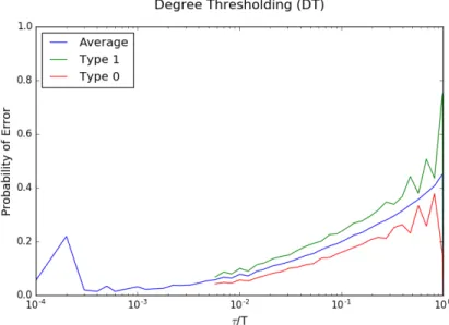
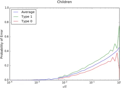
For each of the algorithms DT, C and MP, we display the probability of error in recovering the label of vertexτ,Pepτq, as a function ofτ (see Figures

(44)

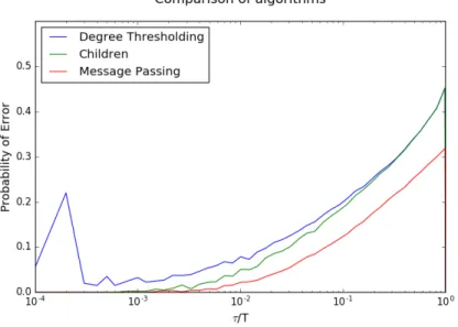
5.1, 5.2 and 5.3 respectively). Each plot is an average over 1000 random graphs. From the analysis of Chapters 3 and 4, we expect that this quantity would depend only on τ{T; hence, we scale the axis accordingly. We also plot the probability of error of type 1 and type 0 (as discussed in Chapter 3) for each of the algorithms. Finally, we compare these three algorithms in Figure 5.4, from which we see two trends:

• Algorithm C performs significantly better than Algorithm DT for ver-tices that arrived earlierτ{T ă0.1. This is expected because Algorithm C uses more information than Algorithm DT. For vertices that arrived later, the degree growth process (effectively, the Z´process) does not run long enough to extract extra information.

• Algorithm MP performs much better than Algorithm C for vertices that arrived later τ{T ą 0.1. This is because the extra information provided by the parent’s label is very useful when the duration of the degree-growth process is short.

(45)

Figure 5.2: Performance of Algorithm C

(46)

Figure 5.4: Comparison of different community detection algorithms

5.2 Two equal-sized communities

The case of two equal-sized communities poses an interesting case, as nei-ther Algorithm C nor DT gives any information. This is because the degree growth process of every vertex has identical distribution, irrespective of their label. If we run the message passing algorithm with the initialization pro-posed above, we do not get any information about the communities either. This is because message passing builds upon information provided by Algo-rithm C.

One method to overcome this problem is to initialize message passing with the labels of a few of the vertices. This is known as semi-supervised learning, where the labels of some samples are known, but is unknown for most of the others. It is useful to initialize with the labels of the first few vertices. Since these vertices are likely to have very high degrees, the information about their label propagates to many vertices quickly. In subsequent iterations, the effect of this initial seed reduces, as every application of the function gp¨q reduces the magnitude of the messages. Owing to the nature of the graph, most vertices are within a small distance from the initial vertices, and hence are affected by the seed.

In simulations, we find that initializing with 10 vertices work well. How-ever, it is possible that a large fraction of these vertices are of a single type

(47)

(say 8/10 are of type 1). In this case, we introduce a balancing factor to reduce the intensity of the messages of the dominant type. This ensures convergence to a solution with roughly equal number of labels of each type.

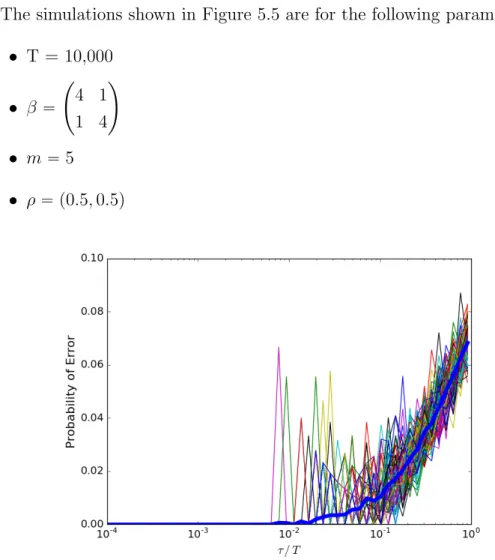
The simulations shown in Figure 5.5 are for the following parameters: • T = 10,000 • β “ ˜ 4 1 1 4 ¸ • m “5 • ρ“ p0.5,0.5q

Figure 5.5: Performance of message passing in recovering two equal-sized communities. The performance plot of 100 random graphs are shown, and the average performance is depicted by the bold blue curve.

From Figure 5.5, we observe that message passing successfully recovers all the first 100 vertex labels 98% of the time, and on average, makes an error on 5%.

(48)

CHAPTER 6 CONCLUSION

In this thesis, we have presented a study of community detection in preferen-tial attachment graphs. This study of a popular statistical problem on a new model proved to be an exciting area of research, as it provided a fertile ground for many new ideas, and also brought together interesting concepts from the SBM and the PA model. The random graph model was introduced, and some basic properties were examined. The degree-growth process, a novel viewpoint of tracking the time-evolution of the graph, was presented and a precise asymptotic characterization of the process was given. This analysis was then used to develop a hypothesis testing based algorithm for commu-nity recovery, for which an upper bound on the probability of error was given. The principles behind this algorithm were then extended to develop a mes-sage passing algorithm that runs on the graph to be clustered. The mesmes-sage passing algorithm was shown to have better performance for recovering a single planted community, and also gave a method to recover two equal-sized planted communities. These points were illustrated by simulations.

The thesis does not give a theoretical performance guarantee for the mes-sage passing algorithm. This remains an open question. The thesis also does not examine other algorithms for community detection, like SDP relaxations or spectral methods. We hope this shall be studied in the future. Finally, it is important to study when community recovery is and is not information-theoretically feasible.

(49)

REFERENCES

[1] S. Fortunato, “Community detection in graphs,” Physics Reports, vol. 486, no. 3-5, pp. 75–174, 2010.

[2] E. Abbe, “Community detection and stochastic block models: Recent developments,” arXiv preprint arXiv:1703.10146, 2017.

[3] “The graph of a social network,” https://griffsgraphs.wordpress.com/ 2012/07/02/a-facebook-network/, accessed: 2018-05-23.

[4] C. Moore, “The computer science and physics of community detec-tion: Landscapes, phase transitions, and hardness,” arXiv preprint arXiv:1702.00467, 2017.

[5] B. Hajek, Y. Wu, and J. Xu, “Achieving exact cluster recovery thresh-old via semidefinite programming,” IEEE Transactions on Information Theory, vol. 62, no. 5, pp. 2788–2797, 2016.

[6] E. Abbe, A. S. Bandeira, and G. Hall, “Exact recovery in the stochastic block model,” IEEE Transactions on Information Theory, vol. 62, no. 1, pp. 471–487, 2016.

[7] A.-L. Barab´asi and R. Albert, “Emergence of scaling in random net-works,” Science, vol. 286, no. 5439, pp. 509–512, 1999.

[8] B. Bollob´as, O. Riordan, J. Spencer, and G. Tusn´ady, “The degree se-quence of a scale-free random graph process,” Random Structures & Algorithms, vol. 18, no. 3, pp. 279–290, 2001.

[9] R. Van Der Hofstad, Random Graphs and Complex Networks. Cam-bridge University Press, 2016, vol. 1.

[10] J. Jordan, “Geometric preferential attachment in non-uniform metric spaces,”Electronic Journal of Probability, vol. 18, no. 8, pp. 1–15, 2013. [11] F. McSherry, “Spectral partitioning of random graphs,” in Foundations of Computer Science, 2001. Proceedings. 42nd IEEE Symposium on. IEEE, 2001, pp. 529–537.

(50)

[12] B. Hajek, Y. Wu, and J. Xu, “Recovering a hidden community beyond the spectral limit in Op|E|log˚_|_V_|q _time,” _{arXiv preprint}

arXiv:1510.02786, 2015.

[13] B. Hajek and S. Sankagiri, “Community recovery in a preferential at-tachment graph,” arXiv preprint arXiv:1801.06818, 2018.

[14] V. S. Borkar, Stochastic Approximation. Cambridge University Press, 2008.

[15] D. J. MacKay, Information Theory, Inference and Learning Algorithms. Cambridge University Press, 2003.

Community detection in preferential attachment graphs

ABSTRACT

ACKNOWLEDGMENTS

TABLE OF CONTENTS

CHAPTER 1

INTRODUCTION

1.1

Random graph models

1.1.1

Stochastic block model

1.1.2

Preferential attachment graphs

1.1.3

Preferential attachment graphs with planted

communities

1.2

Algorithms for community detection

1.2.1

Semi-definite programming

1.2.2

Spectral methods

1.2.3

Belief propagation

CHAPTER 2

THE RANDOM GRAPH MODEL

2.1

Model description

2.2

Half-edges and their convergence

2.3

The degree growth process

2.4

The

Z

-process

2.5

Asymptotic degree distribution

CHAPTER 3