Socioeconomic Institute
Sozialökonomisches Institut
Working Paper No. 1014
Why the Linear Utility Function is a Risky Choice in
Discrete-Choice Experiments
Michèle Sennhauser
Socioeconomic Institute
University of Zurich
Working Paper No. 1014
Why the Linear Utility Function is a Risky Choice in Discrete-Choice
Experiments
November 2010
Author's address:
Michèle Sennhauser
E.mail:[email protected]
Publisher
Sozialökonomisches
Institut
Bibliothek (Working Paper)
Rämistrasse 71
CH-8006 Zürich
Phone: +41-44-634 21 37
Fax: +41-44-634 49 82
URL: www.soi.uzh.ch
E-mail: [email protected]
Why the Linear Utility Function is a Risky Choice
in Discrete-Choice Experiments
Mich`
ele Sennhauser
∗November 22, 2010
Abstract
This article assesses how the form of the utility function in discrete-choice experiments (DCEs) affects estimates of willingness-to-pay (WTP). The utility function is usually assumed to be linear in its attributes. Non-linearities, in the guise of interactions and higher-order terms, are applied only rather ad hoc. This paper sheds some light on this issue by showing that the linear utility function can be a risky choice in DCEs. For this purpose, a DCE conducted in Switzerland to assess preferences for statutory social health insurance is estimated in two ways: first, using a linear utility function; and second, using a non-linear utility function specified according to model specification rules from the econometrics and statistics literature. The results show that not only does the non-linear function outperform the linear specification with regard to goodness-of-fit, but it also generates significantly different WTP. Hence, the functional form of the utility function may have significant impact on estimated WTP. In order to produce unbiased estimates of preferences and to make adequate decisions based on DCEs, the form of the utility function should become more prominent in future experiments.
Keywords: Discrete-Choice Experiment; Preference Measurement; Health Insurance; Model Specification
JEL classification codes: C52, C9, I11, I18
∗Department of Economics, University of Zurich, Hottingerstrasse 10, 8032 Zurich Switzerland.
1
Introduction
Discrete-choice experiments (DCEs) enjoy great popularity with the number of applied studies in-creasing steadily and penetrating every branch of the health-economic field (see Louviere and Lancsar (2009)). Methods of DCE are also improving. Improvements in designs, attribute choice, and ques-tionnaire methods have all recently emerged. For example, Green and Gerard (2009) were the first to implement cost-effectiveness of alternatives in the attributes. At the same time, more complex esti-mation procedures are being used. Whereas logit or probit estiesti-mations are most commonly applied, random coefficient models (also called mixed logits) are becoming more frequently used (Regier et al. (2009)).
One component of DCEs that remains unchanged during this process of improvement: the form of the utility function. Almost all studies refer to Louviere et al. (2000), who stated that a linear speci-fication in linear models typically accounts for 70 to 90 percent of explained variance. Consequently, most authors choose a main effects design and assume that all interactions are equal to zero (Amaya-Amaya et al. (2008), for an example, see Slothuus Skjoldborg and Gyrd-Hansen (2003)). Interactions are then implemented rather ad hoc, or in the guise of interactions with socioeconomic character-istics (see for example Gerard et al. (2008)). However, it can be argued that the utility function is unlikely to be linear because of diminishing marginal returns and gain-loss asymmetries (Hoyos (2010)). So far, there have only been small attempts in the DCE literature toward a non-linear specification. Ryan and Watson (2008) note that, at the design stage, the researcher should consider the form of the utility function, taking account of potential non-linearities. However, they then proceed only estimat-ing main effects, with interactions and higher-order terms assumed as negligible with the justification to be consistent with most DCE applications. Lancsar and Louviere (2006) outline difficulties with assuming linear utility functions. Because tests for dominance and lexicographic preferences rely on this assumption to hold, respondents previously labeled as ”irrational” may simply appear to be so due to the specification, but are in fact not. A number of studies go further by allowing for interactions. Linearity assumptions of particular attributes were tested using a Wald or a Likelihood-Ratio (LR) test (as for example Telser and Zweifel (2002)).
Among econometricians, there is an ongoing methodological debate about model specification, but so far there is no ”best” way of finding a correct model. As Kennedy (2003) notes, however, the debate has given birth to the general principle that economic theory should be the foundation of the model. Simultaneously, the data should help create a ”more informed” economic theory by using econometric misspecification tests. However, to the knowledge of the author, this way of specification has not been applied yet to DCEs.
This paper sheds some light on this issue by showing that the linear utility function can be a risky choice in DCEs. For this purpose, a DCE conducted by Becker (2006, Chapters 6-8) in Switzerland is re-examined. The experiment elicits willingness-to-pay (WTP) for debated options in Swiss manda-tory social health insurance. The DCE is evaluated in two ways. First, the utility function is assumed to be linear in the attributes; second, a non-linear utility function is used, employing econometric misspecification tests (as outlined by Hosmer and Lemeshow (2000)). The results are compared in terms of goodness-of-fit and estimated WTP. The findings suggest that not only the non-linear func-tion outperforms the linear specificafunc-tion with regard to goodness-of-fit, but also generates significantly different WTP. The results conclude that the form of the utility function may have significant impact on estimated WTP. In order to produce unbiased estimates of preferences, the specification of the utility function should be given more attention in future experiments.
The paper is organized as follows. Section 2 outlines the theoretical foundations of DCEs and model specification. Section 3 introduces the experiment and Chapter 4 presents the empirical results. Section 5 concludes.
2
Theoretical Foundations
2.1
Discrete-Choice Experiments
Based on random utility theory (see Luce (1959), Manski and Lerman (1977), McFadden (1974), McFadden (1981), and McFadden (2001)), DCEs are designed to investigate individuals’ preferences for (non-)marketed goods or goods that do not yet exist.
In a DCE, participants are repeatedly asked to choose between a fixed status quo and an alternative whose attributes take on different values each time. When choosing between alternatives, a rational individual will always select the alternative with the higher level of expected utility. Thus, neglecting the expectation operator for simplicity, the decision-making process functions as a comparison of utility values determined by
Uij ≡v(aj, pj, yi, si, εij), (1)
whereUij represents the indirect utility value attained by individualiin alternativej. It depends on
the vector of attributesaj, the pricepj, the individual’s incomeyi, and socioeconomic characteristics
denoted bysi. Finally,εij is an error term that varies over alternatives and individuals. Provided the
error term is additive, the individual will choose alternativekover alternativel if
u(ak, pk, yi, si) +εik≥u(al, pl, yi, si) +εil, (2)
where u(·) is the deterministic and εij the stochastic component of the utility function v(·). The
probability of choosing the alternativekoverl,Pik, is assumed to equal the probability of the difference
in equation (2) occuring. Solving for the difference in error terms, one obtains
Pik=P rob[εil−εik≤u(ak, pk, yi, si)−u(al, pl, yi, si)]. (3)
For any inference about the left-hand side of inequality (3), a probability law forω=(εil−εik) must
be assumed. Since the logistic distribution assumes independence of irrelevant alternatives (IIA), the normal distribution is used here, resulting in probit estimation. It is assumed that errors are correlated between the choices of a given respondent but not across respondents, calling for random effects specification. With the utility function linear in parameters (Louviere et al. (2000)), one has
∆Uik=β0+β1a1k+β2a2k+. . .+βLaLk+ωij, (4)
withωik=µi+νik. Here,a1k, ...,aLk are the L attributes of the alternative k in consideration .
Ac-cording to equation (3), only differences in utility matter. For this reason, fixed characteristics of
respondents drop out. Theβs are the parameters to be estimated. With a non-linear utility function,
interactions and higher-orders terms of the attributes are also in equation (4).
Based on Hanemann (1983), the marginal rate of substitution (MRS) between the two attributes
mandnis equal to the ratio of the derivatives of the indirect utility function with respect to the two
attributes. In the case of a linear utility function this is
M RS=∂v/∂am
∂v/∂an
= βm
βn
. (5)
Definingnas a financial attribute allows interpretation of the negative of the MRS as a marginal WTP
for attributem. With a non-linear utility function, the MRS is no longer constant and can only be
2.2
Specification of the Utility Function
As outlined in the introduction, economic theory should form the foundation of the utility function’s specification. Indeed, misspecification tests from the econometrics and statistics literature should help to create the model. Hosmer and Lemeshow (2000, Chapter 4) provide an overview of these methods and present a strategy for binary response models. In the following, their 5-step procedure is sum-marized with regard to DCEs. Steps 1, 2, and 5 concern the issue of choosing variables that belong in the utility function. If too many variables are included, the problem of over-fitting arises, typically characterized by unrealistically large estimates of coefficients and/or standard errors (see Harrell et al. (1996)). If an insufficient number of variables is included or variables that do not belong into the model are used, the generated predictions are also poor. Steps 3 and 4 concern the issue of choosing the attributes’ functional form.
Step 1: As a first step, Hosmer and Lemeshow (2000) propose a careful univariate analysis of each of the possible covariates for the model. In the case of DCEs, these are the attributes. Contingency tables, smoothed scatter plots, and LR tests are some of the instruments that can be used. After the researcher determines a general impression of the relations between the dependent variable (0 if the respondent decides in favor of the status quo, 1 if in favor of the alternative) and the independent variables (the attributes), a stepwise method may be applied to decide which attributes should be considered. It can either be a forward selection with a test of backward elimination or a backward elimination followed by a test for forward selection. According to Mickey and Greenland (1989), the significance level of entry into the model should not be equal to the traditional values (such as 0.05) because important variables could be excluded mistakenly. They recommend using a value between 0.15 and 0.25. However, most DCEs are designed and pretested in such a way that all attributes are important. Nevertheless, attributes can still find their way into the utility function despite insignifi-cance if they are important for answering the research questions.
Step 2: The second step is to verify all the attributes that survived the selection procedure of Step 1. This should first include a Wald statistic for each variable. Attributes that do not contribute to the model are then excluded and the new model is compared to the former using an LR test. Estimated coefficients should also be compared when excluding an attribute. If they change markedly in magni-tude, this indicates that the excluded variable was important for providing an adjustment of the effect of the attribute remaining in the model.
Step 3: Now that all attributes are verified, Hosmer and Lemeshow (2000) suggest exploring the scales of the continuous attributes. As a starting point, it is assumed that the utility function is linear in the covariates. There are different methods to ascertain this assumption, three of which follow. (1) A univariate smoothed scatter plot (Cleveland (1979) and Cleveland and Devlin (1988)) shows potential non-linearities in the data and can easily be performed using statistical packages. (2) Four dummy variables (”design variables”) are generated for the quartiles of the attribute. These are re-gressed together with the other attributes (but without the attribute in consideration and the first quartile’s dummy) on the dependent variable. The quartiles’ means are plotted against the estimated coefficients of the dummies. For the first quartile, the coefficient is set to zero. The shape of this curve shows whether the linear specification might be appropriate. (3) The modified Hosmer-Lemeshow test (see Section 2.3 below), which can be applied for each variable separately. If this test fails, the linear specification is probably incorrect.
Step 4: In principle, the utility function needs to be as rich as the data requires, including the possibilities of interactions of higher order. However, all possible interactions should not be done in a model with many attributes, because this implies a very high-order regression. Consequently, the fourth step is to assess the need to include interaction terms. All possible interactions are tested using LR tests. To verify the results of Step 3, the terms in squares and other higher orders that resulted from Step 3 are tested as well.
Step 5: As a last step, in addition to assessing goodness-of-fit of the specified utility function, Hosmer and Lemeshow (2000) propose to backwardly select for more parsimony. However, the final
backward selection has to carefully consider the fit of the model. If too many interactions and higher-order terms are dismissed, the utility function may no longer pass the goodness-of-fit tests.
2.3
Assessing Goodness-of-Fit
To decide which utility function is ”better”, linear or non-linear, a variety of goodness-of-fit measures are available. These include the LR test, the Akaike Information Criterion (AIC), the Bayesian Infor-mation Criterion (BIC), and the log-likelihood. However, the following tests for misspecification can also be used, as proposed by Basu et al. (2004) and Basu et al. (2006).
• Pregibon’s Link test (see Pregibon (1980) and Pregibon (1981)): This is a parsimonious test
for non-linearity. Based on the initial estimate of the regression coefficients, a prediction of the dependent variable is generated. The prediction and the prediction squared are included as the only covariates in a second version of the model. If the specification is truly linear, then the coefficient of the squared term should not be significantly different from zero.
• Ramsey’s Reset test (see Ramsey (1969)): The Reset test allows for a richer form of model failure
than the Link test. By including not only the prediction and the prediction squared but also the cube and prediction to the power of four, it allows for an s-shaped misfit compared to only a quadratic misfit with the Link test.
• Copas test (see Copas (1983)): This is a split-sample, cross-validation test for over-fitting the
data. The sample is randomly divided into estimation data and test data. From a regression using the first sample, the predicted values are saved. These are used as the only covariate in a regression with the test data set. If the coefficient of the predictions is significantly different from one, over-fitting is a problem.
• Modified Hosmer-Lemeshow test (see Hosmer and Lemeshow (2000)): By observing the pattern
in the residuals of the estimation as a function of the predicted values, this test determines whether there is a systematic bias. The modified Hosmer-Lemeshow test regresses the residuals
on dummies for the deciles1 of the predicted values. An F-test shows if the dummies have a
significant influence on the residuals. If so, there is a non-linearity in the underlying data that is not represented in the model. The pattern of the regression coefficients and their standard errors allow a conclusion about the appropriate non-linear specification.
• Regular Hosmer-Lemeshow test (see Hosmer and Lemeshow (1980)): As with the modified version
the predicted values are grouped into ten equal sized groups. A Pearson-χ2-statistic compares
the observed and estimated expected frequencies and points out possible lacks of fit.
• Pearson correlation: A Pearson correlation significantly different from zero between the residuals
and the predicted values indicates that the model’s predictions are biased.
3
The Experiment
3.1
Background: Swiss Statutory Social Health Insurance
The DCE assesses preferences for Swiss statutory health insurance and WTP for proposed reforms.
It was conducted by Becker (2006, Chapters 6-8) in 2003.2 Switzerland is a country of interest
be-cause its health insurance combines mandatory and choice elements in a way similar to the US and the Netherlands (OECD (2004)). The Health Insurance Law (KVG), effective since 1996, obliges all permanent residents of Switzerland to purchase health insurance policies for basic coverage. The law defines a uniform basic package of health care benefits that has become more comprehensive over the years, mostly driven by technological progress and new treatment methods. For a new therapy or pharmaceutical product to be included in the benefit package, its effectiveness, efficacy, and economic efficiency have to be proven (Article 32 Health Insurance Law KVG). Premiums are community-rated 1 Depending on the size of the data set, the test can be performed with more than ten groups.
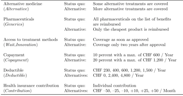
Table 1: DCE attributes, labels and levels
Alternative medicine Status quo: Some alternative treatments are covered
(Alternative) Alternative: More alternative treatments are covered
Pharmaceuticals Status quo: All pharmaceuticals on the list of benefits
(Generics) are reimbursed
Alternative: Only the cheapest product is reimbursed
Access to treatment methods Status quo: Coverage as soon as approved
(Wait Innovation) Alternative: Coverage only two years after approval
Copayment Status quo: 10 percent with a max. of CHF 600 / Year
(Copayment) Alternative: 20 percent with a max. of CHF 1,200 / Year
Deductible Status quo: CHF 230, 400, 600, 1,200, 1,500 / Year
(Deductible) Alternatives: CHF 0, 2,400, 4,800 / Year
Health insurance contribution Status quo: Individual contribution
(Contribution) Alternatives: CHF –50, –25, –10, +10, +25, +50 / Month Note: 1 CHF≈0.82 US$ at 2005 exchange rates
and not tax-financed, i.e. all insureds pay approximately the same independent of age and morbidity. In addition, there is a fixed rate of copayment, amounting to 10 percent of health care expenditures
with a maximum of CHF 600 per year (1 CHF≈0.82 US$ at 2005 exchange rates).3 Complementing
these mandatory elements, there are elements of choice. There is free choice of health insurer. Con-trary to the US, employers are not involved in this decision. Insurers are obliged by law to accept any applicant (for mandatory insurance, but not for supplementary health insurance). When it comes to choice of contract, there are two main elements. The first choice is the level of annual deductible.
It ranges from a minimum of CHF 300 to a maximum of CHF 1,500.4 The second involves choosing
between the conventional and Managed Care (MC) options. In the standard case, the choice of the provider is not restricted. In the MC settings, alternatives are offered. These include physician net-works (similar to Independent Provider Associations in the US), restricted lists of physicians (Preferred Provider Organizations) and Health Maintenance Organizations (HMOs). For MC options, insurers are allowed to give reductions in premiums up to a certain percentage. However, the basic package of benefits remains the same, independent of the deductible and model chosen.
3.2
Attributes
The DCE’s attributes represent different aspects of health insurance contracts within the context of Swiss health insurance (see Table 1). The importance of the attributes was secured by discussions with various experts from the Swiss health care system. Further data comes from a survey conducted by the Swiss Society of Applied Social Research (GFS (2001)). The first attribute of interest is reimbursement
of alternative medicine (Alternative). In the status quo insurance contract, acupuncture, traditional
Chinese medicine, anthroposophic medicine, homeopathy, neural therapy, and phytotherapy are part of the benefit package. The alternative suggests more treatments be reimbursed, such as treatments of alternative practitioners and naturopathy. The second attribute is reimbursement of pharmaceuticals (Generics). Whereas in the status quo insurance contract, where all pharmaceuticals on the list of benefits are reimbursed, the alternative offers only the cheapest product (the generics) to be paid by
the health insurer. Another constraint is access to treatment methods (Wait Innovation). While in
the status quo contract, access is guaranteed to all insureds immediately after approval, the alterna-tive allows coverage only after 2 years. Two issues of great interest in the ongoing reform debate are 3 The maximum was increased to CHF 700 per year in 2004.
consumers’ willingness-to-accept copayment (Copayment) and deductibles (Deductible). With a co-payment rate of 10 percent and a maximum co-payment of CHF 600 per year, the status quo’s coco-payment rate is lower than the alternative’s, which offers a 20 percent rate and a maximum of CHF 1,200 per year. For the deductible, there are five options, ranging from CHF 230 up to CHF 1,500 per year. The alternatives offer a wider range, starting from no deductible at all to CHF 4,800 per year. The
sixth attribute is health insurance contributions (Contribution). The amount of contribution varies
by increases and decreases of up to CHF 50 per month in the alternatives.
3.3
Pretest and Design
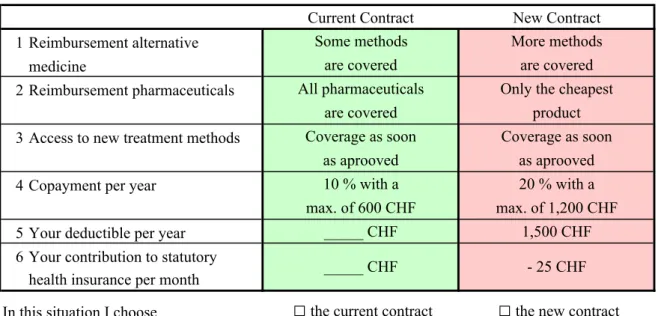
These and other attributes were checked for relevance in a pretest conducted with 20 individuals. The respondents understood the survey well and did not find the DCE section difficult. However, an ad-justment had to be made with the deductible. While the levels for the alternative were CHF 3,000 and CHF 6,000 in the pretest, these were lowered to CHF 2,400 and CHF 4,800 to avoid protest response for lack of realism. For the main survey, the number of possible scenarios was reduced from a full factorial design to a fractional factorial D-optimal design (see Atkinson and Donev (1992), Street et al. (2001), Burgess and Street (2003), and Carlsson and Martinsson (2003)) of 27 choice sets using the program GOSSET (see Kuhfeld et al. (1994) and Sloane and Hardin (2007)). Because the intention was to assess interactions and higher-order terms, all possible interactions and higher-order terms up to the power of five were implemented in the design. The 27 choice sets were split randomly into three groups of nine choices each. One choice was included twice in each choice set for consistency checking (Ryan and Bate (2001)), resulting in ten choices per person. In each choice set, the respondents are presented with their (constant) individual status quo and one alternative. Figure 1 shows an example. To avoid learning or fatigue effects, the order of the choice alternatives was randomly changed (Kjær et al. (2006)). Some 60 percent of respondents deviated from their status quo at least once. This means that around 40 percent of respondents never chose the alternative insurance contract. In total, 18 percent of the decisions were made in favor of the alternative. As for the consistency test, the choice included twice was ”incorrectly” chosen by only 13 of 1,000 respondents. Overall, the observed choices are plausible. Respondents tend to opt for the objectively ”good” alternatives and to reject the ”bad” alternatives among the ten choices given.
Choice Question: Which insurance contract do you prefer?
Current Contract New Contract 1 Reimbursement alternative Some methods More methods
medicine are covered are covered
2 Reimbursement pharmaceuticals All pharmaceuticals Only the cheapest
are covered product
3 Access to new treatment methods Coverage as soon Coverage as soon as aprooved as aprooved
4 Copayment per year 10 % with a 20 % with a
max. of 600 CHF max. of 1,200 CHF
5 Your deductible per year _____ CHF 1,500 CHF
6 Your contribution to statutory health insurance per month
In this situation I choose
□
the current contract□
the new contract_____ CHF - 25 CHF
3.4
Sample and Interview Strategy
The survey was conducted in Summer 2003 and consisted of 1,000 telephone interviews. Participants were chosen as representative with respect to age, gender, language (the German and the French speaking parts of Switzerland), education, professional status, and rural or urban residence. The sur-vey contained two steps. After individuals agreed to participate, they were asked to look up their personal monthly contributions and their annual deductible to their insurance plan. This guarantees the respondents’ knowledge of the status quo, which is essential for making an informed choice be-tween the current contract and a proposed alternative. The participants were also sent an information package, containing descriptions of the attributes. The second step was the DCE itself. Participants were asked to compare the fixed status quo against a hypothetical alternative defined by the attributes mentioned above. The procedure was replicated ten times. Other questions concerned utilization of health care services, preferences for new elements in the insurance package, and socioeconomic char-acteristics such as age, gender, household income, and education.
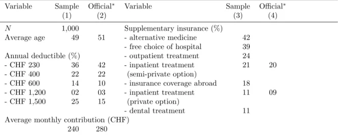
Table 2 shows selected descriptive statistics. Individuals with a low deductible are somewhat un-derrepresented and individuals with a high deductible are overrepresented. On the whole, however, the distribution of the annual deductible is representative when compared with official data (columns (2) and (4)). Since one attribute of interest is coverage of alternative treatment methods, supplemen-tary health insurance is presented as well. 42 percent of the interviewed individuals buy insurance for alternative medicine treatments, making this the most popular supplementary health insurance. Another important dimension is additional coverage of inpatient treatment. 21 percent of individuals have semi-private and 11 percent private accommodation covered by hospital supplementary insur-ance. In statutory health insurance, basic inpatient services are covered only in hospitals located in the canton of residence. 39 percent of those interviewed buy insurance for free choice of hospitals in all Swiss cantons. The average monthly contributions are CHF 240 in the sample and CHF 280 in official statistics. The discrepancies are explained by three reasons. First, the official statistics include only the (expensive) contracts with the lowest deductible, whereas the sample also includes (less expensive) contracts with higher deductibles and MC alternatives. Second, the canton Ticino, which has tradi-tionally high health care expenditures and also high premiums, is not included in this sample. Third, the official figure includes contributions to accident insurance, which were excluded here.
Table 2: Selected descriptive statistics
Variable Sample Official∗ Variable Sample Official∗
(1) (2) (3) (4)
N 1,000 Supplementary insurance (%)
Average age 49 51 - alternative medicine 42
- free choice of hospital 39
Annual deductible (%) - outpatient treatment 24
- CHF 230 36 42 - inpatient treatment 21 20
- CHF 400 22 22 (semi-private option)
- CHF 600 14 10 - insurance coverage abroad 18
- CHF 1,200 02 03 - inpatient treatment 11 09
- CHF 1,500 25 15 (private option)
- dental treatment 11
Average monthly contribution (CHF)
240 280
Note: ∗ Swiss Population 2003. Source: Federal Office of Public Health (2005); 1 CHF ≈ 0.82 US$ at 2005 exchange rates
4
Empirical Results
4.1
Specification of the Utility Function
To compare the linear with a non-linear utility function, the non-linearities have to be specified first. Using the data from the DCE presented above, the procedure by Hosmer and Lemeshow (2000) is performed step-by-step as outlined in Section 2.2. The results can be summarized as follows.
Step 1: After a univariate analysis of each attribute (not shown here), a forward selection probit estimation with a test of backward elimination is performed. The significance level of entry is set at 0.25 and the level to remove at 0.2. All attributes are approved to belong in the utility function.
Step 2: The multivariate model is estimated and each attribute is then tested according to Step 2 in Section 2.2. All attributes prove significance.
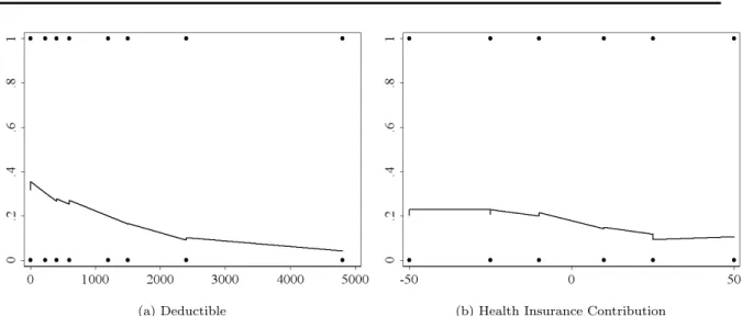
Step 3: Method (1): For the continuous variablesDeductible andContribution, a smoothed
uni-variate scatter plot is estimated (see Figure 2). Smoothing is performed with the locally weighted regression command ”lowess” in Stata 10.1. Neither attribute bears a linear relation with the
depen-dent variable. The plot forDeductiblesuggests adding a quadratic term. The plot forContributionis
non-linear, too. This may call for a cubic term. However, as the result is not conclusive, comparison with results of further steps is required.
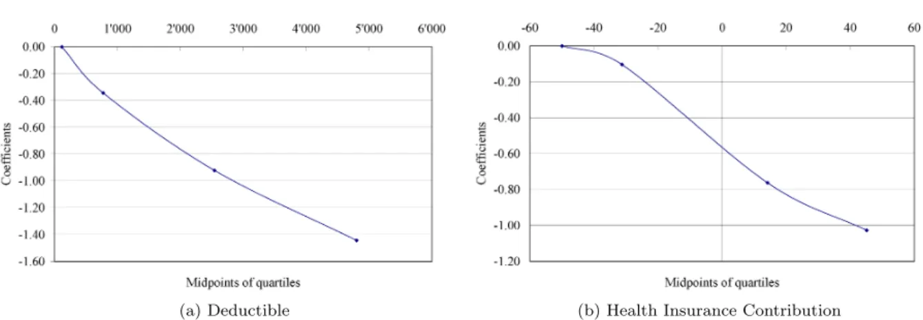
Method (2): Figure 3 shows the results of the second method to explore the scale of continuous
variables by ”design variables” (see Step 3 in Section 2.2). The quartiles’ midpoints of Deductible
andContribution, respectively, are plotted against the estimated probit regression coefficients of the dependent variable (0 if the respondent opted for the status quo, 1 otherwise) on all attributes, with
DeductibleandContributionsubstituted by dummy variables for the quartiles. The plot forDeductible
shows a linear function with only a slight curvature (see Figure 3a). This may indicate a non-linear
specification or just a deviation with non-significant implications. The plot forContribution suggests
a non-linear, s-shaped relationship (see Figure 3b).
Method (3): The third method is the modified Hosmer-Lemeshow test (see Section 2.3). For
Deductible, the test is performed with dummies for 1/8 of the predicted values, and forContribution
with dummies for 1/6 of the predicted values. Both F-statistics show that there is a systematic pat-tern between the residuals and the particular attribute (both p-values of the F-statistics are 0.00).
According to these results,DeductibleandContribution should not be specified as linear.
(a) Deductible (b) Health Insurance Contribution
(a) Deductible (b) Health Insurance Contribution Figure 3: Plot of estimated probit regression coefficients versus approximate quartile midpoints of
DeductibleandContribution
Note: Coefficients are from a regression of the dependent variable (0 if the respondent opted for the status quo, 1 if he or she opted for the alternative) on three dummies for the second, third, and fourth quartiles ofDeductible and Contribution, respectively, and the remaining attributes. In the plot the coefficient of the first quartile’s dummy is set to zero.
Step 4: To test for interactions, the LR test is used. Every possible interaction between the at-tributes is tested. For evidence about the functional form of the atat-tributes, the LR test is also performed for terms of second and higher orders. The interactions proven to be significant are presented in Table 3.
Summarizing the findings from Steps 3 and 4, the Deductible smoothed scatter plot suggests a
squared specification (see Figure 2a). Figure 3a favors a linear or quadratic form. Whereas these methods do not draw a final conclusion (the deviations could be non-significant implications for the specification), the modified Hosmer-Lemeshow test clearly favors a non-linear utility function. The LR tests in Step 4 support this finding. According to the LR test, both a squared and a cubic term significantly contribute to an improvement of fit. Backward selection procedures and goodness-of-fit tests are required to decide the final specification.
The smoothed scatter plot forContribution(see Figure 2b) and the ”design variables” (see Figure
3b) suggest a non-linear specification. The Hosmer-Lemeshow test confirms this result. However, it is unclear how many higher-order terms should be included. The LR tests suggest going to the fourth power. Backward selection and goodness-of-fit tests are also required for the final specification of this attribute.
Step 5: A backward selection procedure is performed and the results are assessed in view of goodness-of-fit. The most parsimonious utility function that still passes all specification tests is the
following: Besides all main effects, interactions are Alternative × Copayment, Wait Innovation ×
Generics,Copayment×Generics,Wait Innovation×Contribution, andCopayment×Contribution
Table 3: Interactions and terms of second and higher order resulting from Step 4
Copayment×Alternative Wait Innovation ×Generics Copayment×Generics Wait Innovation ×Contribution Copayment×Contribution Alternative×Contribution Contribution2 Deductible2
Contribution3 Deductible3
Contribution4
(note thatAlternative×Contributionis dropped compared to Table 3). Deductiblehas to be included
in squares andContribution to the power of four. This will later be referred to as the ”non-linear”
utility function, as opposed to the ”linear” utility function containing the main effects only.
4.2
Comparison of Goodness-of-Fit
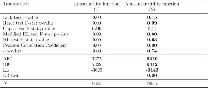
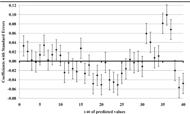
In this section, the utility functions are compared with regard to goodness-of-fit. The results of the tests presented in Section 2.3 are shown in Table 4. The linear specification fails in all but one test (see column (1)). Neither the Link, the Reset, nor one of the Hosmer-Lemeshow tests support the linear utility function. This specification only passes the Copas test. However, this was expected, since Copas is a test for over-fitting the data and the model is very parsimonious, containing only the main effects. The non-linear utility function passes all the tests presented. Only the Reset test might attract attention, with a p-value of 0.09. Strict adherence to a 10 percent level of statistical signif-icance would point out a possible s-shaped misfit. However, considering the richness of the data set (1,000 respondents with ten decisions each, resulting in 10,000 observations), it is important not to rely too strictly on test statistics. The p-value most likely does not point out a significant misfit in this case. Performing the modified Hosmer-Lemeshow test, the size of the data set allows the building of 40 groups, each comprising 2.5 percent of the predicted values. Figure 4 presents the coefficients from regressing the residuals (from a regression of the dependent variable on the attributes’ main effects (Figure 4) or the main effects and the additional variables for non-linearity (Figure 5), respectively) on dummies for the 40 groups. If there was no misspecification, the coefficients would be distributed ran-domly among the zero-line. However, Figure 4 shows a systematic u-shaped pattern. Consequently, the linear specification fails the test of no misfit. The pattern for the non-linear utility function (see Figure 5) passes the test with a p-value of 0.80 when testing the residuals to be zero jointly. From Figure 5, the coefficients are seen to be distributed close to randomly among the zero-line. Both the Akaike and Bayesian information criteria prefer the non-linear utility function, as well as the log-likelihood. An LR test shows that the added variables significantly contribute to a better fit of the utility function.
Table 4: Comparison of goodness-of-fit results linear and non-linear utility function
Test statistic Linear utility function Non-linear utility function
(1) (2)
Link test p-value 0.00 0.15
Reset test F-stat p-value 0.00 0.09
Copas test F-stat p-value 0.90 0.71
Modified HL test F-stat p-value 0.00 0.80
HL test F-stat p-value 0.00 0.63
Pearson Correlation Coefficient 0.03 0.00
- p-value 0.00 0.74 AIC 7272 6320 BIC 7322 6442 LL -3629 -3143 LR test 0.00 N 9655 9655
Note: AIC is the Akaike Information Criterion and BIC is the Bayesian Information Criterion. LL is the log likelihood, evaluated at the maximum likelihood estimator. Boldface entries indicate the better specification for the particular criterion.
Figure 4: Regression result modified Hosmer-Lemeshow test linear utility function
Figure 5: Regression result modified Hosmer-Lemeshow test non-linear utility function Note: Coefficients are from a regression of the residuals on dummy variables for 1/40 of the predicted values.
T able 5: Marginal WTP with linear an d non-linear sp ecification of the utilit y function, (CHF p er mon th) Linear Sp ecification Non-lin e ar Sp ecification Difference t-statistic † Standard Errors Standard Errors A ttribute WTP l Delta Metho d Bo otstrap W T Pn Delta Metho d Bo otstrap (1) (2) (3) (4) (5) (6) (7) (8) Constan t -31.87 ∗∗∗ 4.55 4.92 -30.52 ∗∗∗ 11.71 13.94 -1.35 0.13 Alternativ e 1 23.89 ∗∗∗ 3.09 3.46 11.70 ∗∗∗ 5.28 5.58 12.19 2.52 Generics 2 -12.47 ∗∗∗ 3.03 3.26 -29.03 ∗∗∗ 7.28 7.35 16.56 2.69 W ait Inno v ation 3 -39.40 ∗∗∗ 3.34 3.79 -38.11 ∗∗∗ 5.89 6.25 -1.29 0.15 Copa ymen t 4 -19.08 ∗∗∗ 3.00 3.38 -31.71 ∗∗∗ 4.49 4.43 12.63 3.02 Deductible 5 -00.03 ∗∗∗ 0.00 0.00 -00.04 ∗∗∗ 0.01 0.01 0.01 1.51 1 Reim bursemen t of more alterna ti v e treatmen t metho ds (a lterna ti v e practitioner and naturopath y) 2 Reim bursemen t of only the cheap est pharmaceutical 3 Co v erage only tw o y ears after appro v al 4 20 p ercen t with a max. of CHF 1,200 / Y ear 5 Choice b et w een CHF 0, 2,400, and 4,800 / Y ear Note: *** indicates significance at the 1 p ercen t lev el; †: t-test statisti cs from one b o otstrap with b oth mo dels e stimated sim ultaneously , nr. of iterations = 1,000, no bias correction required (see Ef ron and Tibshirani (1993)), no acceleration; 1 CHF ≈ 0.82 US$ at 2005 exc hange rates
4.3
Comparison of Willingness-to-Pay
In this section, the utility functions are compared with regard to estimated WTP. If there is no signif-icant difference, the linear utility function can be seen as a good approximation. If the results differ significantly, it emphasizes the necessity to apply statistical specification rules in DCE analysis.
Table 5 shows the estimated WTP values for the linear utility function (WTPl, column (1)) and the
non-linear utility function (WTPn, column (4)).5 All WTP are calculated in terms of health insurance
contributions, i.e. βn in equation (5) is the coefficient of the attributeContribution. Because WTP is
not constant with the non-linear utility function, the estimated values are stated subject to the other attributes being equal to the status-quo level. Columns (2) and (5) of Table 5 show standard errors ac-cording to the delta method. As Mullahy and Manning (1996) note in the context of cost-effectiveness analysis, the delta method does not work well in the case of ratios. They present two safe strategies for calculating confidence intervals of ratios, one of which is bootstrapping. For this purpose, both utility functions have been bootstrapped simultaneously with 1,000 iterations (see columns (3) and (6) for the standard errors). This approach allows comparison of the estimates directly, t-testing the bootstrapped differences in WTP. This result is shown in column (8) of Table 5.
With both utility functions, the estimated WTP values are significantly different from zero.
How-ever, the difference between WTPland WTPn is of considerable magnitude and is statistically
signifi-cant in three out of five attributes. (1) The linear approach suggests that the respondents are willing to
pay CHF 24 per month for the coverage of more alternative treatment methods (Alternative). With
the non-linear specification, this value decreases to CHF 12 per month. (2) For a more restrictive
reimbursement of pharmaceuticals (Generics), respondents have to be compensated with a reduction
in health insurance contributions of CHF 13 per month when estimating the linear specification. This willingness-to-accept more than doubles to CHF 29 when using the non-linear function. (3) Concerning
financing, respondents ask for a reduction of CHF 19 in health insurance contributions (WTPl) with
an increase in the copayment rate (Copayment) from 10 to 20 percent. With the non-linear
specifica-tion, respondents ask for a reduction of CHF 32 per month. However, the differences in compensation
for delayed coverage of treatment methods (Wait Innovation), a marginal increase in the deductible
(Deductible), and the difference in the status-quo bias (Constant) are small and non-significant. The specification of the utility function has considerable effect on estimated WTP. The conse-quences of using the linear specification as a simplification can be striking. In the case of the presented DCE, these might include the following. (1) A health insurer might launch an alternative contract reimbursing more alternative treatment methods for an increase in premiums of CHF 24 per month (assuming this amount covers costs). The number of people actually buying the contract will be much lower than expected, because enrollees are willing to pay, on average, an increase of only CHF 12 per month for the additional benefits. (2) The regulator may propose to reimburse only the cheapest pharmaceutical product on the list of benefits and to decrease health insurance premiums by CHF 13 per month. However, the decrease in contributions is lower than the amount people ask for cuts in benefits. Inefficiencies result. (3) One may propose to decrease health insurance contributions by CHF 19 per month in exchange for an increase in the copayment rate from 10 to 20 percent and a maximum of CHF 1,200 instead of CHF 600 per year, with the advantage of mitigating moral hazard. However, the results show that respondents ask for higher compensation (CHF 32 per month) to accept this increase. This proposition might thus cause inefficiencies.
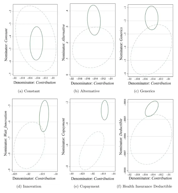
Simultaneously bootstrapping the linear and non-linear utility functions allows the comparison of
the two sets of WTP values. Figure 6 shows 95-percent confidence ellipses,6 where the solid line
corresponds to the linear function and the dashed line to the non-linear utility function. The x-axes 5 For the estimated coefficients see Table 6 in the Appendix. The coefficients of the higher-order terms are rather small, but nevertheless significantly different from zero. A specification neglecting these terms was tested for the sake of parsimony. However, in this case the Reset test signals a clear misfit, as does the (modified) Hosmer-Lemeshow test.
6 The estimated coefficients are normally distributed by assumption. Linear combinations of normal random variables are normally distributed as well, and so Figure 6 shows bivariate normal distributions. These belong to the elliptical family (McNiel et al. (2005)). This makes the confidence curves ellipses.
(a) Constant (b) Alternative (c) Generics
(d) Innovation (e) Copayment (f) Health Insurance Deductible
Figure 6: 95 percent confidence ellipses for marginal WTP
Note: Solid line = linear utility function, (de)nominator is equal to estimated coefficient of equation 4; dashed line = non-linear utility function, (de)nominator is equal to estimated coefficient (nominator: Constant,Alternative,Generics) or linear combination of coefficients (nominator:Wait Innovation,Copayment,Deductible; denominator:Contributions).
are the denominators of the marginal WTP (where the marginal WTP is equal to the marginal rate of substitution, see equation (5)). The y-axes are the numerators. In the case of the linear utility
function, the axes equal the single estimated coefficients (the x-axis is always equal to Contribution,
the y-axes vary). In the case of the non-linear utility function, the x-axes are single coefficients (for
Constant, Alternative, Generics) or combinations of coefficients (for Wait Innovation, Copayment, andDeductible). The y-axes are combinations of coefficients for all attributes in this case.
From Table 5, it can be seen that the standard errors become larger with the non-linearities. This increase is visible in Figure 6 as well, where the ellipses become larger. The positions of the pairwise ellipses provide information about the origin of differences in WTP estimates. For example, in the plot for the coverage of alternative treatment methods (Figure 6b), the origins of the two ellipses have almost the same x-coordinate, but different y-coordinates. The decrease in WTP from CHF 24
Hence, respondents value a marginal increase inContribution almost the same. However, coverage of additional treatment methods is valued less with the non-linear specification than with the linear. The
same holds forGenerics(Figure 6c), where the increase in willingness-to-accept from CHF 13 to CHF
29 per month results mostly fromGenerics. In the case of Copayment(Figure 6e), the valuation of
both attributes changes with the specification. The x- and the y-coordinates are shifted. This is due
to the interaction termCopayment×Contributions.7
5
Conclusions
When estimating willingness-to-pay (WTP) using discrete-choice experiments (DCEs), the utility func-tion is most commonly assumed to be linear in the attributes. Interacfunc-tions and higher-order terms are set to zero with reference to Louviere et al. (2000). Non-linearities are only implemented if they are of special interest or in the guise of interactions with socioeconomic characteristics to investigate heterogeneity in preferences. This paper addresses the issue of the utility function’s form by showing that the linear approximation can be a risky choice in DCEs. For this purpose, an experiment con-ducted by Becker (2006, Chapters 6-8) in Switzerland is re-examined. The DCE assesses preferences for Swiss statutory health insurance and WTP for proposed reforms. The attributes describe changes in the list of benefits (inclusion of additional alternative treatment methods, reimbursement of only the cheapest pharmaceuticals (generics), delayed access to new treatment methods and changes in financing (increased copayment rate, change in deductible and health insurance contributions).
The DCE is estimated in two ways, first using a linear utility function, including the main effects only, and second using a non-linear utility function, allowing for interactions and terms of higher-order. The procedure of Hosmer and Lemeshow (2000) is used for the specification of non-linearities, following the statistical model-specification literature. In a first step, the utility functions are tested for misfits, using a variety of goodness-of-fit measures as proposed by Basu et al. (2004) and Basu et al. (2006). The linear utility function is found to perform better with regard to over-fitting, but to have serious misfit problems. However, the non-linear utility function is found to present the data well. In a second step, the utility functions are compared with regard to estimated WTP, stated in terms of health insurance contributions. The results are found to significantly differ in terms of statistical significance and in magnitude for three out of five attributes. (1) With the linear utility function, respondents are willing to pay CHF 24 per month for the reimbursement of additional alternative
treatment methods. With the non-linear specification, estimated WTP decreases to CHF 12 per
month. (2) The linear specification proposes that respondents must be compensated with a decrease in contributions of CHF 12 per month in order to accept the reimbursement of only the cheapest pharmaceuticals (generics). However, this willingness-to-accept more than doubles with the non-linear utility function at CHF 29 per month. (3) An increase in the copayment rate from 10 to 20 percent with a simultaneous increase in the maximum copayment from CHF 600 to CHF 1,200 per year must be compensated with a decrease in contributions of CHF 20 per month with the linear specification, but rises to CHF 32 per month with the non-linear specification.
These findings suggest that the form of the utility function can have significant impact on estimated WTP. Using the linear specification as an approximation may lead to seriously biased estimates. Since DCEs are playing an increasingly significant role in health care decision making, the assumption of a linear utility function may lead to inefficient use of health care resources.
7 The ellipses can also be interpreted as visual indicators of correlation (SAS Institute Corp. (1999)). An ellipse collapses diagonally as the attributes become perfectly positively or negatively correlated. In case of uncorrelated attributes, the ellipse is circular or the orientation is aligned with a coordinate axis. If the ellipse’s orientation is to the northeast or the southwest quadrant, the attributes are positively correlated. If it is towards the northwest or the southeast quadrant, there is negative correlation. Further, from the orientation of the ellipses, it can be seen whether the 95-percent confidence regions are likely to include the origin or not. If this were the case, then the delta method approximation would fail (see Gleser and Hwang (1987)). The Fieller method would provide the appropriate alternative (see Fieller (1954), and for applications e.g. Willen and O’Brien (1996) or Heitjan (2000)).
However, this research is subject to several limitations. It can be argued that the linear functional form is a poor approximation in this setting, but might sufficiently serve in others. Also, there is no ”best” way of finding an appropriate model specification. The methodological debate is still ongoing, and will certainly continue into the future. A disadvantage of the procedure presented here is that finding the non-linearities is very time-consuming. The limiting factor is not computer power but rather creativity in finding a model that passes all specification tests simultaneously. Finally, the form of the utility function is one among many aspects of DCEs that need further consideration. Issues range from questionnaire development and choosing experimental designs to applications of new econometric methods (for a summary see Louviere and Lancsar (2009) or Hoyos (2010)). However, given the significant differences in estimated WTP, the form of the utility function is an important issue in DCE analysis which should be taken into account for future DCEs.
Appendix
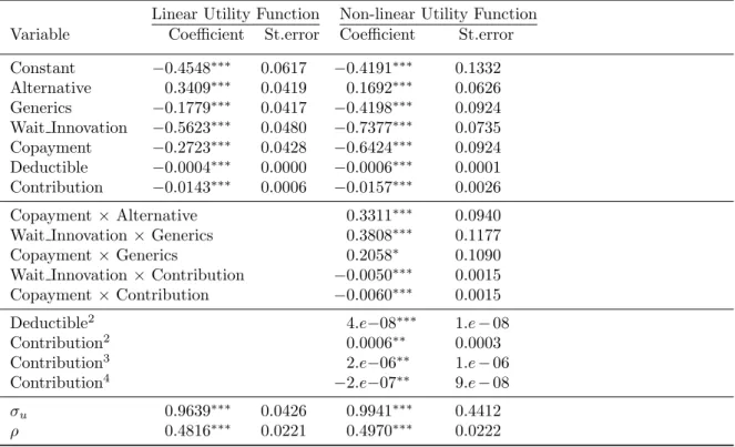
Table 6: Coefficients with standard errors, linear and non-linear utility function
Linear Utility Function Non-linear Utility Function
Variable Coefficient St.error Coefficient St.error
Constant −0.4548∗∗∗ 0.0617 −0.4191∗∗∗ 0.1332 Alternative 0.3409∗∗∗ 0.0419 0.1692∗∗∗ 0.0626 Generics −0.1779∗∗∗ 0.0417 −0.4198∗∗∗ 0.0924 Wait Innovation −0.5623∗∗∗ 0.0480 −0.7377∗∗∗ 0.0735 Copayment −0.2723∗∗∗ 0.0428 −0.6424∗∗∗ 0.0924 Deductible −0.0004∗∗∗ 0.0000 −0.0006∗∗∗ 0.0001 Contribution −0.0143∗∗∗ 0.0006 −0.0157∗∗∗ 0.0026 Copayment×Alternative 0.3311∗∗∗ 0.0940
Wait Innovation×Generics 0.3808∗∗∗ 0.1177
Copayment×Generics 0.2058∗ 0.1090
Wait Innovation×Contribution −0.0050∗∗∗ 0.0015
Copayment×Contribution −0.0060∗∗∗ 0.0015 Deductible2 4.e−08∗∗∗ 1.e−08 Contribution2 0.0006∗∗ 0.0003 Contribution3 2.e−06∗∗ 1.e−06 Contribution4 −2.e−07∗∗ 9.e−08 σu 0.9639∗∗∗ 0.0426 0.9941∗∗∗ 0.4412 ρ 0.4816∗∗∗ 0.0221 0.4970∗∗∗ 0.0222 Note: *** indicates significance at the 1, ** at the 5, and * at the 10 percent level
Acknowledgment
The author gratefully acknowledges econometric advice by Willard G. Manning (University of Chicago, USA) and helpful suggestions by Peter Zweifel (University of Zurich, Switzerland).
References
Amaya-Amaya, M., Gerard, K., Ryan, M., 2008. Discrete choice experiments in a nutshell. In: Ryan, M., Gerard, K., Amaya-Amaya, M. (Eds.), Using Discrete Choice Experiments to Value Health and Health Care. Springer, Dordrecht, Ch. 1, pp. 13–46.
Atkinson, A., Donev, A., 1992. Optimum Experimental Designs. Claredon Press, Oxford.
Basu, A., Bhakti, V. A., Rathour, P. J., 2006. Scale of interest versus scale of estimation: Comparing alternative estimators for the incremental costs of a comorbidity. Health Economics 15, 1091–1107. Basu, A., Manning, W. G., Mullahy, J., 2004. Comparing alternative models: log vs cox proportional
hazard. Health Economics 13, 749–765.
Becker, K., 2006. Flexibilitsierungsm¨oglichkeiten in der Krankenversicherung (Options for flexibility
in health insurance). Volkswirtschaftliche Forschungsergebnisse. Dr. Kovac Verlag, Hamburg. Becker, K., Zweifel, P., 2008. Age and choice in health insurance: Evidence from a discrete-choice
experiment. The Patient: Patient-Centered Outcome Research 1, 27–40.
Burgess, L., Street, D., 2003. Optimal designs for 2kchoice experiments. Communications in Statistics:
Theory and Methods 32, 2185–2206.
Carlsson, F., Martinsson, P., 2003. Design techniques for stated preference methods in health eco-nomics. Health Economics 12, 281–294.
Cleveland, W., 1979. Robust locally weighted regression and smoothing scatterplots. Journal of the American Statistical Association 47, 829–836.
Cleveland, W., Devlin, S., 1988. Locally weighted regression: An approach to regression analysis by local fitting. Journal of the American Statistical Association 83, 596–610.
Copas, J., 1983. Regression, prediction and shrinkage (with discussion). Journal of the Royal Statistical Society B 45, 311–354.
Efron, B., Tibshirani, R., 1993. An introduction to the bootstrap. Chapman & Hall, New York. Federal Office of Public Health, 2005. Statistik der obligatorischen Krankenversicherung (Swiss
Statu-tory Health Insurance Statistics). Bundesamt f¨ur Gesundheit (Federal Office of Public Health), Bern.
Fieller, E., 1954. Some problems in interval estimation with discussion. Journal of the Royal Statistical Society 16, 175–185.
Gerard, K., Shanahan, m., Louviere, J., 2008. Using discrete choice modeling to investigate breast screening participation. In: Ryan, M., Gerard, K., Amaya-Amaya, M. (Eds.), Using Discrete Choice Experiments to Value Health and Health Care. Springer, Dordrecht, Ch. 5, pp. 117–137.
GFS, 2001. Qualit¨ats- und Kostenorientierung, Trendstudie zum Gesundheitsmonitor (Quality- and
Costorientation, Trendstudy for Monitoring Health). Interpharma, Basel.
Gleser, L. J., Hwang, J. T., 1987. The nonexistence of 100(1 - ct) % confidence sets of finite expected diameter in errors-in-variables and related models. The Annals of Statistics 15 (3), 1351–1362. Green, C., Gerard, K., 2009. Exploring the social value of health-care interventions: A stated preference
discrete choice experiment. Health Economics 18, 951–973.
Hanemann, M. W., 1983. Marginal welfare measures for discrete choice models. Economics Letters 13, 5129–136.
Harrell, F., Lee, K., Mark, D., 1996. Tutorial in biostatistics: Multivariable prognostic models: Issues in developing models, evaluating assumptions and measuring and reducing errors. Statistics in Medicine 15, 361–387.
Heitjan, D. F., 2000. Fieller’s method and net health benefits. Health Economics 9, 327–335.
Hosmer, D., Lemeshow, S., 1980. A goodness-of-fit test for the multiple logistic regression model. Communications in Statistics A10, 1043–1069.
Hosmer, D., Lemeshow, S., 2000. Applied Logistic Regression, 2nd Edition. Wiley, New York.
Hoyos, D., 2010. The state of the art of environmental valuation with discrete choice experiments. Ecological Economics, The Transdisciplinary Journal of the International Society for Ecological Economics 69 (8), 1595–1603.
Kennedy, P., 2003. A guide to econometrics, 5th Edition. Blackwell, Oxford :.
Kjær, T., Bech, M., Gyrd-Hansen, D., Hart-Hansen, K., 2006. Ordering effect and price sensitivity in discrete choice experiments: need we worry? Health Economics 15 (11), 1217–1228.
Kuhfeld, W., Tobias, R., Garratt, M., 1994. Efficient experimental design with marketing research applications. Journal of Marketing Research XXXI, 545–557.
Lancsar, E., Louviere, J., 2006. Deleting ”irrational” respondents from discrete choice experiments: a case of investigating or imposing preferences? Health Economics 15, 797–811.
Louviere, J. J., Hensher, D. A., Swait, J. D., 2000. Stated Choice Methods - Analysis and Application. Cambridge University Press, Cambridge.
Louviere, J. J., Lancsar, E., 2009. Choice experiments in health: the good, the bad, the ugly and toward a brighter future. Health Economics, Policy and Law 4 (04), 527–546.
Luce, D., 1959. Individual Choice Behavior. Wiley and Sons, New York.
Manski, C., Lerman, S. R., 1977. The estimation of choice probabilities from choice based samples. Econometrica 45 (8), 1977–1988.
McFadden, D., 1974. Conditional logit analysis of qualitative choice behavior. In: Zarembka, P. (Ed.), Frontiers of Econometrics. Academic Press, New York, pp. 105–142.
McFadden, D., 1981. Econometric models of probabilistic choice. In: Manski, C., McFadden, D. (Eds.), Structural Analysis of Discrete Data with Econometric Applications. The MIT Press, Cambridge, pp. 198–272.
McFadden, D., 2001. Economic choices. The American Economic Review 91 (3), 351–378.
McNiel, A. J., Frey, R., Embrechts, P., 2005. Quantitative Risk Management: Concepts, Techniques, and Tools. Princeton University Press, Princeton.
Mickey, J., Greenland, S., 1989. A study of the impact of confounder-selection criteria on effect esti-mation. American Journal of Epidemiology 129, 125–137.
Mullahy, J., Manning, W. G., 1996. Statistical issues in cost-effectiveness analysis. In: Sloan, F. A. (Ed.), Valuing Health Care - Costs, Benefits, and Effectiveness of Pharmaceuticals and Other Medical Technologies. Cambridge University Press, New York, pp. 149–184.
OECD, 2004. The OECD Health Project: toward high-performing health systems. OECD, Paris. Pregibon, D., 1980. Goodness of link tests for generalized linear models. Applied Statistics 29, 15–24. Pregibon, D., 1981. Logistic regression diagnostics. The Annuals of Statistics 9, 705–724.
Ramsey, J., 1969. Tests for specification errors in classical linear least squares regression analysis. Journal of the Royal Statistical Society (Series B) 31, 350–371.
Regier, D. A., Ryan, M., Phimister, E., Marra, C. A., 2009. Bayesian and classical estimation of mixed logit: An application to genetic testing. Journal of Health Economics 28 (3), 598 – 610.
Ryan, M., Bate, A., 2001. Testing the assumptions of rationality, continuity and symmetry when applying discrete choice experiments in health care. Applied Economics Letters 8 (1), 59–65. Ryan, M., Watson, V., 2008. Practical issues in conducting a discrete choice experiment. In: Ryan,
M., Gerard, K., Amaya-Amaya, M. (Eds.), Using Discrete Choice Experiments to Value Health and Health Care. Springer, Dordrecht, Ch. 3, pp. 73–97.
SAS Institute Corp., 1999. Insight user’s guide, version 8. Website.
Sloane, N., Hardin, R., 2007. Gosset: A general-purpose program for designing experiments. Website, online auf www.research.att.com; besucht am 15. November 2007.
Slothuus Skjoldborg, U., Gyrd-Hansen, D., 2003. Conjoint analysis.the cost variable: an achilles’ heel? Health Economics 12, 479–491.
Street, D., Bunch, D., Moore, B., 2001. Optimal designs for 2k paired comparison experiments.
Com-munications in Statistics: Theory and Methods 30, 2149–2171.
Telser, H., Zweifel, P., 2002. Measuring willingness-to-pay for risk reduction: an application of conjoint analysis. Health Economics 11, 129–139.
Willen, A. R., O’Brien, B., 1996. Confidence intervals for cost-effectiveness ratios: An application of fieller’s theorem. Health Economics 5, 297–305.
Working Papers of the Socioeconomic Institute at the University of Zurich
The Working Papers of the Socioeconomic Institute can be downloaded from http://www.soi.uzh.ch/research/wp_en.html