No. 2002-82
ADAPTIVE MULTIDIMENSIONAL SCALING: THE
SPATIAL REPRESENTATION OF BRAND
CONSIDERATION AND DISSIMILARITY
JUDGMENTS
By Tammo H.A. Bijmolt, Michel Wedel, Wayne S. DeSarbo
August 2002
Adaptive Multidimensional Scaling: The Spatial
Representation of Brand Consideration and
Dissimilarity Judgments
Tammo H.A. Bijmolt
Michel Wedel
Wayne S. DeSarbo
August 14, 2002
Tammo H.A. Bijmolt is Professor of Marketing Research at the Department of Marketing, Faculty of Economics and Business Administration, Tilburg University, PO Box 90153, 5000 LE, Tilburg, The Netherlands; e-mail: [email protected]; phone: +31-13-4663423; fax: +31-13-4662875. Michel Wedel is Professor of Marketing Research at the Department of Marketing and Market Research, Faculty of Economics, University of Groningen, PO Box 800, 9700 AV, Groningen, The Netherlands and Professor of Marketing at the University of Michigan Business School, 701 Tappan Street, Ann Arbor MI 48109, USA. Wayne S. DeSarbo is the Smeal Distinguished Research Professor of Marketing at the College of Business Administration, Pennsylvania State University, University Park, PA 16802, USA.
Adaptive Multidimensional Scaling: The Spatial
Representation of Brand Consideration and
Dissimilarity Judgments
ABSTRACT
We propose Adaptive Multidimensional Scaling (AMDS) for simultaneously deriving a brand map and market segments using consumer data on cognitive decision sets and brand dissimilarities. In AMDS, the judgment task is adapted to the individual respondent: dissimilarity judgments are collected only for those brands within a consumers’ awareness set. Thus, respondent fatigue and subjects' unfamiliarity with any subset of the brands are circumvented; thereby improving the validity of the dissimilarity data obtained, as well as the multidimensional spatial structure derived. Estimation of the AMDS model results in a spatial map in which the brands and derived segments of consumers are jointly represented as points. The closer a brand is positioned to a segment’s ideal brand, the higher the probability that the brand is considered and chosen. An assumption underlying this model representation is that brands within a consumers’ consideration set are relatively similar. In an experiment with 200 subjects and 4 product categories, this assumption is validated. We illustrate adaptive multidimensional scaling on commercial data for 20 midsize car brands evaluated by 212 members of a consumer panel. Potential applications of the method and future research opportunities are discussed.
Key words: Product Positioning, Market Segmentation, Cognitive Decision Sets,
Multidimensional Scaling
I. INTRODUCTION
Many brand management decisions require insight in which consumers consider the purchase of a brand, and what their perception is of this brand and its competitors. Assessing market structure by segmenting the market and deriving a competitive map of the brands is an essential tool supporting such marketing decisions. The spatial representation of brands and segments has indeed proven to be very insightful to managers (Johnson and Hudson 1996). As a consequence, marketing researchers have gainfully employed multidimensional scaling methods (MDS) for such assessment (Cooper 1983; Jobber and Horgan 1988; Naumann, Jackson, and Wolfe 1994)).
While popular in the seventies and eighties, the recent utilization of MDS as a tool for perceptual mapping has diminished. One reason for the waning popularity of MDS has been the number of obstacles regarding data collection and analysis. The collection of pair-wise proximity judgments from consumers is costly and burdensome. For large samples, MDS methods producing joint space plots including both brands and consumers can be computationally burdensome. In addition, the resulting spaces are often cluttered and hard to interpret. Also, typical studies on competitive market structure collect multiple types of data that cannot be jointly analyzed by traditional MDS methods. Finally, when collecting pair-wise proximity judgments, respondent fatigue and brand unfamiliarity may have a considerable distorting impact on the way subjects arrive at their dissimilarity judgment.
In the recent marketing and psychometric literature, four relatively recent developments have helped to overcome such obstacles and should have a positive influence on the value of MDS methods as a tool for marketing researchers (Carroll and Green 1997): (1) the mixture specification of MDS models, (2) maximum likelihood estimation of MDS models, (3) the simultaneous analysis of multiple types of data with MDS, and (4) individually adapted judgment tasks.
In this paper, we build on these four developments. We develop, test, and illustrate a new adaptive MDS (AMDS) procedure that accommodates both large brands sets and brand unfamiliarity by adapting the data collection stage to the individual subject. This is accomplished by restricting the dissimilarity judgments to those brands included in the awareness set of individual subjects. The adaptive MDS (AMDS) model is estimated utilizing dissimilarity and consideration set data. We employ the concept of consideration sets in the perceptual mapping procedure as consideration sets play an important role in consumer decision making (see Roberts
and Latin 1997). The model yields a perceptual map in which the brands and segments of subjects are simultaneously estimated and represented as points.
The next section provides an overview on how large sets of brands and unfamiliar brands can be analyzed with MDS methods currently available. Then, we discuss the four developments particularly relevant for the applicability of MDS. We subsequently present the adaptive MDS (AMDS) methodology that builds upon these developments. An outline of the data collection phase is given, and we describe the proposed AMDS model structure. In the section that follows, we report on an experimental study examining an important model assumption, namely that brands in a consideration set are relatively similar. The method is illustrated on commercial data for the Dutch car market. Finally, we discuss potential applications of the AMDS methodology and future research opportunities.
II. COLLECTING AND SCALING BRAND DISSIMILARITIES
MDS studies often entail the collecting of stimulus attributes, stimulus dissimilarities, consumer preferences, and/or choice data. Obtaining these data through questionnaires typically result in extensive judgments tasks for the consumer. For paired comparisons, the number of brands increases the number of pairs to be compared quadratically. As a result, a judgment task with large brand sets can potentially cause respondent fatigue and boredom. In addition, subjects are usually differentially familiar with a certain brand. As the researcher has to select the brands to be compared a priori, subjects may still have to compare brands that are unfamiliar to them. Hence, two problems need to be addressed concerning MDS research: large brand sets and unfamiliar brands.
Scaling of large brand sets
To construct a meaningful and stable spatial representation of competitive positions within a product category, one typically requires a sizable number of brands (e.g., 7 or more). This results in a considerable number of judgments when using the paired comparisons method to obtain brand dissimilarities. As a subject progresses through such a large judgment task, s/he experiences an increase in fatigue and boredom, which often reduces the reliability and validity of his/her dissimilarity judgments (Bijmolt et al. 1998; Bijmolt and Wedel 1995; Johnson, Lehmann, and Horne 1990; McIntyre and Ryans 1977). Researchers have used two strategies to prevent or compensate for such undesirable effects of large brand sets.
A researcher may use alternative data collection methods, such as sorting methods (Rao and Katz 1971), which take less time and effort from each subject (Bijmolt and Wedel 1995). The amount of information obtained from each subject, however, is also substantially smaller than with paired comparison judgments. As a result, data need to be collected on a relatively large number of subjects to enable the recovery a meaningful and stable spatial representation. The second strategy in collecting dissimilarity data for large sets of brands is to confront each subject with only a subset of the pairs. Before the data collection phase, a researcher may select such a subset at random or according to some blocking design (e.g. Spence 1982; Spence and Domoney 1974). However, the selection of the pairs before data collection results in little to no information on subsets of brands, subjects, and the relation between these two being available while making the selection. The subset of brands can also be determined interactively during the judgment task, as in the procedures ISIS (Young and Cliff 1972) and INTERSCAL (Cliff et al. 1977; Green and Bentler 1979). However, both procedures are deterministic in nature, and the selection of which brands to be compared is based on technical details of the estimation procedure and not on brand or consumer factors that affect the quality of the judgments. In a probabilistic MDS framework, MacKay and Zinnes (MacKay and Zinnes 1981; Zinnes and MacKay 1983) suggested to split the total set into two subsets: familiar brands versus unfamiliar brands. Next, dissimilarity judgments are collected for all pairs that include at least one familiar brand. However, in their procedure no differences between subjects are allowed for, whereas subjects generally differ with respect to their familiarity with the brands. Finally, one can utilize computed distances calculated from brand attribute characteristics in place of direct dissimilarities. However, the user must be sure that all relevant attributes are represented and collected. In addition, there is the allied problem of correlated attributes and weighting.
Scaling of unfamiliar brands
In typical MDS studies, subjects are requested to provide judgments on a predefined set of brands, although some of the subjects may be unfamiliar with some of the brands. If one or both brands in a pair are unfamiliar to a subject, s/he will use a strategy to simplify the dissimilarity judgment, for example by using a reference value on the rating scale (Bijmolt et al. 1998). Mano and Davis (1990) concluded that low familiarity results in less consistent MDS solutions since goodness-of-fit of their MDS solution increased with an increase in familiarity. MacKay and Zinnes (1981) claim that dissimilarity judgments among familiar brands are more precise. They found that unfamiliar brands drift towards the outside perimeter of the space, whereas familiar
brands tend to be located closer to the origin. Thus, brand unfamiliarity affects both the dissimilarity judgments and the resulting MDS solution derived from these judgments. Chatterjee and DeSarbo (1992) and DeSarbo, Chatterjee, and Kim (1994) demonstrated these effects of brand unfamiliarity upon the derivation of MDS joint spaces obtained from analyses of preference data and ultra-metric trees estimated from proximity judgments. Bijmolt, Wedel, and DeSarbo (1998), proposed an MDS method that accommodates such effects of brand unfamiliarity by assuming the dissimilarity judgments to be a familiarity-weighted composition of the distance in the aggregate perceptual map and a reference value on the rating scale. This approach, however, still requires each subject to judge all familiar and unfamiliar brands which may be a difficult, if not impossible task. In addition, of all potential judgment strategies that subjects might use, only anchoring to a particular scale value strategy is corrected for in the analysis.
To conclude, the quality of the dissimilarity judgments as well as the perceptual map derived from them is typically affected by large numbers of brands and unfamiliarity with some of the brands. The degree to which fatigue, boredom, and unfamiliarity is indeed problematic will differ depending upon the set of brands being considered as well as the characteristics of the responding subjects. None of the procedures described above takes all these effects satisfactorily into account in terms of collecting and analyzing dissimilarity data.
III. DEVELOPMENTS IN MDS RESEARCH
Several recent developments in the MDS area have had a positive influence on the value of MDS methods for applied marketing researchers (Carroll and Green 1997). First, the introduction of MDS methods based on the maximum likelihood principle is an important development. Maximum Likelihood Multidimensional Scaling (MLMDS) methods are formulated in a stochastic framework with distributional assumptions for the observed data. As a consequence, MLMDS methods enable researchers to test hypotheses about dimensionality and other confirmatory aspects of the structure being fit. Furthermore, MLMDS methods outperform traditional MDS methods with respect to recovering a “true” brand map (Bijmolt and Wedel 1999). In their review of MDS in marketing research, Carroll and Green (1997) concluded: ”Ideally, maximum likelihood, with appropriate distributional assumptions, would be used for fitting model(s) to data, making available all the confirmatory statistical tools associated with that approach.”
Second, since the beginning of the nineties, a new class of MDS methods has emerged, namely the mixture approach to MDS (DeSarbo, Manrai, and Manrai 1994; Wedel and DeSarbo 1996; Wedel and Kamakura 2000). Formulating a mixture model to estimate segment-specific parameters, instead of individual-specific ones, reduces the number of parameters substantially in preference MDS models, and results in more insightful representations. Furthermore, given the interdependence that exists in managerial decisions on these two issues, a simultaneous segmentation and positioning assessment is to be preferred over traditional sequential analyses, where estimation error in the first method applied affects the results of the second analysis. Mixture MDS methods derive a segmentation of the consumers and a competitive positioning map of the brands simultaneously. Although it has been argued that continuous distributions of preference parameters are preferable over a discrete one as imposed by the mixture model approach (Allenby and Rossi 1999; Wedel et al. 1999), recent research has revealed that the extent to which these two approaches differ is an empirical issue, where both yield very similar predictive validity and comparable accuracy of representation of the degree of heterogeneity in samples (Andrews, Ansari, and Currim 2002).
Third, the MDS methods of DeSarbo and Wu (2001), MacKay, Easley, and Zinnes (1995) and Ramsay (1980) allow for the analysis of multiple types of data simultaneously. Traditional MDS methods are restricted to the analysis of either preference/choice data or dissimilarity data. Both types of data, however, have certain disadvantages. On the one hand, estimation of the positions of the brands in the competitive map from choice or preference data alone can be troublesome and yield relatively unstable estimates. The positions of the brands are comparable only indirectly, that is, through the positions of (segments of) consumers. Unless the sample of consumers is relatively large and heterogeneous, this may result in unstable estimates of the brand positions. Paired comparison dissimilarity judgments provide a direct connection/comparison between the brands. However, as mentioned above, if paired comparison dissimilarity data are collected, the problems of respondent fatigue and boredom and brand unfamiliarity may emerge may have potentially considerable distorting impact on the dissimilarity judgments (Bijmolt and Wedel 1995; Bijmolt et al. 1998; Johnson, Lehmann, and Horne 1990; Johnson et al. 1992; McIntyre and Ryans 1977). Hence, one would prefer MDS methods that combine the merits of both types of data, in spirit of the methods by DeSarbo and Wu (2001), MacKay, Easley, and Zinnes (1995), and Ramsay (1980).
When collecting data such as preferences or dissimilarities, it is important to alleviate the drawbacks of both types of data and their measurement tasks. Reduction of the task length and
complexity can be achieved by adapting the judgment task to the individual respondent. Such developments can exploit the rapid increase of the role of computer technology in various areas of marketing research, especially in data collection. Computer assisted interviewing has a number of advantages, including the ability to adapt the interview to individual respondents. Ideally, such an adapted structure should be accounted for while analyzing the data. Examples of integrated computer-assisted data collection and analysis are the popular Adaptive Conjoint Analysis (see Wittink, Vriens, and Burhenne 1994) and the tailored interviewing procedure for market segmentation on the basis of life-styles, proposed by Kamakura and Wedel (1995).
IV. ADAPTIVE MULTIDIMENSIONAL SCALING (AMDS)
The data collection phase
Subjects typically experience fatigue and boredom while performing a large number of paired comparison dissimilarity judgments and they use certain judgment strategies to arrive at dissimilarity judgments of unfamiliar brands. One solution to both problems in the data collection phase is to adapt the judgment task to the individual subject. To construct individually adapted paired comparison tasks, we employ the use of cognitive decision sets involving the awareness set, the consideration set, and the choice set (Roberts and Lattin 1997; Shocker et al. 1991). Assume that the researcher examines a relatively large set of brands. At the outset of the judgment task, a subject indicates which of these brands s/he is aware of. This yields the awareness set. Second, for those brands in the awareness set, the subject indicates which brands s/he would consider seriously when making a purchase and/or consumption decision (Hauser and Wernerfelt 1990). This yields the consideration set. Finally, for those brands in the consideration set, the subject indicates which brands s/he would buy. This yields the choice set.
After elicitation of these nested cognitive decision sets, a subject provides paired comparison dissimilarity judgments for only those brands that are in his/her awareness set. There are two reasons for restricting the paired comparisons to such brands in the awareness set. First, limiting the dissimilarity judgments to brands in the consideration or choice set only would introduce a bias in the dissimilarity data since only consumers who have a more positive evaluation of the brand provide information on the positioning of that brand. Second, it has been shown that consumers gather and process information when deciding whether or not to consider a brand from the set of brands s/he is aware of (e.g. Hauser and Wernerfelt 1990; Kardes et al. 1993; Roberts and Lattin 1991). Hence, consumers will have acquired a certain amount of
knowledge about the brands in the awareness set which facilitates him/her to make paired comparison dissimilarity judgments between these brands.
Outline of the model
From the data collection phase, idiosyncratic nested decision sets and brand dissimilarities are available for each subject. On the basis of these two sources of data, the subjects will be simultaneously grouped into market segments and both the brands and segments will be jointly positioned in the AMDS map. Our AMDS model is composed of two dependent components: one representing the nested decision sets and one representing the dissimilarity judgments.
To establish notation for the proposed AMDS model, let: i, j = 1, .., I : index brands,
n = 1, .., N : index subjects, s = 1, .., S : index segments, m = 1, .., M : index dimensions,
c = 1, .., C : index nested decision sets,
xim = coordinate of brand i on dimension m, X=
[ ]
[ ]
xim ,ysm = coordinate of segment s on dimension m, Y=
[ ]
[ ]
ysm ,) (u
im
w = set-related weight of dimension m for segment s,
W
(u)=
[ ]
[ ]
w
im(u) ,) (d
sm
w = dissimilarity-related weight of dimension m for segment s, ( )
=
[ ]
[ ]
w
(smd)d
W
,*
ijs
d = error-free distance between brands i and j for segment s,
ijn
δ = observed dissimilarity between brands i and j for subject n, ∆=
[ ]
[ ]
[ ]
δijn ,*
is
u = error-free distance between brand i and segment s,
uis = error-perturbed distance between brand i and segment s,
vin = observed set membership of brand i for subject n, V =
[ ]
[ ]
vin ,bcs = upper boundary of set c for segment s, B=
[ ]
[ ]
bcs .Modeling nested decision sets
On the basis of the nested structure of subjects’ consideration and choice sets, one can represent both brands and subjects as points in a multidimensional space (DeSarbo and Jedidi 1995; DeSarbo et al. 1996). We formulate a type of mixture unfolding model (DeSarbo, Manrai,
and Manrai 1994; Wedel and DeSarbo 1996; Wedel and Kamakura 2000) to estimate segment-specific ideal points.
Let there be a latent distance, uis, which is defined by perturbing an error free distance uis*
by a multiplicative error:
(1) uis =uis*τis,
where logτis is assumed to be normally distributed with zero mean and variance στ2,s. The multiplicative error model, and hence the lognormal distribution for the distances, is chosen for three reasons. First, distances are non-negative by nature. Second, it has frequently been observed that the error variance of proximities increases with the size of the proximities (Ramsay 1982). Finally, there is some empirical evidence that the lognormal distribution adequately represents paired comparisons on rating scales (Takane 1981) and consideration set data (Hauser and Wernerfelt 1990).
We assume that each segment has a unique location in the M-dimensional map. The error
free weighted Euclidean distance, u , between the spatial locations of segment s and brand i is is* defined as: (2) ( ) . 1 2 ) ( *
∑
= − = M m sm im u sm is w x y uThe segment-specific dimensional weights wsm(u) are constrained to be nonnegative. For
identification purposes, the following constraints are imposed upon these weights:
. ,..., 1 for , 1 ) (
∑
= = = M m u sm M s S wRecall, each subject has indicated which brands s/he is aware of, considers to purchase, and would choose. Brand familiarity is generally affected by market share, distribution, and advertising budget of the brand. We, therefore, do not assume awareness to directly affect the perceptual map and consumer segments, but use it as selection mechanism in determining which brands are compared on the dissimilarity scale. Consideration and choice, however, are assumed to be based on the perceived attribute values of the brands (e.g. Hauser and Wernerfelt 1990;
Roberts and Lattin 1991). Therefore, we define an observed set indicator membership variable vin
with the following interpretation:
vin = 1 : subject n considers to buy, and chooses brand i ;
vin = 2 : subject n considers to buy, and but does not choose brand i ;
vin = 3 : subject n does not consider to buy brand i .
The relation between the set membership data, vin, and the latent distances, uis, conditional upon
subject n belonging to segment s, is defined as:
(3) , if 3 if 2 if 1 3 2 2 1 1 0 < ≤ < ≤ < ≤ = s is s s is s s is s in b u b b u b b u b v
where the following inequality restriction hold: 0=b0s <b1s <b2s <b3s =∞. DeSarbo, Lehmann, Carpenter, and Sinha (1996) proposed a similar categorical representation for such phased decision outcomes.
The probability picns that subject n indicates brand i to belong to set c, conditional upon subject n belonging to segment s, is given by
(4) , log log log log ) ( P ) ( P , * , 1 , * , 1 − Φ − − Φ = < ≤ = = = − − s is s c s is cs cs is s c in s s icn u b u b b u b c v p τ τ σ σ
where Φ is the cumulative standard normal distribution function. Define an indicator variable zicn
which takes the value 1 when brand i is classified in set c by subject n, and 0 otherwise. Then, the conditional likelihood function of the set membership data of subject n can be written as:
(5)
Modeling the dissimilarity data
Dissimilarity data δijn are collected for subject n for those pairs (i, j) of which both brand i and brand j are included in the awareness set of subject n. These dissimilarity data are described
. L 1 3 1 ,
∏∏
= = = I i c z s icn s n u icn pthrough a weighted Euclidean distance model akin to the CLASCAL method proposed by Winsberg and De Soete (1993). We define the error free weighted Euclidean distance between the brands i and j for segment s as follows:
(6) ( ) . 1 2 ) ( *
∑
= − = M m jm im d sm ijs w x x dThe dimensional weights wsm(d)are constrained to be nonnegative, and the following identification
constraints are imposed:
∑
= = = S s d sm S m M w 1 ) ( . ,..., 1 for ,
It is assumed that the observed dissimilarities δijn constitute the error free distances and a multiplicative error component. Thus, conditional on subject n belonging to segment s,
(7) δ =ijn dijs*εijn ,
where logεijn is assumed to be normally distributed with zero mean and variance σε2,s.
Then, assuming independence across dissimilarity judgments (as in Ramsay 1982), the conditional likelihood of the dissimilarity data as provided by subject n, given segment s, can be written as (8) L (log log ) , , , * ) (
∏
− = j i s ijs ijn d s n d ε σ δ φwhere φ is the standard normal density function and
∏
j i,
indexes those dissimilarities observed
for subject n.
Estimating the joint model
Both set membership data and the dissimilarity data contain information about the locations of the brands as contained in X . In making use of all information available to obtain estimates of the configuration, therefore, the set membership data and the dissimilarity data
model-components are estimated simultaneously. The joint conditional likelihood for subject n conditional upon belonging to segment s equals:
(9) L( ) L( ) L(d) , s n u s n ud s n =
where it is assumed that the dependence of the dissimilarity and the decision set data is captured
by the parameters in the model. Assuming that subject n has an unknown prior probability λs of
belonging to segment s, the unconditional likelihood for subject n can be expressed as a finite mixture of S conditional likelihood functions (McLachlan and Basford 1988):
(10) L L , 1 ) ( ) (
∑
= = S s ud s n s ud n λwhere the prior probabilities obey the constraint:
∑
= = S s s 1 . 1 λ
The log likelihood of all data of N subjects is now:
(11)
∑ ∑
∏∏
∏
= = = = − − Φ − − Φ × − = N n S s I i c z s is s c s is cs j i s ijs ijn s icn u b u b d 1 1 1 4 1 , * , 1 , * , , * (ud) log log log log ) log (log log L log τ τ ε σ σ σ δ φ λThe log likelihood depends on the following model parameters: the I×M matrix X of brand coordinates, the S×M matrix Y of segment coordinates, the S×M matrix W(u) of
set-related dimensional weights, the S×M matrix W(d) of dissimilarity-related dimensional weights,
the S×2 matrix B of set boundaries, the S×1 vector λ of segment proportions, the S×1 vector
τ
σ of dispersion parameters, and the S×1 vector σε of dispersion parameters. However, the total
number of parameters in the model is reduced by M for centering indeterminacy of X and Y, by M for the constraint on the dissimilarity-related weights for fixing the size of X versus W(d) for each dimension, by S for the constraint on the set-related weights for size indeterminacy between B and
W(u) for each segment, and by 1 for the constraint on the segment proportions. Hence, the effective number of free parameters K in the model equals (I+3S-2)M+4S-1. The equality and
inequality constraints on the parameters are imposed by introducing the appropriate Lagrangian multipliers and appending these equations to the function to be optimized. Model estimates are obtained with the constrained maximum likelihood module (version 2.0) in GAUSS 3.6.
The proposed AMDS method may often converge to a local optimum since the parameter estimates are derived iteratively and the model structure is highly non-linear. Using rational starting values, however, reduces the chance to obtain such sub-optimal solutions. Rational starting values for X are obtained by metric MDS (Torgerson 1958). An initial segment structure is obtained by performing K-means clustering on the nested set data. From these starting values for λ, Y, and B are derived. Finally, initial values for W(u), W(d), στ , and σε are set to 1.
Assessing model fit
Once parameter estimates have been obtained, the posterior probability λns that subject n
belongs to segment s can be computed, using Bayes’ rule, as (McLachlan and Basford 1988):
(12) , Lˆ ˆ Lˆ ˆ 1 ) ( ) (
∑
= = S s ud s n s ud s n s ns λ λ λwhere Lˆ(nuds), equation (9), corresponds to the conditional likelihood of subject n given segment s
and the current parameter estimates. Hence, the posterior probabilities λns provide a probabilistic
classification of the N subjects into S segments. One may form nonoverlapping segments by assigning each subject to that latent class for which the posterior probability is the largest, providing the optimal Bayesian classification based on the posterior memberships (McLachlan and Basford 1988).
When applying the AMDS method to empirical data, the actual number of dimensions and segments is unknown and has to be inferred from the data. We make such inferences by estimating the model for varying number of dimensions, M, and varying number of segments, S, and compare the alternative model specifications on the basis of various goodness-of-fit statistics.
The fit measures for the adaptive MDS procedure fall into several categories. First, model fit can be assessed by comparing the observed data with predicted values. For the dissimilarity data, the congruence coefficient CC, proposed by Borg and Leutner (1985), is reported per segment. This coefficient is defined as follows:
(13)
(
)
( )
( )
∑∑
∑∑
∑∑
= = = = N n i j N n i j ijn ijn N n ij ijn ijn d d 1 , 1 , 2 2 1 , CC δ δ ,where dijn denotes the estimated distance between brands i and j for subject n after being
classified to the segment with the highest posterior probability, λns, and
∑
j i,
indexes those pairs
observed for subject n. A high value of CC, close to the maximum of 1, corresponds to a good fit.
For the cognitive decision set-data, set memberships (vin) are compared with the estimated
probabilities picns. Each subject is assigned to a segment, and the probability that a particular brand to belongs to a particular decision set can thus be computed. The overall probability, averaged across all observed set memberships, reflects model fit. Furthermore, averages computed per brand, per segment, and/or per subject are used for diagnostic purposes. Second, model fit can be assessed with information criteria that penalize the likelihood function obtained
by the number of parameters estimated. We use CAIC = -2logL(ud)+(log(T)+1)K (Bozdogan
1987), where T denotes the total number of nested sets and dissimilarity observations. When comparing alternative model formulations for the same data set, lower CAIC indicate a relatively better fit. Third, model fit can relate to the extent to which the subjects can be classified to the
segments. The estimated proportion of classification error equals: CE
(
)
NN n ns s
∑
= − = 1 max 1 λ .Relating this to assigning all subjects to the largest segment yields an R2-type measure, namely the reduction of classification error:
(14)
(
)
(
s s)
s s CE CE R λ λ max 1 max 1 2 − − − = . In addition to CE and 2 CER , the following entropy statistic ES is computed to investigate the
separation between segments (Wedel and DeSarbo 1996):
(15) . log log 1 ES 1 1 + =
∑∑
= = S N N n S s ns ns λ λES is bounded between 0 and 1, where a value close to 1 indicates that the derived segments are well separated.
V. CONSIDERATION SET COMPOSITION: FOCUSING OR KEEPING BROAD
OPTIONS?
The proposed AMDS model entails the joint representation of consideration sets and brand dissimilarities in a single spatial representation. The underlying assumption is thus that brands within a consideration set are relatively similar. However, empirically this may or may not be the case. If a consumer focuses on a particular ideal brand s/he is looking for, the consideration set will be homogeneous in composition since the brands considered are similar to that particular ideal brand. Alternatively, a consumer might decide to keep options across a broad range open for consideration (Ratneswar, Pechman, and Shocker 1996; Ratneswar and Shocker 1991) in order to circumvent missing an alternative brand that is substantially better than the others or to reduce potential satiation once the brands chosen are actually consumed. Which type of process leads to consideration set composition has not been satisfactorially addressed in the literature. Recently, using a sorting task for brand similarity, Desai and Hoyer (2000) examined the number of clusters that brands in the consideration set are derived from. This allowed them to assess effects of various situational factors on the composition of consideration sets. However, whether brands in the set are relatively similar or dissimilar was not addressed in that study. Roberts and Lattin (1997, p.408) stated: “However, we believe that there are many areas in which both academics and management practitioners can gain further insight into and leverage from the study of consideration. These include … understanding how consumers form their consideration sets in terms of similarities and dissimilarities of the constituent brands, …” and “The shape of the consideration set – in particular, whether similar brands will occur in the consideration set – has not yet attracted the attention it deserves.”
To investigate the validity of our model assumption, we assess the relative similarity of brands within the consideration set in an experimental study. In addition, we study whether the results depend on the product category and whether consumer involvement and expertise are important moderators. We believe that, next to providing an important underpinning for our model assumptions, the results from that study are of substantive interest in themselves in addressing the research question raised by Roberts and Lattin (1997).
Study design
Four product categories were selected for investigation that vary broadly, namely durables (compact cars), fast moving consumer goods (shower gel), retailing outlets (clothing shops), and services (radio stations). For each product category, the ten largest brands in terms of market share were included in the study. Recruitment of 200 subjects was done using a “mall intercept” method at and around a university campus. 83 percent of the subjects are students. Each subject filled in a questionnaire for one of the product categories. Subjects were randomly assigned to product categories, with a maximum of 50 subjects per product category. If a subject indicated that the product category seemed irrelevant to him or her, and s/he was reassigned to another product category1.
First, subjects rated the perceived dissimilarity for each pair of brands on a nine-point scale (1 = highly similar to 9 = highly dissimilar). Next, each subject was confronted with a number of unrelated questions, which took about five minutes. Then, the list of ten brands and a general description of a decision situation were provided. The instructions indicated what brands they would consider. For example, for clothing shops it was phrased: “Suppose you go shopping for clothing. Which of the following stores would you consider to visit for that purpose?” Then, each subject rated seven items, three on expertise and four on involvement. All items started with “Compared to other people…” and had to be rated on seven-point scale ranging from “less than others” and “more than others”. For expertise we used for example: “… I know a lot about clothing shops.” For involvement we used for example: “… clothing shops are important to me.” Finally, the questionnaire contained several questions on socio-demographic variables.
The three expertise items and the four involvement items form two reliable scales
&URQEDFK¶V DQG UHVSHFWLYHO\ +HQFH DYHUDJHG LWHP VFRUHV DUH XVHG DV
measures of expertise and involvement. Median splits for expertise and involvement are used for each product category separately. As anticipated, expertise and involvement are not independent. However, because the low/high and high/low combinations contain 22 and 23 observations, the effects of both expertise and involvement can still be assessed accurately.
1
Due to the reassigning of subjects the percentage of students differs between product categories: compact cars 67%, FORWKLQJVKRSV UDGLRVWDWLRQVDQGVKRZHUJHO 2=18.99;d.f.=3;p<0.01). However, being a student or QRW LV QRW UHODWHG WR RXU H[SHUWLVH DQG LQYROYHPHQW FODVVLILFDWLRQV 2 =0.26; GI S DQG 2=0.12; d.f.=1; p=0.73, respectively). Furthermore, students do not differ significantly from the other subjects in the dependent variable, the relative dissimilarity (F=0.07; d.f.=1,182; p=0.79). Therefore, all subjects are studied simultaneously.
To study the relative similarity of the brands considered, a deviation measure is computed for each respondent, obtained by subtracting the average dissimilarity judgment for pairs of brands both belonging to the consideration set from the average of all other dissimilarity judgments. Hence, a positive value indicates that a subject considers similar brands, and a negative value indicates that a subject keeps broad options open for consideration2.
Results
ANOVA was used to test the overall relative dissimilarity within consideration sets, and the moderating effects of expertise, involvement, and product category (Tables 1 and 2). Importantly, adjusted for these confounding factors, the intercept of the model is highly significant. The average relative dissimilarity is positive (1.02) and significantly larger than zero (t = 8.84; d.f. = 186; p < 0.01). To examine the size of this effect, we compute the mean and standard deviation of all dissimilarity judgments of each individual. Averaging across subjects this yields: for compacts cars 5.24 and 1.59, for shower gel 5.21 and 1.80, for radio stations 5.85 and 2.05, and for clothing shops 5.51 and 1.83. Considering the range of the scale (1 to 9) and these figures on all judgments, we consider effect size of 1.02 for the relative dissimilarity very large. Hence, subjects tend to use a focusing strategy: the brands included in the consideration sets are relatively similar.
Product category has a significant effect on the relative dissimilarity. For clothing shops, the consideration sets are less focused compared to the other three product categories (Table 2). However, even for clothing shops, the consideration sets are relatively homogeneous: the relative dissimilarity measure is significantly larger than zero (t = 2.33; d.f. = 47; p = .024). As shown in Table 1, none of the main or interactive effects of expertise or involvement are significant. So the extent to which the focusing strategy is used is unaffected by expertise and involvement.
[ Insert Tables 1 and 2 About Here ]
Hence, we conclude that consideration sets contain relatively similar rather than dissimilar brands, which addresses the question raised by Robberts and Lattin (1997) and provides support for the assumptions of our adaptive multidimensional scaling model regarding consideration sets and brand dissimilarities.
2
The measure is not defined for 13 subjects having consideration set size of 0 or 1, which are therefore left out from further analyses.
VI. EMPIRICAL APPLICATION
We illustrate the proposed AMDS procedure on data from a commercial positioning study of the Dutch market of midsize cars. Data have been collected in a nationwide representative consumer panel, the CenterData Telepanel, consisting of about 1500 households, and utilized computer aided data collection. Each household in the panel has a computer at home and the interview is conducted by means of this computer. Computer aided data collection greatly benefits the application of our adaptive MDS procedure. Whereas in a paper and pencil task this would be difficult to achieve, through the aid of the computer the pairs of brands presented to a particular subject can quickly be constructed (and randomized) on line after the nested decision set questions have been answered. Twenty car brands selling one or more midsize models were used in the study. Throughout the questionnaire, each brand was identified by the brand name followed by the midsize model(s) in brackets. At the start of the interview, each subject was presented this list of 20 brands and the respective models. They were asked to check whether or not someone within the household owns one or more of these cars, and if so whether that car was manufactured in 1990 or later. Subjects not meeting these conditions did not belong to the target population and were therefore deleted from further any interviewing. For each midsize car owned by the household, the person using the car most often completed the questionnaire. In total, 212 usable questionnaires were obtained.
Data on perceptions, preferences, behavior with respect to cars, and socio-demographic background variables were obtained from each subject. Subjects were asked to indicate from a list of 20 car brands which they are familiar with, which they would consider in buying, and which they would buy if a purchase would actually be made. Only brands identified in the previous step, were given as options in the next step - e.g., only car brands that are known to a subject were given as options to be considered. Next, paired comparisons on a seven-point dissimilarity scale were made for those brands included in the awareness set. Here, a maximum of 20 pairs per subject were utilized and a random selection of pairs was made in case the actual number exceeded this. Note that traditional dissimilarity data collection procedures are not suitable for this positioning study as these would require 190 paired comparisons, a number that is prohibitively large and would invoke enormous respondent fatigue and boredom.
The awareness set size varies between 5 and 20, with an average of 16.86. These numbers are 1, 12 and 2.71 respectively for the consideration set. Hence, most subjects know relatively
many car brands, but consider only a few. This pattern has high face validity and compares to numbers presented in Hauser and Wernerfelt (1990) and DeSarbo and Jedidi (1995). Most subjects were unfamiliar with a subset of the brands, and brand familiarity and consideration vary substantially across subjects. In addition, there is high variability in awareness, consideration, and choice across brands (see Table 3), with VW and Opel at the high extreme and Kia at the low extreme.
[ Insert Table 3 About Here ]
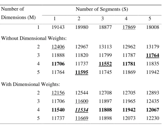
We estimate our AMDS model on the basis of the nested decision sets and dissimilarity judgments of the 212 subjects. To correct for differences in scale use, we first linearly transformed the dissimilarity judgments to having a minimum of 1 and a maximum of 7 for each individual subject, and preprocessed the individual data to achieve an average of 4 for each subject. As a result, the mean and variance of the dissimilarities are similar in size across subjects. We obtained estimates for two models: 1) the full model including all dimensional weights, and 2) a restricted model with the dimensional weights restricted to 1. Furthermore, to determine the most appropriate number of segments and dimensions, analyses have been performed for all combinations of S = 1,..,5 segments and M = 1,..,5 dimensions. Hence, in total 50 sets of parameter estimates are obtained for the AMDS model. We base model selection on the minimum CAIC criterion (see Table 4).
[ Insert Table 4 About Here ]
The “best” solution with dimensional weights, 2 segments, and 4 dimensions, yields the lowest CAIC value and is deemed most appropriate. The other model fit criteria generally indicate good to excellent model fit. The congruence coefficient CC for the dissimilarity data is very high: 0.920. For the nested set data, the overall average correct set membership probability is 0.784, and varies between 0.498 for VW, to 0.957 for Kia. The latent classes are reasonably well separated,
as indicated by the reduction of classification error RCE2 of 0.760 and the entropy statistic ES of 0.721. Furthermore, all model fit criteria improve only very slightly or not all if the number of segments or dimensions are increased which supports our model selection.
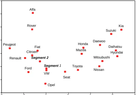
[ Insert Table 5 and Figure 1 About Here ]
Figure 1 and Table 5 contain the parameter values obtained with AMDS for S = 2 and M = 4. The perceptual map in Figure 1 shows the relative competitive positions of the twenty midsize car brands. Country-of-origin has a clear impact on the brand map, where the right-hand side of dimension 1 contains the Japanese and Korean brands and the left-hand side contains the European and American brands. For example, the French car brands (Renault, Peugeot and Citroën) and the Italian brand, Fiat, are tightly cluttered in the plot of the first two dimensions. To support interpretation of the dimensions, we correlate average attribute scores obtained for two familiar brands from each subject with each of the dimensions. The price, safety, sportiness, and design attributes have a significant negative correlation (p < 0.01) with the first dimension, namely –0.73, -0.67, -0.68, and -0.69). Hence, brands on the left-hand side are perceived as more expensive, safer, more sporty, and having a nicer design than brands on the right-hand side. Brands scoring low on dimension 2 are perceived as more long lasting (correlation is -0.54; p = 0.01), with the highest average ratings for durability for VW (5.33) and Opel (5.03). The attribute operation costs has a negative correlation with the third and fourth dimension, correlations being – 0.41 (p = 0.07) and –0.38 (p = 0.10) respectively. Furthermore, the reliability attribute correlates 0.37 (p = 0.10) with dimension 3. These perceptions match the higher reliability and lower repair costs which have indeed been reported for Toyota, Mazda and Nissan, whereas the opposite holds for Seat and Fiat (see for example AutoBild, TÜV Auto Report 2001).
Compared to the first two dimensions, the third and fourth dimension turn out to be harder to interpret, because they are less strong related to the attribute information available. Although such interpretation problems induce an additional burden for the researcher, it also constitutes an advantage over attribute-based perceptual mapping (Huber and Holbrook 1979) where the perceptual map is necessarily restricted to a pre-specified set of attributes. Interviews with industry experts could reveal the meaning of dimensions unrelated to the current set of attributes. If one succeeds in finding managerial relevant interpretations for these dimensions, the AMDS approach may reveal insights for product design and brand positioning which would not become apparent in an attribute-based perceptual mapping procedure.
Segments 1 and 2 comprise about two-third and one-third of the respondents, respectively (Table 5). For the brand dissimilarity perceptions, subjects from segment 2 weight the first dimension, reflecting country-of-origin, price and design, more heavily, whereas subjects from segment 1 weight the durability, reliability, and repair costs (dimensions 2 to 4) more heavily. The
set-related weights show that the fourth dimension is largely neglected by both segments while considering and choosing a brand. The ideal point of segment 1 is located very close to VW, and the ideal point of segment 2 is fairly close to the French car brands. The consideration set boundary is substantially wider for segment 2 than for segment 1. This points to larger consideration sets for consumers in segment 2 which is corroborated when we compute the set membership probabilities using equation 4 for each segment (Table 6). For segment 1, the consideration probability is negligible for most brands, whereas for segment 2 this probability is 10 to 20 percent even for brands located far from the segment ideal point. For example, Daihatsu is positioned far from both segment ideal points (Figure 1) but has nevertheless a probability of being considered of 13.1 percent in segment 2 and only 2.6 percent in segment 1. Contrary to the consideration set boundaries, the choice set boundaries are quite similar across the segments. Hence, differences in the brands being chosen are largely caused by the position of the segment ideal. For example, looking at Daihatsu again, the choice probabilities converged to 1.2 and 1.7 percent for segments 1 and 2, respectively. The top-3 brand choice probabilities for segment 1 are: VW (0.23), Opel (0.18), and Ford (0.08), and for segment 2: Renault (0.17), Citroën (0.13), and Peugeot (0.09), which emphasizes the important managerial differences between the two segments.
[ Insert Table 6 About Here ]
The proposed AMDS model assumes a single perceptual map to underlie both the brand dissimilarities and the nested decision sets. To check the validity of this model assumption, we additionally performed separate analyses for the dissimilarity data and the nested decision set data using the component model parts explained in the model section. The commonality in the parameters of these sub-models consists of the brand coordinates (the matrix X). Hence, we compared these two sets of estimates and those obtained analyzing the full data set. After Procrustes rotation of the perceptual maps, the proportion explained variance is extremely high, namely 98.5 percent. Hence, the three sets of brand coordinates are virtually the same. This is in line with our previous findings that consideration sets contain brands that are relatively similar and provides further support for the assumption that a single perceptual map is sufficient for representing both sets of data. Note, however, that all other model parameters depend on both of the two sets, so to obtain estimates for these both brand dissimilarities and nested decision sets are required.
VII. CONCLUSIONS
In this paper, we develop, test, and illustrate a new adaptive MDS (AMDS) procedure for mapping. The procedure deals with two important problems encountered in MDS research, namely the scaling of large brands sets and the problem with brand unfamiliarity. This is accomplished by adapting the data collection stage to the individual subject. The procedure uses a nested decision set framework for making brand choices: awareness, consideration, and choice. Information contained in the brand dissimilarities as well as in the nested decision sets is reflected in the derived estimates of the AMDS model. In the illustrative application to commercial data, adaptive MDS represented a complex data set comprising a large brand set by a parsimonious model with four dimensions and two segments. Importantly from a marketing perspective, the dimensions have a clear interpretation and the segments differed considerably in their choice behavior.
Our AMDS method builds upon four important developments in MDS research (Carroll and Green 1997). First, by making distributional assumptions on the data obtained, the model can be estimated in an ML framework and statistical tests can be performed on alternative specifications of the model. Second, by specifying a mixture model component, the method has the advantage of simultaneously obtaining segments of subjects and a perceptual map with brand coordinates and segment ideal points. Third, the AMDS method analyses multiple sets of variables simultaneously instead of sequentially. And fourth, we make use of developments in computer aided interviewing that allow the judgment task to be adapted on line to the individual respondent.
An important assumption of the joint representation of the consideration sets and the brand dissimilarities is that brands within a consideration set are relatively similar. The question on the similarity composition of consideration sets has been raised previously (Roberts and Lattin 1997), but has remained unanswered. We have shown that across a wide range of product categories that brands within a consideration set are indeed relatively similar, indicating that subjects focus, rather than broaden, their options at this stage. Further research should be done to assess effects of other moderator variables and using other samples of subjects, product categories, and brands.
In the application presented in this paper, we used a decompositional approach (Huber and Holbrook 1979) to perceptual mapping, because directly observed dissimilarity judgments were collected and analyzed. In a compositional approach, perceptions are studied via attribute ratings of brands. These attributes can be pre-specified or unrestricted and subject-specific
(Steenkamp, Van Trijp, and Ten Berge 1994). From both kinds of attribute ratings, however, dissimilarities between brands can be derived for each subject. In the compositional approach to positioning research, one may also restrict the data collection to a subject-specific subset of brands (Huber 1988) which may even be advisable since there too the number of judgments asked from subjects increases rapidly with the number of brands, quickly reaching the limit of what is feasible from the perspective of respondent burden. The AMDS model proposed in this paper can be applied to analyze the incomplete matrices of derived dissimilarities and can thus be applied to compositional data as well.
The adaptive data collection task, in which the set of brands is reduced sequentially, is based on the awareness, consideration, and choice set framework. The AMDS model can be applied also for alternative nested sets of brands assuming that dissimilarity judgments are made only for those brands in one of the smaller sets. One may also consider the sequence of brand sets as frequently used in advertising research: completely unfamiliar, aided recall, unaided recall, top-of-mind awareness. The nested structure could also be limited to familiar versus unfamiliar brands or pick-any choice data. Finally, an interesting area of application is decision making in business-to-business markets (Heide and Weiss 1995) where the final choice of suppliers is often made after specification of a short list and an even smaller set of firms invited to make a quotation. Applying the adaptive MDS model to such nested decision structures and similarities between competitors on the short lists would yield insights in the competitive structure between suppliers and a segmentation of industrial buyers.
Table 1. Analysis of Variance Assessing the Brand Similarity Composition of Consideration Sets.
Factor Sum of squares d.f. F-value p-value
Intercept Expertise Involvement Product category
Product category × Expertise Product category × Involvement
191.73 .08 .12 23.35 4.33 3.02 1 1 1 3 3 3 78.18 .03 .05 3.17 .59 .41 < .001 .860 .828 .026 .623 .746
Table 2. Average Relative Brand Similarity within Consideration Sets*
Product category
Compact cars Shower gel Radio stations Clothing shops
Expertise Low .82 1.71 0.97 .43 High 1.40 1.13 1.22 .47 Involvement High .75 1.57 1.01 .54 Low 1.45 1.24 1.17 .37 Total 1.13 1.41 1.10 .45
Table 3: Descriptive Statistics for the Automobile Brands
Percentage of respondents Percentage of respondents
Brand
Aware Consider Choice
Brand
Aware Consider Choice
Alfa Citroën Daewoo Daihatsu Fiat Ford Honda Hyundai Kia Mazda 80.2 92.0 74.1 67.5 93.4 98.1 92.5 78.8 38.7 85.4 4.2 20.3 9.4 3.8 8.5 14.6 13.2 9.0 0.5 13.7 1.4 10.4 3.8 0.5 3.3 6.1 2.4 2.8 0.0 4.2 Mitsubushi Nissan Opel Peugeot Renault Rover Seat Suzuki Toyota VW 88.7 90.1 99.5 96.4 91.5 65.1 82.5 80.7 92.5 99.1 9.4 10.8 31.1 17.0 26.9 8.0 7.5 5.2 20.8 37.3 1.4 2.8 18.4 2.8 11.3 1.9 2.8 0.9 6.1 16.5
Table 4: Model Fit (CAIC) for S = 1,..,5 and M =1,..,5∗
Number of Segments (S) Number of
Dimensions (M) 1 2 3 4 5
1 19143 18980 18877 17869 18008
Without Dimensional Weights: 2 3 4 5 12406 11888 11706 11764 12967 11820 11737 11595 13113 11799 11552 11745 12962 11787 11781 11869 13179 11764 11835 11942
With Dimensional Weights: 2 3 4 5 12156 11706 11540 11737 12544 11600 11534 11669 12708 11897 11808 11898 12705 11965 11942 12073 12893 12435 12067 12230
∗ Minimum values in each column (per model type) are indicated in boldface type, minimum values in each row are underlined, the best model overall (S=2, M=4, with weights) is indicated in italics.
Table 5: Parameter Estimates for Adaptive MDS Model with S = 2 and M = 4 Segments Parameters 1 2 Proportion λs .674 .33 Dissimilarity-weights Dimension 1 Dimension 2 Dimension 3 Dimension 4 ) (d sm w .825 1.059 1.057 1.004 1.175 .941 .943 .996 Set-weights Dimension 1 Dimension 2 Dimension 3 Dimension 4 ) (u sm w 1.251 1.162 1.268 .320 1.382 1.083 1.026 .509 Set Boundaries Choice Consideration cs b .637 .825 .533 1.407
Dissimilarity-related error dispersion σε .825 .965
Table 6. Predicted consideration and choice probabilities Segment 1 Segment 2 Brand Consideration probability Choice probability Consideration probability Choice probability Alfa Citroën Daewoo Daihatsu Fiat Ford Honda Hyundai Kia Mazda Mitsubushi Nissan Opel Peugeot Renault Rover Seat Suzuki Toyota VW .019 .076 .039 .026 .048 .138 .059 .027 .015 .100 .062 .071 .278 .083 .084 .036 .078 .021 .130 .338 .008 .040 .019 .012 .024 .081 .030 .012 .007 .055 .032 .037 .183 .045 .046 .017 .041 .010 .074 .232 .133 .448 .162 .131 .280 .237 .175 .122 .090 .273 .155 .183 .324 .370 .521 .174 .252 .120 .256 .273 .017 .128 .023 .017 .056 .043 .026 .015 .010 .054 .022 .028 .072 .091 .170 .026 .047 .015 .048 .054
Dimension 1 3 2 1 0 -1 -2 -3 D im e n s io n 2 4 3 2 1 0 -1 -2 -3 Segment 2 Segment 1 VW Toyota Suzuki Seat Rover Renault Peugeot Opel Nissan Mitsubushi Mazda Kia Hyundai Honda Ford Fiat Daihatsu Daewoo Citroen Alfa Dimension 3 3 2 1 0 -1 -2 -3 D im e n s io n 4 4 3 2 1 0 -1 -2 -3 Segment 2 Segment 1 VW Toyota Suzuki Seat Rover Renault Peugeot Opel Nissan Mitsubushi Mazda Kia Hyundai Honda Ford Fiat Daihatsu Daewoo Citroen Alfa
REFERENCES
Allenby, Greg M. and Peter E. Rossi (1999), “Marketing Models of Consumer Heterogeneity,” Journal of Econometrics, 89 (1-2), 57-78.
Andrews, Rick L., Asim Ansari, and Imran S. Currim (2002), “Hierarchical Bayes versus Finite Mixture Conjoint Analysis Models: A Comparison of Fit, Prediction, and Partworth Recovery,” Journal of Marketing Research, 39 (May), 87-98.
Bijmolt, Tammo H.A., Wayne S. DeSarbo, and Michel Wedel (1998), “A Multidimensional Scaling Model Accommodating Differential Brand Familiarity,” Multivariate Behavioral Research, 33 (1), 41-63.
Bijmolt, Tammo H.A. and Michel Wedel (1995), “The Effect of Alternative Methods of Collecting Similarity Data for Multidimensional Scaling,” International Journal of Research in Marketing, 12 (4), 363-371.
Bijmolt, Tammo H.A. and Michel Wedel (1999), “A Comparison of Multidimensional Scaling Methods for Perceptual Mapping,” Journal of Marketing Research, 36 (May), 277-285.
Bijmolt, Tammo H.A., Michel Wedel, Rik G.M. Pieters, and Wayne S. DeSarbo (1998), “Judgments of Brand Similarity,” International Journal of Research in Marketing, 15 (3), 249-268.
Borg, Ingwer and Detlev Leutner (1985), “Measuring Similarity of MDS Configurations,” Multivariate Behavioral Research, 20 (July), 325-334.
Bozdogan, Hamparsum (1987), “Model Selection and Akaike’s Information Criterion (AIC): The General Theory and its Analytical Extensions,” Psychometrika, 52 (September), 345-370.
Carroll, J. Douglas and Paul E. Green (1997), “Psychometric Methods in Marketing Research: Part II, Multidimensional Scaling,” Journal of Marketing Research, 34 (May), 193-204.
Chatterjee, Rabikar and Wayne S. DeSarbo (1992), “Accomodating Stimulus Unfamiliarity in the Multidimensional Scaling of Preference Data,” Marketing Letters, 3 (1), 85-99.
Cliff, N., R. Girard, R.S. Green, J.F. Kehoe, and L.M. Doherty (1977), “INTERSCAL: A TSO FORTRAN IV Program for Subject Computer Interactive Multidimensional Scaling,” Educational and Psychological Measurement, 37, 185-188.
Cooper, Lee G. (1983), “A Review of Multidimensional Scaling in Marketing Research,” Applied Psychological Measurement, 7 (Fall), 427-450.
Desai, Kalpesh K. and Wayne D. Hoyer (2000), “Descriptive Characteristics of Memory-Based Consideration Sets: Influence of Usage Occasion Frequency and Usage Location Familiarity,” Journal of Consumer Research, 27 (December), 309-323.
DeSarbo, Wayne S., Rabikar Chatterjee, Juyoung Kim (1994), “Deriving Ultrametric Tree Structures from Proximity Data Confounded by Differential Stimulus Familiarity,” Psychometrika, 59 (4), 527-566.
DeSarbo, Wayne S. and Kamel Jedidi (1995), “The Spatial Representation of Heterogeneous Consideration Sets,” Marketing Science, 14 (3, part 1), 326-342.
DeSarbo, Wayne S., Donald R. Lehmann, Gergory Carpenter, and Indrajit Sinha (1996), “A Stochastic Multidimensional Unfolding Approach for Representing Phased Decision Outcomes,” Psychometrika, 61 (3), 485-508.
DeSarbo, Wayne S., Ajay K. Manrai, and Lalita A. Manrai (1994), “Latent Class Multidimensional Scaling: An Review of Recent Developments in the Marketing and Psychometric Literature,” in: Advanced Methods of Marketing Research, Richard P. Bagozzi, ed. London: Blackwell, 190-222.
DeSarbo, Wayne S. and Jianan Wu (2001), “The Joint Spatial Representation of Multiple Variable Batteries Collected in Marketing Research,” Journal of Marketing Research, 38 (May), 244-253.
Green, Rex S. and Peter M. Bentler (1979), “Improving the Efficiency and Effectiveness of Interactively Selected MDS Data Designs,” Psychometrika, 44 (March), 115-119.
Hauser, John R. and Birger Wernerfelt (1990), “An Evaluation Cost Model of Consideration Sets,” Journal of Consumer Research, 16 (March), 393-408.
Heide, Jan B. and Allen M. Weiss (1995), “Vendor Consideration and Switching Behavior for Buyers in High Technology Markets,” Journal of Marketing, 59 (July), 30-43.
Huber, Joel (1988), “APM System for Adaptive Perceptual Mapping,” Journal of Marketing Research, 25 (February), 119-121.
Huber, Joel and Morris B. Holbrook (1979), “Using Attribute Ratings for Product Positioning: Some Distinctions among Compositional Approaches,” Journal of Marketing Research, 16 (November), 507-516.
Jobber, David and Ian G. Horgan (1988), “A Comparison of Techniques Used and Journals Taken by Marketing Researchers in Britain and the USA,” Service Industry Journal, 8 (3), 277-285.
Johnson, Michael D. and Elania J. Hudson (1996), “On the Perceived Usefulness of Scaling Techniques in Market Analysis,” Psychology & Marketing, 13 (7), 653-675.
Johnson, Michael D., Donald R. Lehmann, Claes Fornell, and Daniel R. Horne (1992), “Attribute Abstraction, Feature-Dimensionality, and the Scaling of Product Similarities,” International Journal of Research in Marketing, 9 (2), 131-147.
Johnson, Michael D., Donald R. Lehmann, and Daniel R. Horne (1990), “The Effects of Fatigue on Judgments of Interproduct Similarity,” International Journal of Research in Marketing, 7 (1), 35-43.