Applications and Advances in Similarity-based Machine Learning

(1)

UC Berkeley Electronic Theses and Dissertations

Permalink

https://escholarship.org/uc/item/6ch0g56s

Author

Spaen, Quico Pepijn

Publication Date

2019

Peer reviewed|Thesis/dissertation

eScholarship.org Powered by the California Digital Library

(2)

by

Quico Pepijn Spaen

A dissertation submitted in partial satisfaction of the requirements for the degree of

Doctor of Philosophy in

Engineering - Industrial Engineering and Operations Research in the

Graduate Division of the

University of California, Berkeley

Committee in charge:

Professor Dorit S Hochbaum, Chair Professor Alper Atamturk Assistant Professor Paul Grigas

Professor Satish Rao

(3)

(4)

Abstract

Applications and Advances in Similarity-based Machine Learning by

Quico Pepijn Spaen

Doctor of Philosophy in Engineering - Industrial Engineering and Operations Research University of California, Berkeley

Professor Dorit S Hochbaum, Chair

Similarity-based machine learning methods differ from traditional machine learning methods in that they also use pairwise similarity relations between objects to infer the labels of unlabeled objects. A recent comparative study for classification problems by Baumann et al. [2019] demonstrated that similarity-based techniques have superior performance and robustness when compared to well-established machine learning techniques. Similarity-based machine learning methods benefit from two advantages that could explain superior their performance: They can make use of the pairwise relations between unlabeled objects, and they are robust due to the transitive property of pairwise similarities.

A challenge for similarity-based machine learning methods on large datasets is that the number of pairwise similarity grows quadratically in the size of the dataset. For large datasets, it thus becomes practically impossible to compute all possible pairwise similarities. In 2016,

Hochbaum and Baumann proposed the technique of sparse computation to address this

growth by computing only those pairwise similarities that are relevant. Their proposed implementation of sparse computation is still difficult to scale to millions objects.

This dissertation focuses on advancing the practical implementations of sparse computation to larger datasets and on two applications for which similarity-based machine learning was particularly effective. The applications that are studied here are cell identification in calcium-imaging movies and detecting aberrant linking behavior in directed networks.

For sparse computation we present faster, geometric algorithms and a technique, named

sparse-reduced computation, that combines sparse computation with compression. The geometric algorithms compute the exact same output as the original implementation of sparse computation, but identify the relevant pairwise similarities faster by using the concept of data shifting for identifying objects in the same or neighboring blocks. Empirical results on datasets with up to 10 million objects show a significant reduction in running time. Sparse-reduced computation combines sparse computation with a technique for compressing highly-similar or identical objects, enabling the use of similarity-based machine learning on massively-large datasets. The computational results demonstrate that sparse-reduced computation provides a significant reduction in running time with a minute loss in accuracy.

(5)

A major problem facing neuroscientists today is cell identification in calcium-imaging movies. These movies are in-vivo recordings of thousands of neurons at cellular resolution. There is a great need for automated approaches to extract the activity of single neurons from these movies since manual post-processing takes tens of hours per dataset. We present the HNCcorr algorithm for cell identification in calcium-imaging movies. The name HNCcorr is derived from its use of the similarity-based Hochbaum’s Normalized Cut (HNC) model with pairwise similarities derived from correlation. In HNCcorr, the task of cell detection is approached as a clustering problem. HNCcorr utilizes HNC to detect cells in these movies as coherent clusters of pixels that are highly distinct from the remaining pixels. HNCcorr guarantees, unlike existing methodologies for cell identification, a globally optimal solution to the underlying optimization problem. Of independent interest is a novel method, named

similarity-squared, that we devised for measuring similarity between pixels. We provide an experimental study and demonstrate that HNCcorr is a top performer on the Neurofinder cell identification benchmark and that it improves over algorithms based on matrix factorization.

The second application is detecting aberrant agents, such as fake news sources or spam websites, based on their link behavior in networks. Across contexts, a distinguishing charac-teristic between normal and aberrant agents is that normal agents rarely link to aberrant ones. We refer to this phenomenon as aberrant linking behavior. We present an Markov Random Fields (MRF) formulation, with links as the pairwise similarities, that detects aberrant agents based on aberrant linking behavior and any prior information (if given). This MRF formulation is solved optimally and in polynomial time. We compare the optimal solution for the MRF formulation to well-known algorithms based on random walks. In our empirical experiment with twenty-three different datasets, the MRF method outperforms the other detection algorithms. This work represents the first use of optimization methods for detecting aberrant agents as well as the first time that MRF is applied to directed graphs.

(6)

List of Figures

2.1 Effect of sparse computation on accuracy. . . 8

2.2 Visualization of the block enumeration strategy. . . 11

2.3 Visualization of the object shifting strategy. . . 12

2.4 Visualization of the block shifting strategy. . . 14

2.5 Average running times for sparse computation algorithms . . . 18

2.6 Duplication ratio for sparse computation with data shifting. . . 19

2.7 Dimensional scaling for sparse computation algorithms. . . 20

2.8 Data-reduction step in Sparse-Reduced Computation . . . 21

3.1 Construction of auxiliary graph for linearized HNC. . . 36

3.2 Example of Sparse Computation for HNCcorr . . . 41

3.3 Visualization of correlation images of six pixels . . . 43

3.4 Percentage of active cells by dataset. . . 48

3.5 Cell identification results for datasets with active cells. . . 51

3.6 Contours of identified cells for two datasets. . . 51

3.7 Cell identification results for leading Neurofinder submissions. . . 53

(9)

List of Tables

2.1 Notation . . . 9

2.2 Dataset statistics. . . 15

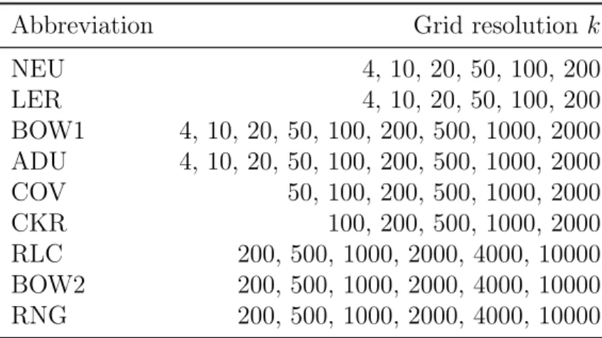
2.3 Reported grid resolutions. . . 17

2.4 Average runtime vs. grid resolution. . . 18

2.5 Dataset statistics . . . 24

2.6 Comparison of sparse and sparse-reduced computation for dataset COV. . . 26

2.7 Comparison of sparse and sparse-reduced computation for dataset KDD. . . 26

2.8 Comparison of sparse and sparse-reduced computation for dataset RLC. . . 27

2.9 Comparison of sparse and sparse-reduced computation for dataset BOW2. . . . 27

2.10 Comparison of sparse and sparse-reduced computation for dataset RNG. . . 27

3.1 Dataset characteristics . . . 47

3.2 Dataset-dependent parameter values for HNCccor by dataset. . . 50

4.1 Complexity of Markov Random Fields (MRF) problems. . . 59

4.2 Dataset characteristics. . . 66

4.3 Modularity performance by algorithm. . . 68

(10)

Acknowledgments

This work and the completion of my PhD would not have been possible without the support of numerous people. In particular, I would like to thank:

My parents, Frank Spaen and Jolande IJsseldijk, for guiding me to find my own path in life, giving me the freedom to move to another continent, and for their unwavering support for me; My girlfriend Aisling Scott for spicing up my life with fun over the past two years, her advice on numerous topics, and for believing in me; My brother and sister Joep and Floor Spaen for being the best brother and sister ever and for annihilating me at board games.

My advisor Dorit S. Hochbaum for her guidance, wisdom, and for believing in me. I really appreciate the countless hours we spent to discuss, analyze, and strategize for our research and teaching followed by extensive conversations about the most diverse and unrelated topics. We sometimes disagreed but our discussions were productive and always resulted in a better outcome.

My main co-authors, Roberto As´ın Ach´a, Philipp Baumann, Christopher Thraves Caro, and Mark Velednitsky, for our fruitful and enjoyable collaborations; Professors Alper Atamturk, Paul Grigas, Hillel Adesnik, and Satish Rao for their willingness to serve on my committee; The IEOR department staff, Keith McAleer, Diana Salazar, James Percy, Anayancy Paz, and Rebecca Pauling, for their support, helping me with questions I had, and for their positive energy; Professor Rhonda Righter for her care and interest in the well-being of students in the department.

My roommates Jian (Sam) Ju, Rob Clarke, and Valence Li for making me feel at home and for our many late-night conversations; My friend and fellow PhD student Amber Richter for our near-daily lunches and for introducing me to Aisling; My friends from the GPC Tuesday ride for sharing my joy in cycling and for keeping me healthy; Sheila Satin and friends for organizing so many fun social activities.

I would also like to thank all my fellow PhD students for our friendships, bar nights, Lunch & Learns, good advice, and many fun conversations. My thanks go to: Erik Bertelli, Clay Campaigne, Haoyang Cao, Junyu Cao, Ying Cao, Chen Chen, Carlos Deck, Shiman Ding, Yuhao Ding, Ilgin Dogan, Pelagie Elimbi Moudio, Salar Fattahi, Han Feng, Hao Fu, Andrés Gómez, Dean Grosbard, Tu˘g¸ce Gürek, Pedro Hespanhol, Anran Hu, Arman Jabbari, Titouan Jehl, Hansheng Jiang, Yusuke Kikuchi, Heejung Kim, Jiung Lee, Kevin Li, Tianyi Lin, Paula Lipka, Heyuan Liu, Sheng Liu, Stewart Liu, Alfonso Lobos, Cheng Lu, Yonatan Mintz, Igor Molybog, Julie Mulvaney-Kemp, Matt Olfat, Sangwoo Park, Georgios Patsakis, Meng Qi, Wei Qi, Xu Rao, Amber Richter, Rebecca Sarto Basso, Jiaying Shi, Auyon Siddiq, Birce Tezel, Mark Velednitsky, Renyuan Xu, Nan Yang, Min Zhao, Mo Zhou, Ruijie Zhou, and many others. Finally, I would like to thank all my other Berkeley friends and my fellow Graduate Assembly (GA) participants.

(11)

Chapter 1 Introduction

In supervised learning, the goal is to predict the label of an object based on the object’s feature vector. Most traditional machine learning methods approach this task by learning a function from a labeled training dataset that maps a feature vector to a label. This function is then applied to decide labels for unlabeled objects. A less common approach is to infer the labels of unlabeled objects based on pairwise similarity relations between all objects in the dataset, including those that are unlabeled, in addition to feature vectors. We refer to this approach as similarity-based machine learning.

There is mounting evidence that adding pairwise similarities considerably enhances the quality of pattern recognition and data mining techniques. This was demonstrated in a recent comparative study of fourteen different supervised learning techniques across twenty different datasets [Baumann et al., 2019]. In this study, similarity-based machine learning methods provided superior performance, as measured by F1-score, relative to non-similarity-based methods for classification problems. Similar observations have been made previously for classification problems [Dembczy´nski et al., 2009], medical diagnosis [Ryu et al., 2004], and for semi-supervised learning [Zhu et al., 2003].

A major advantage for similarity-based algorithms is that they benefit from a transitivity property. Distantly-similar objects can be labeled or grouped together due to a transitive chain of similarities [Kawaji et al., 2004]. The transitivity property also provides similarity-based algorithms with robustness, since similarity between a pair of objects is not only measured by comparing the two objects directly but also via multiple other paths of pairwise similarities via intermediate objects.

Another advantage for certain similarity-based machine learning methods is that they make use of the pairwise relations between unlabeled objects such as those in the test dataset. There are two similarity-based machine learning algorithms, Hochbaum’s Normalized Cut (HNC) [Hochbaum, 2010, 2013b] and Markov Random Fields (MRF) [Geman and Geman, 1984; Hochbaum, 2001], that have this unique feature. Other similarity-based machine learning algorithms, such as the k-Nearest Neighbors algorithm [Fix and Hodges, 1951] that classifies an object based on the labels of its k closest neighbors, are limited to pairwise similarities relations between labeled and unlabeled objects. Empirical evidence by Tresp

(12)

[2000] indicates that the performance of a method can improve by considering the relation between unlabeled objects. In his study, the performance of his ensemble method, the Bayesian Committee Machine (BCM), improved when considering multiple test objects simultaneously. This occurred because the BCM utilized the covariance between the test objects.

There are two primary reasons as to why similarity-based machine learning models are rarely used in practice. The first reason is the perceived lack of efficient machine learning techniques for dealing with pairwise similarities. However, efficient algorithms exist for e.g. both the HNC and MRF models [Ahuja et al., 2003, 2004; Hochbaum, 2001, 2010, 2013a]. The second concern is that it becomes practically impossible to compute all pairwise similarities for a large dataset, since the number of pairwise similarities grows quadratically in the size of the dataset. Hochbaum and Baumann [2016] introduced the method of sparse computation

to mitigate this problem.

This dissertation focuses on advancing the practical implementations of sparse computation and on two applications for which similarity-based machine learning was particularly effective. These applications are: Cell detection in calcium-imaging movies and detecting aberrant agents in networks based on link behavior. We now provide a brief description of the similarity-based models HNC and MRF that were used in these applications. Subsequently, we discuss the method of sparse computation for mitigating the quadratic growth in the number of pairwise similarities and two extensions for larger datasets. We then introduce the two applications in more detail.

1.1 Models for Similarity-Based Machine Learning:

Hochbaum’s Normalized Cut and Markov

Random Fields

Two models for similarity-based machine learning are Hochbaum’s Normalized Cut (HNC) [Hochbaum, 2010, 2013b] and Markov Random Fields (MRF) [Geman and Geman, 1984; Hochbaum, 2001, 2013a]. Both the HNC model and the MRF model with convex penalties are solved to global optimality in polynomial time with combinatorial algorithms [Ahuja et al., 2003, 2004; Hochbaum, 2001, 2010, 2013a].

Hochbaum’s Normalized Cut (HNC)

The clustering model Hochbaum’s Normalized Cut (HNC) [Hochbaum, 2010, 2013b] is a variant of the Normalized Cut problem for image segmentation that was popularized by Shi and Malik [2000]. The HNC model is defined on graph where nodes represent objects and edges are pairwise similarity relations. The model provides a trade-off between two objectives: High similarity between the objects in the cluster (homogeneity), and low similarity between objects in the cluster and the remaining objects (distinctness). The trade-off between the

(13)

two objectives is represented as either a ratio or a weighted linear combination. In either form, the model is polynomial time solvable [Hochbaum, 2010, 2013b] with combinatorial algorithms. In contrast, the Normalized Cut problem is known to be NP-Hard [Shi and Malik, 2000].

HNC is applicable to both supervised and unsupervised problems, and it has been successfully used across different contexts. These include image segmentation [Hochbaum et al., 2013], evaluating the effectiveness of drugs [Hochbaum et al., 2012], the detection of special nuclear materials [Yang et al., 2013], tracking moving objects in videos [Fishbain et al., 2013], and a comparative study on classification problems by Baumann et al. [2019]. In this study, it was demonstrated that the supervised variants of HNC (SNC & K-SNC) have the best overall performance and were the most robust among all algorithms considered, which included state-of-the-art machine learning techniques. Hochbaum et al. [2012]; Yang et al. [2013] also provide similar but less comprehensive comparisons between machine learning methods for drug ranking and the detection of special nuclear materials. These experiments also indicated that SNC was among the top performing machine learning methods for these contexts.

Markov Random Fields Problem (MRF)

The Markov Random Fields (MRF) [Geman and Geman, 1984; Hochbaum, 2001, 2013a; Kleinberg and Tardos, 2002] was originally considered in image segmentation, where pixels from a noisy image should be assigned to a set of colors. Similar to the HNC model, the objective in the MRF model also presents a trade-off. The trade-off for the MRF model is between two types of similarities: The similarity between an object and its prior and the pairwise similarity between pairs of objects. Each type has an associated penalty in the objective function: A deviation penalty for when the assigned value of an object deviates away from a prior value, and a separation penalty for when the assigned values of a pair of objects differ. In image segmentation, the deviation penalties penalizes deviations with respect to the original color of the pixel whereas the separation penalties smooth the colors assigned to adjacent pixels. When the separation penalty functions are convex, the MRF problem is solved optimally and efficiently in either continuous or integer variables [Ahuja et al., 2003, 2004; Hochbaum, 2001]. The problem is NP-hard otherwise [Hochbaum, 2001]. Aside from image segmentation [Hochbaum, 2001, 2013a; Qranfal et al., 2011], MRF has been applied successfully for group decision-making [Hochbaum and Levin, 2006], rating customers’ propensity to buy new products [Hochbaum et al., 2011], ranking the credit risk of countries [Hochbaum and Moreno-Centeno, 2008], and for yield prediction in semiconductor manufacturing [Hochbaum and Liu, 2018]. In all of these applications, the separation penalties were defined on undirected graphs. The MRF application presented below is unique in that the separation penalties are directional and are defined on a directed graph. The algorithms listed above apply to both types of graphs.

(14)

1.2 Sparse Computation for Mitigating the Quadratic

Growth of Similarities

A challenge for similarity-based machine learning methods on large datasets is that the number of pairwise similarity grows quadratically in the size of the dataset. For large datasets, it thus becomes practically impossible to compute all possible pairwise similarities.

Hochbaum and Baumann [2016] proposed the technique of sparse computation to address this growth by computing only those pairwise similarities that are relevant. Sparse com-putation enables the scaling of similarity-based algorithms to large datasets. The method first project the objects’ feature vectors into a low-dimension space. This is commonly done with the dimension reduction method approximate principle component analysis, a variant of principle component analysis (PCA). Sparse computation uses closeness of two objects in the low-dimensional space as a proxy for the relevance of the associated pairwise similarity. To identify close pairs of objects in the low-dimensional space, the low-dimensional space is discretized into grid blocks. A pair of objects is considered relevant if the objects belong to the same or adjacent grid blocks. The pairwise similarities are then computed for all relevant pairs with the original feature vectors.

The Hochbaum and Baumann [2016] implementation of sparse computation is still difficult to scale to millions objects. We present in this work two extensions that scale the method of sparse computation to very-large datasets (see also [Baumann et al., 2016, 2017]).

The first extension consists of faster geometric algorithms for sparse computation. These geometric algorithms compute the exact same output as the original implementation of sparse computation, but identify the relevant pairwise similarities faster by using the concept of

data shifting for identifying objects in the same or neighboring blocks. Empirical results on datasets with up to 10 million objects show a significant reduction in running time. The new algorithms also result in improved scaling for sparse computation with respect to the dimension of the low-dimensional space.

The second extension is the technique of sparse-reduced computation. Sparse-reduced computation combines sparse computation with a technique for compressing highly-similar or identical objects, enabling the use of similarity-based machine learning on massively-large datasets. Due to the compression, sparse-reduced computation provides a different output than sparse computation and replaces groups of objects by new representative objects. The computational results demonstrate that sparse-reduced computation provides very similar accuracy as sparse computation with a significant reduction in runtime. Sparse-reduced computation allows for highly-accurate classification of datasets with millions of objects in seconds.

(15)

1.3 Applications: Cell Identification in Neuroscience

and Aberrant Agent Detection in Networks with

Similarity-based Machine Learning

A major problem facing neuroscientists today is detecting cells in calcium-imaging movies. Calcium imaging is a modern technique used by neuroscientists for recording movies of in-vivo neuronal activity at cellular resolution. Using genetically encoded calcium indicators and fast laser-scanning microscopes, it is now possible to record thousands of neurons simultaneously. However, the manual post-processing needed to extract the activity of single neurons requires tens of hours per dataset. Consequently, there is a great need to develop automated approaches for the extraction of neuronal activity from imaging movies.

We present a similarity-based algorithm, named HNCcorr, for cell detection in calcium imaging movies (see also [As´ın-Ach´a et al., 2019; Spaen et al., 2019]). The name HNCcorr is derived from the use of HNC and that of pairwise similarities based on correlation. In HNCcorr, the task of cell detection in calcium imaging movies is approached as a clustering problem. HNCcorr utilizes HNC to detect cells in these movies as coherent clusters of pixels that are highly distinct from the remaining pixels. HNCcorr guarantees, unlike existing methodologies for cell identification, a globally optimal solution to the underlying optimization problem. Of independent interest is a novel method, namedsimilarity-squared, that we devised for measuring similarity between pixels. We provide an experimental study and demonstrate that HNCcorr is a top performer on the Neurofinder cell identification benchmark and that it improves over algorithms based on matrix factorization [Pachitariu et al., 2017; Pnevmatikakis et al., 2016]. This algorithm represents the first use of similarity-based machine learning methods in neuroscience.

The second application is detecting aberrant agents in networks based on their link behavior. Agents with aberrant behavior are commonplace in today’s networks; there are fake profiles in social media, spam websites on the internet, and fake news sources that are prolific in spreading misinformation. The viral spread of digital misinformation has become so severe that the World Economic Forum considers it among the main threats to human society [World Economic Forum, 2013]. It is thus crucially important to be able to identify aberrant agents. Across contexts, a distinguishing characteristic between normal and aberrant agents is that normal agents rarely link to aberrant ones. We refer to this phenomenon as

aberrant linking behavior.

We present an MRF formulation that detects aberrant agents based on the link behavior of agents in the network. The formulation balances two objectives: to satisfy aberrant linking behavior by having as few links as possible from normal to aberrant agents, as well as to deviate minimally from prior information (if given). The MRF formulation is solved optimally and efficiently. We compare the optimal solution for the MRF formulation to well-known algorithms based on random walks [Rajaraman and Ullman, 2011], including PageRank [Page et al., 1999], TrustRank [Gy¨ongyi et al., 2004], and AntiTrustRank [Krishnan and Raj, 2006]. To assess the performance of the algorithms, we present a variant of the modularity clustering

(16)

metric that overcomes the known shortcomings of modularity in directed graphs. We show that this new metric has desirable properties and prove that optimizing it is NP-hard. In our empirical experiment with twenty-three different datasets, the MRF method outperforms the other detection algorithms. This work is the first use of optimization methods for detecting aberrant agents as well as the first time that MRF is applied with directed links.

1.4 Overview of this Dissertation

Chapter 2 presents the improved methodologies for sparse computation. The chapter starts with an overview of the sparse computation method. Then, the geometric algorithms for sparse computation are presented, and their performance is analyzed in a computational study. Subsequently, the sparse-reduced computation method is presented. Sparse-reduced computation extends sparse computation by adding compression of highly-similar objects. An experimental study of its performance relative to sparse computation is provided.

Chapter 3 introduces the HNCcorr algorithm for cell detection in calcium imaging. The chapter includes a discussion of the HNC model and algorithms for solving it. The HNCcorr algorithm is described, and a discussion of how it incorporates HNC and sparse computation is provided. Having described the algorithm, the chapter concludes with an experimental comparison between HNCcorr and other cell identification algorithms.

Chapter 4 lays out our approach for detecting aberrant agents in directed networks based on their linking behavior with MRF. The chapter provides the general MRF model, algorithms for solving it, and our MRF formulation for the detection of aberrant agents. The experimental performance of MRF is compared with other well-known algorithms.

(17)

Chapter 2 Improved Methodologies for Sparse

Computation: Geometric Algorithms

and Sparse-Reduced Computation

Computing pairwise similarities poses a challenge in terms of scalability as the number of pairwise similarities between objects grows quadratically in the number of objects in the dataset. For large datasets, it is prohibitive to compute and store all pairwise similarities.

Various methods have been proposed that sparsify a complete similarity matrix, which contains all pairwise similarities, while preserving specific matrix properties [Arora et al., 2006; Jhurani, 2013; Spielman and Teng, 2011]. A sparse similarity matrix requires less memory and allows faster classification as the running time of the algorithms depends on the number of non-zero entries in the similarity matrix. These approaches are not suitable for large-scale datasets because they require as input the complete similarity matrix.

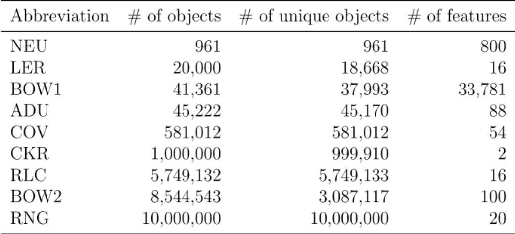
Recently, Hochbaum and Baumann [2016] introduced a methodology called sparse com-putation that generates a sparse similarity matrix without having to compute the complete similarity matrix first. Sparse computation enables the scaling of similarity-based machine learning methods to large dataset by significantly reducing the running time of the classifiers without affecting their accuracy (see Figure 2.1). In sparse computation the data is efficiently projected onto a low-dimensional space using a probabilistic variant of principal component analysis. The low-dimensional space is then subdivided into grid blocks and pairwise simi-larities are only computed between objects in the same or in neighboring grid blocks. The density of the similarity matrix can be controlled by varying the grid resolution. A higher grid resolution leads to a sparser similarity matrix. In section 2.1, we review the sparse computation technique in more detail.

For large-scale datasets, the computational bottleneck of sparse computation is the identification of pairs of adjacent blocks in the grid structure. For each non-empty block, it identifies adjacent blocks and checks whether these blocks are non-empty. This process is referred to as block enumeration. For large-scale datasets to which sparse computation is applied with a high grid resolution, the vast majority of adjacent blocks are empty, but are

(18)

98 95 90 50 0 Degree of sparsity (%) 90.0 92.5 95.0 97.5 100.0 T est Accuracy (%) KNN SNC SVM

Figure 2.1: Accuracy at selected sparsity levels for the letter recognition (LER) dataset obtained with three similarity-based classifiers - k-nearest neighbors, SNC [Hochbaum, 2010], and SVM [Cortes and Vapnik, 1995] - on a sparse similarity matrix generated with sparse computation. Sparsity, reported on a log scale, is measured as the percentage of matrix entries that are not computed. The runtime of the algorithms is inversely proportional to the sparsity of the similarity matrix.

still checked. Hence, a large fraction of the computational workload is unnecessary.

In section 2.2, we present two new algorithms for sparse computation that address this computational bottleneck. The algorithms are based on a computational geometry concept called data shifting, which is used to identify pairs of similar objects in a low-dimensional space much faster than with state-of-the-art techniques.

Computational experiments in section 2.3 demonstrate that the new algorithms for sparse computation are up to five times faster. The improved algorithms enable the scaling of sparse computation to datasets with millions of objects. Furthermore, the new algorithms improve the scaling of sparse computation with respect to the dimension of the low-dimensional space.

Regardless of which sparse computation algorithm is applied, it may occur that large groups of highly-similar or identical objects project to the same grid block even when the grid resolution is high. As a result, a large number of pairwise similarities between nearly-identical objects is identified by sparse computation. The computation of similarities between these objects is unnecessary as they often belong to the same class. In massively-large datasets, large numbers of highly-similar objects are particularly common. The grid block structure created in sparse computation reveals the existence of such highly-similar objects in the dataset.

In section 2.4, we propose an extension of sparse computation called sparse-reduced computation that avoids the computation of similarities between highly-similar and identical objects through compression. The method builds on sparse computation by using the grid block structure to identify highly-similar and identical objects efficiently. In each grid block, the objects are replaced by a small number of representatives. The similarities are then computed only between representatives in the same and in neighboring blocks. The resulting similarity matrix is not only sparse but also smaller in size due to the consolidation of objects.

(19)

Table 2.1: Notation

Symbol Description

n Number of objects

d Number of features

x1, . . . ,xn∈Rd Objects - represented by their feature vectors

p Number of dimensions in low-dimensional space

k and k0 Grid resolution

κ Sub-block grid resolution in sparse-reduced computation

ω Pre-specified L∞ distance

datasets containing up to 10 million objects in section 2.5. Sparse-reduced computation delivers highly-accurate classification at very low computational cost for most of the studied datasets.

Throughout this chapter, we use the notation given in Table 2.1.

2.1 Overview of Sparse Computation

Sparse computation [Hochbaum and Baumann, 2016] takes as input a dataset with n objects x1, . . . ,xn ∈Rd andd features. The method consists of the steps: dimension reduction, grid

construction and selection of pairs, and similarity computation.

In the dimension reduction step, the input data is projected from a d-dimensional space onto a p-dimensional space, where pd. The projection is done with a probabilistic variant of PCA called approximate PCA [Hochbaum and Baumann, 2016]. Let the data in the

p-dimensional space be normalized, i.e., the values of each dimension are scaled to the range [0,1].

In the grid construction and selection of pairs step, the goal is to select all pairs of objects that have an L∞ distance smaller or equal to ω in the p-dimensional space. This is achieved

as follows. First, the range of values along each dimension is subdivided into k= _ω1 equally long intervals. This partitions the p-dimensional space into kp _{grid blocks. Parameter} _k

denotes the grid resolution. Each object is then assigned to a single block based on its p

coordinates. Objects which lie exactly on a grid line (horizontally and/or vertically) are assigned to the upper and/or right grid block. If the upper and/or right grid block is outside the grid, then the object is assigned to the lower and/or left block.

Since the largest L∞ distance within a block is equal to ω = _k1, all pairs of objects that

belong to the same block are selected. In addition, some pairs of objects are within a distance of ω but fall in different blocks. To select those pairs as well, horizontally, vertically, and diagonally adjacent blocks need to be considered. Each block has up to 3p₋_{1 neighbors. We}

refer to this process as block enumeration. By selecting all pairs of objects that are assigned to adjacent blocks, it can be guaranteed that all pairs of objects whose distance is less than

(20)

or equal to ω are selected. It is possible that pairs of objects whoseL∞ distance is more than ω but less than 2ω are selected as well, whereas objects whose distance is more than 2ω will not be selected.

The total number of selected pairs depends on the grid resolution k and the dimension of the low-dimensional space p. A higher grid resolution results in smaller blocks and thus reduces the set of pairs that fall in a block or its adjacent blocks. Similarly, when the number of dimensions of the low-dimensional space is increasing, the blocks contain fewer objects and this reduces the number of pairs selected.

In the similarity computation step, a similarity function is used to quantify the similarity for each of the pairs selected in the previous step. The similarity value is computed with respect to the original d-dimensional space.

The selection of pairs in sparse computation relies on enumerating (3p₋₁₎_/_{2 adjacent}

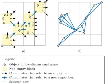
blocks for each non-empty block to determine pairs of adjacent non-empty blocks1. This computation becomes the bottleneck of the method when a) the number of non-empty blocks is large, and b) most of the adjacent blocks are empty. Checking empty blocks is unnecessary and only contributes to the runtime. Conditions a) and b) are often met when sparse computation is applied with high grid resolution to a large-scale dataset with millions of objects. To illustrate this issue, Figure 2.2 shows a two-dimensional projection of a dataset that contains 12 objects. With a grid resolution of k = 4, the two-dimensional space was partitioned into 16 blocks, six of which are non-empty. To find the adjacent blocks of the six non-empty blocks, 24 other blocks (visualized by arrows) are considered. Only 6 out of these 24 blocks are non-empty (blue arrows). The plot on the right hand side of Figure 2.2 highlights all selected pairs by blue lines that connect the corresponding objects.

2.2 Geometric Algorithms for Sparse Computation

To address the bottleneck of identifying pairs in adjacent blocks, we introduce a computational geometry concept called data shifting. We show how data shifting can be used to devise two geometric algorithms for sparse computation: object shifting andblock shifting. These algorithms replace the block enumeration process in the second step of sparse computation. The object shifting algorithm shifts the objects multiple times along different directions within the grid structure. For each shift, the pairs of objects that fall in the same block are deemed to be similar. Object shifting avoids having to explicitly compute adjacent blocks, but the same pair of objects may be selected for multiple shifts. We refer to such pairs as

duplicate pairs. The block shifting algorithm partially addresses the drawback of duplicate pairs by identifying all pairs of non-empty adjacent blocks by shifting representatives for non-empty blocks instead of the individual objects. Note that these two algorithms generate the exact same set of pairs as sparse computation with block enumeration.

1_{For each non-empty block, only half of the adjacent blocks need to be checked since the adjacency}

(21)

a) b) Legend:

Object in low-dimensional space Non-empty block

Coordinates that refer to an empty box Coordinates that refer to a non-empty box Selected pair

Figure 2.2: Visualization of the block enumeration strategy withk = 4 andp= 2: a) for each non-empty block, four adjacent blocks must be considered to identify all pairs of adjacent non-empty blocks. The majority of considered blocks are empty (dotted arrows). b) all pairs of objects that fall into the same or in neighboring blocks are selected (blue lines)

The concept of data shifting

Sparse computation relies on a grid to identify close pairs of objects in the low-dimensional space. The identified pairs are all within an L∞ distance of ω and potentially some within

an L∞ distance of 2ω. In contrast to sparse computation with block enumeration, the

low-dimensional space is partitioned into k0p grid blocks fork0 = ₂1_ω. Each grid block is thus twice as large in each dimension. All objects within a grid block are now within an L∞

distance of 2ω. The grid, however, might still arbitrarily separate objects that are close by a grid line. Two objects that are within an L∞ distance ofω, but separated by a grid line,

are denoted as border pair. In a two-dimensional grid, there are three types of border pairs: horizontal border pairs, vertical border pairs, and diagonal border pairs. In a p-dimensional grid, there are 2p−1 types of border pairs. Data shifting addresses the issue of identifying border pairs by shifting the data from its initial position along a single or multiple axes such that all border pairs of one type will no longer be separated by a grid line after the shift. To capture all types of border pairs, 2p−1 shifts are required. In each shift, the data is shifted byω along the respective axes. This is sufficient to identify all close neighbors of an object, since for each neighbor that is within a distance of ω from the object there exist at least one grid such that they belong to the same grid block. By efficiently identifying all close neighbors, data shifting provides a 2-approximation for the problem of identifying, for each object, the set of neighbors that are within an L∞ distance of ω.

(22)

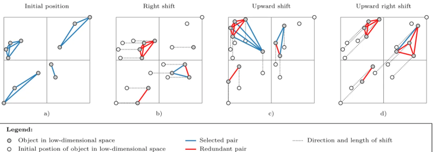
Initial position a) Right shift b) Upward shift c)

Upward right shift

d) Legend:

Object in low-dimensional space

Initial postion of object in low-dimensional space

Direction and length of shift Selected pair

Redundant pair

Figure 2.3: Visualization of the object shifting algorithm with grid resolution k0 = 2 for a dataset projected to a p= 2 dimensional space: a) selection of pairs of objects that fall in the same grid block, b) objects are horizontally shifted by 1/k to capture horizontal border pairs. c) objects are vertically shifted by 1/k to capture vertical border pairs, d) objects are diagonally shifted to capture diagonal border pairs. Redundant pairs are highlighted in red.

Object shifting algorithm

To get exactly the same selection of similar pairs as the block enumeration strategy with a grid resolution of k, the object shifting algorithm first partitions the low-dimensional space into k0p _{grid blocks for} _k0 ₌ 1

2k . Based on the concept of data shifting, 2

p₋_{1 directions are}

determined. Given p, the directions can be determined by generating binary representations of width p of the integers [1, . . ., 2p −1]. Each bit corresponds to a dimension and a one means that the data is shifted along this dimension. For example, if p = 2, the binary representations are 01, 10, and 11. The algorithm is called object shifting because all objects are shifted by _k1 = ₂1_k0 in that direction. Based on the new coordinates, each object is assigned

to a single grid block and all pairs of objects that are assigned to the same block are selected. Since the same pairs of objects might be assigned to the same block in different shifts, one needs to identify and remove duplicate pairs. If the grid resolution is high and hence the total number of selected pairs is low, the runtime for identifying and removing redundant pairs is negligible. However, if the grid resolution is low and the total number of selected pairs is large, then identifying and removing redundant pairs can become computationally expensive. Figure 2.3 illustrates object shifting algorithm for our two-dimensional example. The original position of the data is shown in the top left plot.

Block shifting

The disadvantage of object shifting is that certain pairs are selected for multiple shifts. In particular, objects that fall in the same sub-block, defined by splitting the blocks in half in

(23)

each dimension, will fall in the same block for each shift and are thus repeated 2p−1 times. Block shifting addresses this by replacing them with a single object.

To generate the same pairs as sparse computation with block enumeration with grid resolution k, thep-dimensional space is first partitioned with a grid resolution of k into kp

grid blocks and each object is assigned to the corresponding block. The corresponding pairs for each block are selected. Instead of identifying the border pairs directly with data shifting each non-empty block is first replaced with a representative object at its center. Note that this new dataset consists of objects that are located at multiples of ₂1_k along the dimensions. All coordinates are within the range [₂1_k,1− 1

2k] and the L∞ distance between pairs of objects

that represent adjacent blocks is exactly 1_k. Hence, we can apply the object shifting algorithm to the new dataset with a grid resolution of k0 = 1₂k to find all pairs of adjacent blocks. Finally, all pairs of objects that consists of objects in adjacent blocks are selected. Figure 2.4 illustrates block shifting for our two-dimensional example.

Runtime analysis

The runtime of block enumeration, object shifting, and block shifting depends on the parameters k and pand on the distribution of the objects within the low-dimensional space. Since all algorithms have the same output, they only differ with respect to the overhead (unnecessary work performed): The object/block shifting algorithms may identify pairs of objects/representatives more than once, and the block enumeration algorithm may enumerate empty adjacent blocks.

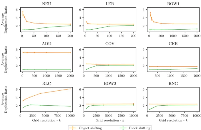
The overhead of the block enumeration is large when objects fall into many isolated blocks. This typically occurs for large k and p. The overhead of object shifting is large when many objects fall into few adjacent blocks. This typically occurs for small k and p. The overhead of block shifting is only large when the number of adjacent representatives is large. This does not occur for small or for large values of k and p. To obtain a large number of adjacent representatives, few objects must fall in a large number of adjacent blocks. Hence, the number of adjacent representatives tends to initially increase with increasingp andk, but decreases again once the blocks become isolated. In practice, we observe that block shifting identifies a pairwise similarity no more than twice. For more details, see the experimental results in section 2.3 and Figure 2.6.

2.3 Experimental Analysis of Geometric Algorithms

for Sparse Computation

We compared the runtime of block enumeration, object shifting, and block shifting for different grid resolutions on nine datasets. We evaluated only runtime because all algorithms generate the same output when the grid resolutions are chosen accordingly. Extensive empirical results on how sparse computation and thus the new algorithms affect the accuracy of (un)supervised learning algorithms are presented in [Baumann, 2016; Hochbaum and Baumann, 2016].

(24)

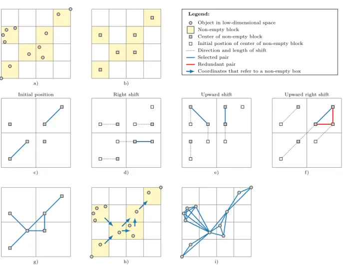
a) b) Initial position c) Right shift d) Upward shift e)

Upward right shift

f)

g) h) i)

Legend:

Object in low-dimensional space Non-empty block

Center of non-empty block

Initial postion of center of non-empty block Direction and length of shift

Selected pair Redundant pair

Coordinates that refer to a non-empty box

Figure 2.4: Visualization of the block shifting algorithm with grid resolution k = 4 for a dataset projected to a p= 2 dimensional space: a) low-dimensional space is partitioned with grid resolution k, b) each non-empty block is replaced by a representative, c)–f) the object shifting algorithm is applied with grid resolution k0 = 2 to find pairs of representatives that correspond to neighboring blocks (redundant pairs of representatives are highlighted in red), g)–i) the identified pairs of representatives are used to select pairs of objects that fall within the same or within neighboring blocks.

(25)

We implemented the algorithms and the computational analysis in Python 3.5. The source code is available athttps://github.com/hochbaumGroup/sparsecomputation. The source code of the computational analysis is available at https://github.com/quic0/sparse-experiments.

datasets

The datasets represent various domains including life sciences, engineering, social sciences and business and have sizes ranging from hundreds to millions of objects. Six real-world datasets were taken from the UC Irvine Machine Learning Repository [Lichman, 2013], two datasets were taken from previous studies [Breiman, 1996; Dong, Jian-xiong et al., 2005; Lee and Mangasarian, 2001; Tsang et al., 2005], and one real-world dataset was taken from the Neurofinder public benchmark for calcium imaging [CodeNeuro, 2017]. In all datasets, we substituted categorical features by a binary feature for each category and removed any duplicate objects. We briefly describe each dataset and mention further modifications that we made. Statistics about each of the datasets are provided in Table 2.2.

The dataset Adult (ADU) [Kohavi, 1996] stems from the census bureau database and each object represents a person. In the original dataset there is a categorical and a continuous feature to capture the educational level of the persons. To avoid double use, we removed the categorical feature. In addition, we removed all features that contain missing values.

In the Bag of Words dataset (BOW), the objects are documents from five different sources. The sources are Enron emails, KOS blog entries, New York Times articles, NIPS full papers, and PubMed abstracts. A document in this dataset is represented as a bag of words, i.e., a set of vocabulary words. This representation disregards word order but keeps word multiplicity. We generated two datasets from the bag of words dataset: BOW1 contains the NIPS full papers and the Enron emails. For each document in BOW1, we divide the number of occurrences of each word by the total number of words in the document to obtain the

Table 2.2: Statistics of the datasets (after modification) Abbreviation # of objects # of unique objects # of features

NEU 961 961 800 LER 20,000 18,668 16 BOW1 41,361 37,993 33,781 ADU 45,222 45,170 88 COV 581,012 581,012 54 CKR 1,000,000 999,910 2 RLC 5,749,132 5,749,133 16 BOW2 8,544,543 3,087,117 100 RNG 10,000,000 10,000,000 20

(26)

relative frequencies. BOW2 contains the New York Times articles and the PubMed abstracts. For BOW2, we limit the feature space to the 100 words with the largest absolute difference in mean relative frequency between the New York Times articles and the PubMed abstracts. A binary vector indicates which of those words occur in the respective document.

The datasetCheckerboard (CKR) is an artificial dataset that has been used for evaluating large-scale SVM implementations [Lee and Mangasarian, 2001; Tsang et al., 2005]. Each object represents a point on a 4×4 checkerboard that is characterized by two features which represent the x- and the y-coordinates. Following [Tsang et al., 2005], we create a checkerboard dataset with 1 million objects by randomly choosing the x- and y-coordinates of objects between -2 and 2 according to a uniform distribution.

The dataset Covertype (COV) [Blackard and Dean, 1999] contains cartographic character-istics of forest cells in northern Colorado. There are seven different cover types which are labeled 1 to 7.

The dataset Letter Recognition (LER) [Frey and Slate, 1991] comprises 20,000 objects. Each object corresponds to an image of a capital letter from the English alphabet.

The dataset Neuron (NEU) [CodeNeuro, 2017] is a calcium imaging recording of a neuron, a brain cell. The objects are the pixels in the recording and the features are the intensity of a pixel for each of the frames. Sparse computation is used as a subroutine in a leading algorithm for cell identification in calcium imaging recordings [Spaen et al., 2019].

In the dataset Record Linkage Comparison Patterns (RLC) [Schmidtmann et al., 2009], the objects are comparison patterns of pairs of patient records. We substitute the missing values with value zero and introduce a binary feature to indicate missing values. The objects can be classified as match or no-match.

The dataset Ringnorm (RNG) is an artificial dataset that has been used in [Breiman, 1996] and [Dong, Jian-xiong et al., 2005]. The objects are points in a 20-dimensional space and belong to one of two Gaussian distributions. Following the procedure of [Dong, Jian-xiong et al., 2005], we generate a Ringnorm dataset instance with 10 million objects.

Experimental design

We compared the runtime of sparse computation with block enumeration, object shifting, and block shifting on the nine datasets for different grid resolutions k. For large datasets, it was impossible to construct the complete similarity matrix due to memory limitations of our machine. The grid resolutions used for each of the datasets are described in Table 2.3. We chose the number of dimensions pof the low-dimensional space to be 3 for all datasets except for CKR for which we chose 2 because it only has two features. For the dimension reduction step, we used approximate PCA [Hochbaum and Baumann, 2016] which is much faster than exact PCA as it reduces the size of the original dataset by sampling a small fraction of objects and features. Here we set the sampling fraction for objects to one percent and the sampling fraction for features to five percent unless the number of features is less than 150 in which case all features were used. Only the NEU and BOW1 datasets have more than 150 features.

(27)

Table 2.3: Grid resolutions reported for each dataset

Abbreviation Grid resolution k

NEU 4, 10, 20, 50, 100, 200 LER 4, 10, 20, 50, 100, 200 BOW1 4, 10, 20, 50, 100, 200, 500, 1000, 2000 ADU 4, 10, 20, 50, 100, 200, 500, 1000, 2000 COV 50, 100, 200, 500, 1000, 2000 CKR 100, 200, 500, 1000, 2000 RLC 200, 500, 1000, 2000, 4000, 10000 BOW2 200, 500, 1000, 2000, 4000, 10000 RNG 200, 500, 1000, 2000, 4000, 10000

We ran each combination of algorithm, dataset, and grid resolution five times and recorded the mean runtime and the standard deviation across all five runs. In addition, we recorded various statistics that affect the runtime of the algorithms. The computational analysis was performed on a workstation with Intel Xeon CPUs (model E5-2667 v2) with clock speed 3.30 GHz and 256 GB of RAM.

Experimental results

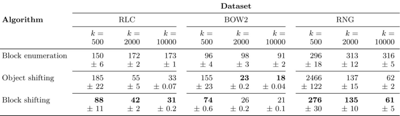
The mean and standard deviations of the runtimes of the different algorithms are reported in Figure 2.5 and for the largest three datasets in Table 2.4. Sparse computation with block enumeration performs well at low grid resolutions, but gets slow when applied with high grid resolutions. In contrast, sparse computation with object shifting performs poorly at low grid resolutions because there is a large number of pairs consisting of objects that fall into the same sub-block and are selected for each shift. Sparse computation with object shifting performs well when the grid resolution is high. At these grid resolutions, few objects fall in the same sub-block and fewer duplicate pairs are selected.

Sparse computation with block shifting combines the properties of sparse computation with block enumeration and object shifting and provides (near-) best runtime across datasets and grid resolutions. Although outperformed by object shifting at extremely high grid resolutions, it does not suffer from the pitfalls that affect block enumeration and object shifting. By replacing each sub-block by a single representative, it significantly reduces the number of duplicate pairs. This results in faster runtimes for low grid resolutions when each block typically contains multiple objects. Figure 2.6 shows that block shifting identifies only few duplicate pairs for low grid resolutions. For all datasets block shifting identifies, on average, a pair no more than twice independent of the grid resolution.

An interesting insight can be gained from the CKR dataset: although object shifting generates more duplicate pairs than block shifting, it is still slightly faster for very high grid resolutions. This is most likely due to the overhead resulting from generating the

(28)

0 50 100 150 200 10−1 100 Running time (s) NEU 0 50 100 150 200 100 102 LER 0 500 1000 1500 2000 102 103 BOW1 0 500 1000 1500 2000 101 103 Running time (s) ADU 0 500 1000 1500 2000 101 102 COV 500 1000 1500 2000 101 102 CKR 0 2500 5000 7500 10000 Grid resolution -k 103 102 Running time (s) RLC 0 2500 5000 7500 10000 Grid resolution -k 102 BOW2

Block enumeration Object shifting Block shifting

0 2500 5000 7500 10000 Grid resolution -k

102 103

RNG

Figure 2.5: Mean runtimes, measured in log scale, across datasets for sparse computation with block enumeration, object shifting, and block shifting. The error bars indicate the standard deviation of the runtimes. Grid resolution is measured with respect to sparse computation with block enumeration.

Table 2.4: Mean runtime for RLC, BOW2, and RNG for selected grid resolutions Dataset Algorithm RLC BOW2 RNG k= 500 k= 2000 k= 10000 k= 500 k= 2000 k= 10000 k= 500 k= 2000 k= 10000 Block enumeration 150 172 173 96 98 91 296 313 316 ±6 ±2 ±1 ±4 ±3 ±2 ±18 ±12 ±5 Object shifting 185 55 33 155 23 18 2466 137 62 ±22 ±5 ±0.07 ±23 ±0.2 ±0.04 ±122 ±15 ±2 Block shifting 88 42 31 74 26 21 276 135 61 ±11 ±2 ±0.2 ±0.6 ±0.2 ±0.1 ±30 ±10 ±5

(29)

0 50 100 150 200 2 4 6 Av e rage Duplication Ratio NEU 0 50 100 150 200 2 4 6 LER 0 500 1000 1500 2000 2 4 6 BOW1 0 500 1000 1500 2000 2 4 6 Av era ge Duplication Ratio ADU 0 500 1000 1500 2000 2 4 6 COV 500 1000 1500 2000 2 4 6 CKR 0 2500 5000 7500 10000 Grid resolution -k 2 4 6 Av era ge Duplication Ratio RLC 0 2500 5000 7500 10000 Grid resolution -k 2 4 6 BOW2

Object shifting Block shifting

0 2500 5000 7500 10000 Grid resolution -k 2 4 6 RNG

Figure 2.6: Average duplication ratio across datasets for sparse computation with block and object shifting. The duplication ratio is computed as 1 + # duplicate objects or representative pairs / # unique object pairs. The error bars indicate the standard deviation in the number of duplicate pairs. Grid resolution is measured with respect to sparse computation with block enumeration.

representatives and mapping representatives to objects. In the CKR dataset, the objects are uniformly spread, which means that at a grid resolution of k = 1,000, there are 1 million blocks (p= 2), that are mostly non-empty. Since there are only 1 million objects, each block contains a single object in expectation. Therefore, block shifting gains little by replacing the objects in each block by a representative but still incurs the overhead.

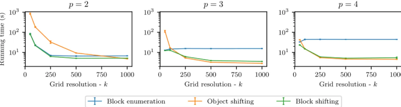
The computational effort required by sparse computation also depends on the number of dimensions pof the low-dimensional space. For example, the number of (adjacent) blocks, and the number of required shifts for object shifting and block shifting grow exponentially in p. To explore the impact of the dimension of the low-dimensional space on runtime, we applied the different algorithms to the COV dataset with p = 2, 3, and 4. As shown in Figure 2.7, the runtime of sparse computation with block enumeration increases steadily as p is increased even though the number of selected pairs decreases with increasing grid resolution. Sparse computation with object shifting and block shifting scales much better

(30)

0 250 500 750 1000 Grid resolution -k 101 102 103 Running time (s) p= 2 0 250 500 750 1000 Grid resolution -k 101 102 103 p= 3

Block enumeration Object shifting Block shifting

0 250 500 750 1000 Grid resolution -k 101 102 103 p= 4

Figure 2.7: Effect of the number of dimensions in the low-dimensional space, p, on the mean runtimes of sparse computation with block enumeration, object shifting, and block shifting for the COV dataset. The error bars indicate the standard deviation of the runtimes. Grid resolution is measured with respect to sparse computation with block enumeration.

with increasing values of p.

2.4 Compression for Massively-Large Datasets:

Sparse-Reduced Computation

Sparse-reduced computation is an extension of sparse computation. The idea of sparse computation is to avoid the computation of very small similarities as they are unlikely to affect the classification result. Sparse-reduced computation not only avoids the computation of very small similarities, but also avoids the computation of similarities between highly-similar and identical objects. Intuitively, sparse-reduced computation not only “rounds” very small similarities to zero but it also “rounds” very large similarities to one. Sparse-reduced computation consists of the four steps of data projection, space partitioning, data reduction, and similarity computation.

Data projection: The first step in sparse-reduced computation coincides with what is done in sparse computation. The d-dimensional dataset is projected onto a p-dimensional space, where pd. This is implemented using a sampling variant of principal component analysis called Approximate PCA [Hochbaum and Baumann, 2014]. Approximate PCA computes principal components that are very similar to those computed by exact PCA as shown in [Drineas et al., 2006], yet requires drastically reduced running time. Approximate PCA is based on a technique devised by [Drineas et al., 2006]. The idea is to compute exact PCA on a submatrixW of the original matrix A. The submatrix W is generated by random selection of columns and rows of A with probabilities proportional to the L2 norms of the

(31)

x

y z

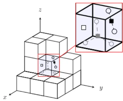
Figure 2.8: Data reduction with resolution k = 3 and κ = 1. As shown in the magnified block, the negative training objects (gray), the positive training objects (white fill), and the testing objects (black) are each replaced by a single representative.

Space partitioning: Once all objects are mapped into the p-dimensional space, the next step is to subdivide, in each dimension, the subspace occupied by the objects into k intervals of equal length. This partitions thep-dimensional space into kp _{grid blocks. Using a uniform}

value ofk for all dimensions allows us to control the total number of grid blocks with a single parameter. In the following, parameter k is referred to as the grid resolution. Each object is assigned to a single block based on the respective intervals in which itsp coordinates fall.

Data reduction: The grid is then used to reduce the size of the dataset by replacing so-called δ-identical objects by a single representative. Let δ = 1_κ for κ ∈ _N. In order to identifyδ-identical objects we subdivide each block into κp _{sub-blocks. The sub-blocks are}

obtained by partitioning the grid block along each dimension into κ intervals of equal length. For each sub-block, we replace objects of the same type (negative training objects, positive training objects and testing objects) by a single representative. For example, if κ= 1, then all objects of the same type that fall in the same grid block are considered δ-identical and are thus grouped together. If κ= 2 for a three-dimensional space, then the grid block is split into 23 _{= 8 sub-blocks and the replacement of objects by representatives is done for each}

sub-block separately. Different values for κ can be selected for different blocks to account for an unequal distribution of the data. The representatives are computed as the center of gravity of the corresponding objects and have a multiplicity weight equivalent to the number of objects they represent. Note that a representative may represent a single object. Figure 2.8 illustrates the data reduction step for a three-dimensional grid and κ= 1.

Similarity computation: The sparse similarity matrix on the representatives is computed based on the concept of grid neighborhoods. This concept is borrowed from image segmenta-tion where similarities are computed only between adjacent pixels [Hochbaum et al., 2013]. Here, we use the space partitioning and first consider all representatives in the same block to be adjacent and thus have their similarities computed. Then, adjacent blocks are identified and the similarities between representatives in those blocks are computed. Two blocks are

(32)

adjacent if they are within a one-interval distance from each other in each dimension (the

L∞ metric). Hence, for each block, there are up to 3p−1 adjacent blocks. The similarities

are computed in the original d-dimensional space. For very high-dimensional datasets, the similarities could also be computed in the low p-dimensional space. A finer grid resolution (higher value of k) generally leads to a lower density of the similarity matrix. Notice that for

k = 2 all representatives are neighbors of each other, and thus we get the complete similarity matrix. The set of representatives and the generated similarity matrix constitutes the input to the classification algorithms. The class labels that are assigned to representatives will be passed on to each of the objects that they represent.

2.5 Experimental Analysis of Sparse-Reduced

Computation

We apply both sparse computation and sparse-reduced computation with two similarity-based classifiers to five datasets. A comparison with existing sparsification approaches is not possible because these approaches require to first compute the full similarity matrix, which would exceed the memory capacity of our machine.

Similarity-based classifiers

We present two similarity-based machine learning techniques as binary classifiers that assign a set of testing objects to either the positive or the negative class based on a set of training objects. The two techniques are the K-nearest neighbor algorithm and the supervised normalized cut algorithm [Hochbaum, 2010].

K-nearest neighbor algorithm (KNN): The KNN algorithm [Fix and Hodges, 1951] finds the K nearest training objects to a testing object and then assigns the predominant class among those K neighbors. We use the euclidean metric to compute distances between objects and the nearest training object is used to break ties. When KNN is applied with sparse-reduced data, we consider the multiplicity weight of the representatives to determine the K nearest training representatives. For example, if K = 3 and the nearest training representative is positive and has a multiplicity weight of 2 and the second nearest training representative is negative and has a multiplicity weight of 5, the testing object is assigned to the positive class. A testing object is assigned to the negative class if all similarities to training objects are zero. In the experimental analysis we treatK as a tuning parameter.

Supervised normalized cut (SNC): SNC is a supervised version of HNC (Hochbaum’s Normalized Cut), which is a variant of normalized cut Hochbaum [2010]. We provide a detailed discussion of HNC in sectionsection 3.1, but we will give a short summary here for the purpose of these experiments.

(33)

HNC is defined on an undirected graph G= (V, E), where V denotes the set of nodes andE the set of edges. A weight wij is associated with each edge [i, j]∈E. A bi-partition of

a graph is called a cut, (S,S¯) ={[i, j] |i ∈ S, j ∈S¯}, where ¯S =V \S. Thecapacity of a cut (S,S¯) is the sum of weights of edges with one endpoint in S and the other in ¯S:

C(S,S¯) = X

i∈S,j∈_S,¯_[_i,j_]∈E wij.

In particular, the capacity of a set, S ⊂V, is the sum of edge weights within the setS,

C(S, S) = X

i,j∈S,[i,j]∈E wij.

In the context The nodes of the graph correspond to objects in the dataset and the edge weights wij quantify the similarity between the respective feature vectors associated with nodesi and j. Higher similarity is associated with higher weights.

The goal of one variant of HNC is to find a cluster that minimizes a linear combination of two criteria. One criterion is to maximize the total similarity of the objects within the cluster (the intra-similarity). The second criterion is to minimize the similarity between the cluster and its complement (the inter-similarity). A linear combination of the two criteria is minimized:

min

∅⊂S⊂V C(S,

¯

S)−λC(S, S). (2.1)

The relative weighting parameter λ is one of the tuning parameters.

The input graph for SHNC contains labeled nodes (training data) whose class label (either positive or negative) is known and unlabeled nodes. SNC is derived from HNC by assigning all labeled nodes with a positive label to the set S and all labeled nodes with a negative label to the set ¯S. The goal is then to assign the unlabeled nodes to either the setS or the set ¯S. For a given value of λ, this optimization problem is solved with a minimum cut procedure in polynomial time [Hochbaum, 2013b].

We implement SNC with Gaussian similarity weights. The Gaussian similarity between object i and j is defined as:

wij =e−α||xi−xj||2,

where parameter α represents a scaling factor, and xi and xj are the feature vector of

objects i and j. The Gaussian similarity function is commonly used in image segmentation, spectral clustering, and classification. When SNC is applied with sparse-reduced computation, we multiply each similarity value by the product of the weights of the two corresponding representatives. There are two tuning parameters: the relative weighting parameter of the two objectives, λ, and the scaling factor of the exponential weights, α. The minimum cut problems are solved with the MatLab implementation of the HPF pseudoflow algorithm version 3.23 of [Chandran and Hochbaum, 2009] that was presented in [Hochbaum, 2008].

(34)

Table 2.5: Datasets statistics (after modifications) Abbr # Objects # Features _{# Negatives}# Positives

COV 581,012 54 0.574 KDD 4,898,431 122 4.035 RLC 5,749,132 16 0.004 BOW2 8,499,752 234,151 0.037 RNG 10,000,000 20 1.000

datasets

We select four real-world datasets from the UCI Machine Learning Repository [Lichman, 2013] and one artificial datasets from previous studies [Breiman, 1996; Dong, Jian-xiong et al., 2005]. We substituted categorical features by a binary feature for each category. In the following, we briefly describe each dataset and mention further modifications that are made. The characteristics of the adjusted datasets are summarized in Table 2.5.

In the Bag of Words (BOW2) dataset, the objects are text documents from two different sources (New York Times articles and PubMed abstracts). A document is represented as a so-called bag of words, i.e. a set of vocabulary words. For each document, an vector indicates the number of occurrences of each word in the document. We treated New York Times articles as positives.

The dataset Covertype (COV) contains cartographic characteristics of forest cells in northern Colorado. There are seven different cover types which are labeled 1 to 7. Following [Caruana and Niculescu-Mizil, 2006], we treat type 1 as the positive class and types 2 to 7 as the negative class.

The dataset KDDCup99 (KDD) is the full dataset from the KDD Cup ’twork. Each

connection is labeled as either normal, or as an attack. We treat attacks as the positive class. In the dataset Record Linkage Comparison Patterns (RLC), the objects are comparison patterns of pairs of patient records. We substitute the missing values with value 0 and introduce an additional binary attribute to indicate missing values. The goal is to classify the comparison patterns as matches (the corresponding records refer to same patient) or non-matches. Matches are treated as positive class.

The dataset Ringnorm (RNG) is an artificial dataset that has been used in [Breiman, 1996] and [Dong, Jian-xiong et al., 2005]. The objects are points in a 20-dimensional space and belong to one of two classes. Following the procedure of [Dong, Jian-xiong et al., 2005], we generate a Ringnorm dataset instance with 10 million objects where each object is equally likely to be in either the positive or the negative class.

For each of the five datasets, we generate five subsets by randomly sampling 5,000, 10,000, 25,000, 50,000, and 100,000 objects from the full dataset.