Development of a Statistical Model for the Prediction of Overheating in UK Homes Using
Descriptive Time Series Analysis
Argyris Oraiopoulos
1, 2, Tom Kane
1, 2, Steven K Firth
1, 2, Kevin J Lomas
1, 21
Building Energy Research Group (BERG),
School of Civil and Building Engineering, Loughborough University, Loughborough, UK
2
London-Loughborough (LoLo) Centre for Doctoral Training on Energy Demand, Loughborough
University, Loughborough, UK
Abstract
Overheating risk in dwellings is often predicted using modelling techniques based on assumptions of heat gains, heat losses and heat storage. However, a simpler method is to use empirical data to predict internal temperatures in dwellings based on external climate data. The aim of this research is to use classical time series descriptive analysis and construct statistical models that allow the prediction of future internal temperatures based external weather data. Initial results from the analysis of a living room in a house show that the proposed method can successfully predict the risk of overheating based on four different overheating criteria.
Introduction
As global temperatures rise and the climate becomes more unstable, heatwaves will be a more common phenomenon The Health Protection Agency has stated that the number of heatwaves by 2020 will increase by 70% and over the next 70 years by 540% (HPA, 2012). A report by Vandentorren et al. (2004) estimated the excess deaths in France, during August 2003, at 14,800. In UK the number of excess deaths reached 2,139 and the increase to those over 75 years of age was 59% (Johnson et al., 2005). Stott et al. (2004) have estimated that a 2003-type summer is predicted to be average within Europe by 2040. This could cause in an increase of energy consumption in UK homes during summer periods due to a higher demand for cooling and hence an uptake in domestic air conditioning units, but it could also have a substantial impact on heat related morbidity and mortality rates and produce a series of challenges for the emergency services and the national health system (Grogan & Hopkins, 2002). According to Collins (2000), the effects of ambient temperature on physiological functions can be explained in terms of pathology. He marks, “fluctuations from an “ideal” range of hydrothermal conditions within dwellings and work places pose threat to health”. The risk of overheating in domestic buildings is frequently predicted using modelling methods based on assumptions of heat gains, heat losses and heat storage (Hacker et al., 2005, Porritt et al., 2012). The use of dynamic thermal simulation software requires the input of a number of assumptions that often lead to modelling errors and reduce confidence in the results. Recent large-scale data collection studies allow empirical approaches based on measurements alone. Such methods could base the prediction of
internal temperatures in dwellings, on previously recorded internal temperatures and external climate data. Time series analysis is such a method and it has been successfully used in fields such as economics, geophysics, control engineering and meteorology to describe, explain, predict and control processes (Chatfield, 1996). Time series data are not simply data collected over time; there has to exist some form of ordering. A definition is given by Bloomfield (1976), “A collection of numerical observations arranged in natural order with each observation associated with a particular instant of time or interval of the time which provides the ordering would qualify as time series data”.
The aim of the research presented in this paper is to present the methodology of applying the descriptive time series analysis and modelling in the field of building physics and more specifically to room temperature data. This novel approach is used to explore the mechanisms of the formation of such data series and to develop statistical models that allow the prediction of future temperatures based on past measured values and external climate data. The application of these statistical models, could lead to the provision of tailored advice to occupants on how and when to act in order to reduce indoor temperatures during hot summer conditions. It could also allow timely information to those caring for the elderly and infirmed in order to prevent adverse health impacts due to increased temperatures in enclosed spaces. By applying an empirical predictive model to national datasets, it can provide significant insights for the developments of future policies in mitigating overheating in homes across the country and allow for a more detailed plan to be issued in the event of a heatwave. Finally, with the aid of the latest developments in generating future external weather data for the 2030s, 2050s and 2080s (Eames et al., 2011), at-risk households can be supplied with information on how to reduce the risk of overheating in the future.
Methodology
DataThe data used in this study were collected in Leicester during the summer months of 2009 as part of the 4M project (Lomas et al., 2010), which focused on representing carbon emissions from different sources to measure the carbon footprint of the city of Leicester. Hobo pendant type temperature sensors were used to hourly record internal temperatures in the living rooms
and main bedrooms in 230 homes (411 internal spaces in total), from 1st July till the 31st August 2009. This data is a subset of a dataset that has already served as a solid basis for research projects focusing on indoor temperatures both in the summer (Lomas and Kane, 2013) and in winter (Kane et al., 2015). The external weather data were obtained from De Montfort University, located in the middle of Leicester, for the purposes of the 4M project, including the hourly measured external air temperature and solar irradiation. This paper is focusing on the analysis and modelling of a living room in one of the homes in the dataset.
Time series analysis
The steps in this analysis are based on the univariate time series modelling construction theory derived from the work of Box and Jenkins (1970). The first step in time series analysis is to do some initial analysis of the data, then to perform adjustments in order to identify the individual components of the series and subsequently estimate the components by modelling them and finally proceed with the forecasts. In identifying the individual components of an internal air temperature time series the following three components were considered.
Trend (T)
According to Chatfield (1996), the trend can be defined as “a long term change in the mean level” of a series.
Kendal & Ord (1990) explain that the trend represents the “smooth relatively slowly changing, features of the
time series over a considerable period of time”. For the
purposes of this work, the definition of trend has been taken as the one expressed by Kendal & Ord (1990) and the relative meaning of the phrase “a considerable period of time” defined as the length of the dataset, i.e.
62 days. Therefore, the long-term trend was considered as a form of the data that can represent the changes in the series from day to day over the 62-day monitoring period, i.e. the daily mean variation.
Seasonal Variation (S)
As Kendal & Ord (1990) describe, the definition of seasonality is by no means simple. They further note that seasonal effects have a degree of regularity but without defining a time period. Chatfield (1996) recommends that seasonal is a variation that is annual in period. For the purposes of this work, the definition of seasonal variation was based on Chatfield (1996) and since the extent of the data set was less than annual, the seasonal component was not be considered present in the series. Cyclical Component (C)
Similarly, to the seasonal variation, there is a debate in literature on what constitutes a cyclical variation. Kendal & Ord (1990) define seasonal variation as “cyclical itself” and give an example of a cyclical fluctuation as
the diurnal variations in temperature. Chatfield (1996) seems to agree with that example and further notes that “a cyclical change is one that exhibits variations at a fixed period due to some other physical cause”. For the purposes of this work the definition of cyclical variation
was based on the suggestions by Kendal & Ord (1990) and Chatfield (1996) that the diurnal fluctuations of internal temperatures do exhibit a cyclical pattern and can also be considered as the diurnal variation (the variation within a day). Once the individual components of the series were identified, the next step was the modelling of each one of them.
Results and discussion
This section presents the results for the individual models for the trend and the cyclical component as well as the evaluation of the complete model in terms of overheating prediction.
Internal air temperature trend analysis
Based on the aforementioned definition of the trend, the trend of the internal air temperature is given in the form of the daily mean of the hourly measured internal air temperature. For an hourly measured series θin,t,
t = {1, … , N, … , n}, the daily mean θ̅in,dis of the
following form:
θ̅in,d =
(θin,t=12am+ θin,t=1am+ ⋯ + θin,t=11pm)
24 (1)
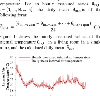
Figure 1 shows the hourly measured values of the internal temperature θin,t in a living room in a single home, and the calculated daily mean θ̅in,d .
Figure 1: Hourly measured internal air temperature ( 𝜃𝑖𝑛,𝑡 ) and daily mean ( 𝜃̅𝑖𝑛,𝑑 ) of one living room
The daily mean θ̅in,d represents the general trend (Tin,d)
of the internal air temperature, filtering out the daily swing of the internal air temperature around that daily mean. Having identified the general trend of the internal air temperature, the next step is to explore the trend of the external air temperature and develop a model that expresses the internal trend as a function of the external.
Tin,d= f(Tex,d) (2)
External air temperature trend analysis
This section explores the general trend of the external air temperature over the 62-day monitoring period. Since the living room under study is free-floating (no mechanical heating or cooling), the trend of the external air temperature will be the main driver of the general trend internal air temperature. A number of adjustments to the hourly external air temperature measured data to isolate the component of the trend have tested. Only the exponential weighted moving average (EWMA) of the
16 18 20 22 24 26 28 30 01/07/2009 01/08/2009 01/09/2009 In te rn a l A ir T em p er a tu re ( °C) Date
Hourly measured internal air temperature Daily mean internal air temperature
daily mean external air temperature was found to best correlate with the daily mean of the internal air temperature and consequently it was the one applied. Therefore, the trend of the external air temperature is given by the exponential weighted moving average of the external daily mean air temperature (θewma,ex,d),
which is of the following form:
θewma,t= (1 − α) ∑mn=0αnθt−n (3)
By expanding equation 3, following is derived:
θewma,ex,d= (1 − α) × (θex,d+ α θex,d−1+
α2 θ
ex,d−2+ α3 θex,d−3+ ⋯ + αm θex,d−m) (4)
Where θewma,ex,t is the exponentially weighted moving
average of the daily mean of the external air temperature; θex,d is the daily mean external air
temperature for today; θex,d−1 is the daily mean external
air temperature for the previous day; θex,d−2is the daily mean external air temperature for the day before and so on; αis a constant value between 0 and 1, according to which different weighting factors apply to θex,d−m and
m gives the amount of past days included in the model. Figures 2 and 3 show the effect that α and m have on
θewma,ex,d. Figure 2 shows the differences in θewma,ex,d
when using θex,d−m for m = 15 for all possible values
of α = {0 − 0.9}.
Figure 2:Exponentially weighted moving average of the external daily mean air temperature (θewma,ex,d ), using
the past 15 days (m=15) for all values of α between 0 and 0.9
From equation (4), it is clear that when α = 0, then
θewma,ex,d= θex,d and as the value of α increases, the
effect of the θewma,ex,d in reducing the diurnal variation
increases as well. In buildings, the correlation of the internal air temperature with θewma,ex,d using a high
value of α (α = 0.9) could indicate that the dwelling under study has higher thermal mass and therefore it responds to the external conditions at a slower rate (similar to the smoothed line for α = 0.9 in Figure 2) than a lightweight building where the internal air temperature conditions correlate better with a θewma,ex,d using lower value of α (α = 0.1 in Figure 2). It could
also indicate that the behaviour of the occupants is such that the internal air temperature is kept relatively constant regardless of the external conditions (i.e. keeping the blinds closed and the windows shut). It is important to note that when α = 0.9, the exponential nature of equation (4), means that it requires many more days than 15 to produce a meaningful value (one that is close to θex,d), therefore the use of this value should be
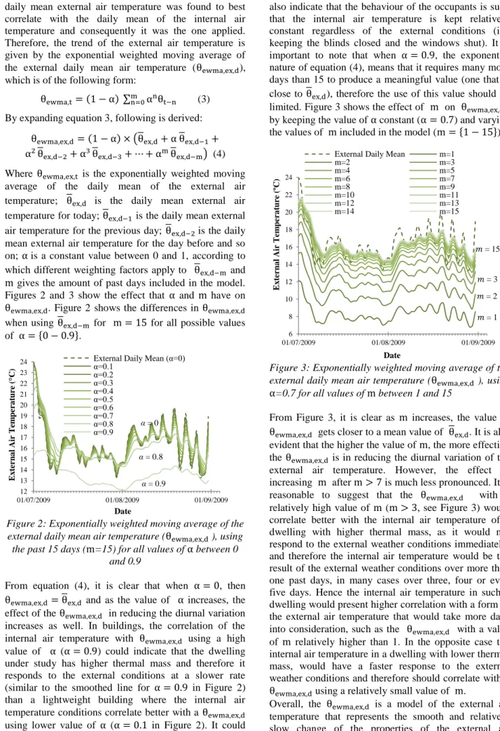
limited. Figure 3 shows the effect of m on θewma,ex,d ,
by keeping the value of α constant (α = 0.7) and varying the values of m included in the model (m = {1 − 15}).
Figure 3:Exponentially weighted moving average of the external daily mean air temperature (θewma,ex,d ), using
α=0.7 for all values of m between 1 and 15
From Figure 3, it is clear as m increases, the value of
θewma,ex,d gets closer to a mean value of θex,d. It is also
evident that the higher the value of m, the more effective the θewma,ex,d is in reducing the diurnal variation of the external air temperature. However, the effect of increasing m after m > 7 is much less pronounced. It is reasonable to suggest that the θewma,ex,d with a
relatively high value of m (m > 3, see Figure 3) would correlate better with the internal air temperature of a dwelling with higher thermal mass, as it would not respond to the external weather conditions immediately, and therefore the internal air temperature would be the result of the external weather conditions over more than one past days, in many cases over three, four or even five days. Hence the internal air temperature in such a dwelling would present higher correlation with a form of the external air temperature that would take more days into consideration, such as the θewma,ex,d with a value of m relatively higher than 1. In the opposite case the internal air temperature in a dwelling with lower thermal mass, would have a faster response to the external weather conditions and therefore should correlate with a
θewma,ex,d using a relatively small value of m.
Overall, the θewma,ex,d is a model of the external air temperature that represents the smooth and relatively slow change of the properties of the external air
12 13 14 15 16 17 18 19 20 21 22 23 24 01/07/2009 01/08/2009 01/09/2009 E x te rn a l A ir T em p er a tu re ( °C) Date
External Daily Mean (α=0) α=0.1 α=0.2 α=0.3 α=0.4 α=0.5 α=0.6 α=0.7 α=0.8 α=0.9 α = 0.9 α = 0.8 α = 0 6 8 10 12 14 16 18 20 22 24 01/07/2009 01/08/2009 01/09/2009 E x te rn a l A ir T em p er a tu re ( ºC ) Date
External Daily Mean m=1
m=2 m=3 m=4 m=5 m=6 m=7 m=8 m=9 m=10 m=11 m=12 m=13 m=14 m=15 𝑚 = 1 𝑚 = 2 𝑚 = 3 𝑚 = 15
temperature and therefore it can be considered a form of trend of the external air temperature, Tex,d . Therefore,
for this study the external air temperature trend is given by the following formula:
Tex,d= θewma,ex,d (5)
Internal air temperature trend modelling
This section presents the development of a model that is able to predict the trend of the internal air temperature in a living room, based on the trend of the external air temperature using simple linear regression analysis for a living room.
Since the living room is free-floating (meaning no mechanically assisted heating or cooling), it is expected that the changes in the internal air temperature are driven by the changes in the external temperature, thus the trend of the internal air temperature (Tin,d) can be a function of
the general trend of the external air temperature (Tex,d):
Tin,d= f(Tex,d)= f(a, m, θewma,ex,d) (6)
In expressing function (6), the parameters α and m of the θewma,ex,d can be optimised so that the correlation
between Tin,d and Tex,d is the highest possible. It is
essential therefore, to explore how many of the past days (m) need to be included in the equation and what is the optimum α value that gives the highest possible coefficient of determination (R2) between Tin,d and Tex,d.
In order to find which values of α and m are the highest R2 for the correlation between Tin,d and Tex,d , all m
values up to the past 15 days were tested. This was because it would be unlikely for the external weather conditions of 2 weeks past to have an effect on present internal air temperatures, and all values of α between 0.1 and 0.9. Figure 4 shows the results of the optimum R2 between Tin,d and Tex,d by using the optimum value of
α and including anything up to 15 past days in the
θewma,ex,d model.
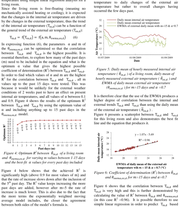
Figure 4: Optimum R2 between 𝜃̅𝑖𝑛,𝑑 of a living room and 𝜃𝑒𝑤𝑚𝑎,𝑒𝑥,𝑑 for varying m values between 1-15 days
and the best-fit 𝛼 values for every past day included
Figure 4 below shows that the achieved R2 is significantly high (above 0.9 for most values of m) and that the rate of increase slows down after the inclusion of the 5th past day. The R2 value keeps increasing the more past days are added, however after m=5 the rate of increase is much lower. This is also due to the fact that the more terms the exponentially weighted moving average model includes, the closer the agreement between both sides of the model’s formula is.
Consequently, it is concluded, that the daily mean of the internal air temperature can be expressed as a form of the external air temperature by using the exponentially weighted moving average (EWMA) of the daily mean external air temperature. Figure 5 shows that the daily mean internal air temperature follows a much more similar pattern to the exponentially weighted moving average of the daily mean external air temperature than just the daily mean of the external air temperature itself. This is due to the thermal mass of a dwelling that does not allow the immediate response of the internal air temperature to daily changes of the external air temperature but rather to overall changes having occurred the few days past.
Figure 5: Daily mean of hourly measured internal air temperature ( 𝜃̅𝑖𝑛,𝑑 ) of a living room, daily mean of
hourly measured external air temperature ( 𝜃̅𝑒𝑥,𝑑 ) and
EWMA of daily mean external air temperature (𝜃𝑒𝑤𝑚𝑎,𝑒𝑥,𝑑 ) for 𝑚=15 days and 𝛼 =0.7
It is therefore clear that the use of the EWMA produces a higher degree of correlation between the internal and external trends Tin,d and Tex,d than using the daily mean
of the external air temperature ( θex,d ) .
Figure 6 presents a scatterplot between Tin,d and Tex,d for this living room and also demonstrates the best fit line and the equation that produces it.
Figure 6: Coefficient of determination (R2) between 𝜃̅𝑖𝑛,𝑑
and 𝜃𝑒𝑤𝑚𝑎,𝑒𝑥,𝑑 for 𝑚=15 days and 𝛼=0.7
Figure 6 shows that the correlation between Tin,d and
Tex,d is very high and this is further demonstrated by
calculating the value of R2 between θ̅in,d and θewma,ex,d
(in this case R2 =0.96). It is possible therefore to use simple linear regression in order to predict Tin,d based
α= 0. 9 α= 0. 9 α= 0. 9 α= 0. 8 α= 0. 8 α= 0. 8 α= 0. 7 α= 0. 7 α= 0. 7 α= 0. 7 α= 0. 7 α= 0. 7 α= 0. 7 α= 0. 7 α= 0. 7 0.0 0.1 0.2 0.3 0.4 0.5 0.6 0.7 0.8 0.9 1.0 0 1 2 3 4 5 6 7 8 9 10 11 12 13 14 15 Op ti m u m R 2 Past days (m) 8 12 16 20 24 28 32 01/07/2009 01/08/2009 01/09/2009 A ir T em p er a tu re ( °C) Date
Daily mean internal air temperature Daily mean external air temperature
EWMA of external daily mean with m=15 & α=0.7
y = 1.07x - 5.69 R² = 0.96 12 16 20 24 28 18 20 22 24 26 28 D a il y m ea n i n te rn a l a ir te m p er a tu re ( °C)
EWMA of daily mean of the external air temperature wih 𝑚 = 15 & 𝛼 = 0.7 (°C)
on Tex,d . In that case the measured Tex,d will be the explanatory variable and the predicted T′in,d will be the
dependent variable and the equation will be of the following form:
T′
in,d= i + g × Tex,d (7)
Where T′in,d is the predicted (modelled) internal air
temperature trend and i and g are the intercept and the gradient of the best-fit line of the linear regression between the measured Tin,d and Tex,d . Figure 7 shows a
relatively high level of agreement between the measured internal trend (the daily mean internal air temperature) and the modelled internal trend (the resulted series from the linear regression between the daily mean internal air temperature and the exponentially weighted moving average of the daily mean external air temperature).
Figure 7: Measured internal trend (Tin,d) and modelled
internal trend (T′in,d)
Table 1 summarises the main measures of dispersion of the measured and the modelled trend as well as the residuals between them.
Table 1: Measures of dispersion for the measured and modelled trend and the hourly residuals between them
(ºC) Mean Max Min St. Dev.
Measured 20.8 25.5 18.7 1.4
Modelled 20.8 25.4 19.0 1.4
Residuals 0.00 0.68 -0.67 0.28
Table 1 shows that although the absolute maximum and minimum of the measured and modelled trend throughout the 62-day monitoring period are significantly close, the hourly residuals spread between -0.7°C and 0.7°C. The impact of this result however, should not be assessed before modelling the cyclical component of the internal air temperature and proceeding with the evaluation of the final model in terms of overheating prediction.
Internal air temperature cyclical component analysis This section explores the measured cyclical component of the internal air temperature over the 62-day monitoring period. This is calculated as the difference between the hourly measured internal air temperature and the daily mean of the internal air temperature.
However, as the scale of the hourly data is different from the daily mean, a transformation of the daily mean to a structured hourly series is essential. This is achieved by applying the daily mean as a single value, same for all hours throughout the 24-hour day. The cyclical component is then calculated by removing this hourly-applied daily mean series from the hourly values of the measured data. Figure 8 shows the hourly measured internal air temperature (θin,t) and the hourly-applied daily mean of the internal air temperature (θ̅in,t).
Figure 8: Hourly measured internal air temperature
(𝜽𝒊𝒏,𝒕) and hourly applied daily mean internal air temperature (𝜽̅𝒊𝒏,𝒕)
By removing the hourly-applied daily mean (θ̅in,t) from
the hourly measured series (θin,t), the cyclical
component of the internal air temperature (Cin,t) can be isolated and identified, hence:
Cin,t= θin,t− θ̅in,t (8)
This represents the diurnal variation around the mean of the internal air temperature and is given in Figure 9.
Figure 9: Cyclical component of the internal air temperature, (Cin,t)
Figure 9 shows the measured cyclical component (Cin,t)
of the internal air temperature of a living room during the 62-day monitoring period from 1st July 2009 till 31st August 2009. It can be seen that the cyclical component varies significantly during this period but the highest and some of the lowest values were recorded during the second half of August. Table 2 summarises the main measures of dispersion of the cyclical component of the internal air temperature (Cin,t) of this example living
room. 18 19 20 21 22 23 24 25 26 01/07/2009 01/08/2009 01/09/2009 In te rn a l A ir T em p er a tu re ( °C) Date
Measured Internal Trend Modelled Internal Trend
12 14 16 18 20 22 24 26 28 30 01/07/2009 01/08/2009 01/09/2009 In te rn a l A ir T em p er a tu re ( °C) Date
Hourly measured internal air temperature Daily mean internal air temperature (applied hourly) -3 -2 -1 0 1 2 3 01/07/2009 01/08/2009 01/09/2009 C y cl ic a l C o m p o n en t o f In te rn a l A ir T em p er a tu re ( °C) Date
Table 2: Measured of dispersion for the hourly values and the daily swing of the cyclical component of the internal air temperature of a living room
(ºC) Mean Max Min St. Dev.
Hourly 0.00 2.75 -1.27 0.60
Daily swing 1.84 4.02 0.67 0.79
Table 2 shows the range of values of the hourly measured cyclical component of the internal temperature (+2.75°C to -1.27°C) but it also shows that although overall the hourly mean is zero, the daily swing variation (daily maximum – daily minimum), has a mean value of 1.84°C and can range approximately between 0.7°C to 4°C.
As it has been the case with the component of the trend, the cyclical component will be expressed as a function of the external weather data, this time the external air temperature and the solar irradiation.
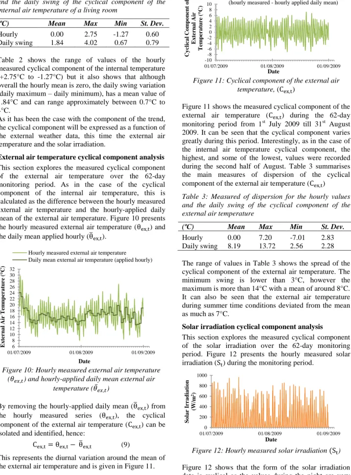
External air temperature cyclical component analysis This section explores the measured cyclical component of the external air temperature over the 62-day monitoring period. As in the case of the cyclical component of the internal air temperature, this is calculated as the difference between the hourly measured external air temperature and the hourly-applied daily mean of the external air temperature. Figure 10 presents the hourly measured external air temperature (θex,t) and the daily mean applied hourly (θ̅ex,t).
Figure 10: Hourly measured external air temperature (𝜃𝑒𝑥,𝑡) and hourly-applied daily mean external air
temperature (𝜃̅𝑒𝑥,𝑡)
By removing the hourly-applied daily mean (θ̅ex,t) from
the hourly measured series (θex,t), the cyclical
component of the external air temperature (Cex,t) can be
isolated and identified, hence:
Cex,t= θex,t− θ̅ex,t (9)
This represents the diurnal variation around the mean of the external air temperature and is given in Figure 11.
Figure 11: Cyclical component of the external air temperature, (Cex,t)
Figure 11 shows the measured cyclical component of the external air temperature (Cex,t) during the 62-day monitoring period from 1st July 2009 till 31st August 2009. It can be seen that the cyclical component varies greatly during this period. Interestingly, as in the case of the internal air temperature cyclical component, the highest, and some of the lowest, values were recorded during the second half of August. Table 3 summarises the main measures of dispersion of the cyclical component of the external air temperature (Cex,t)
Table 3: Measured of dispersion for the hourly values and the daily swing of the cyclical component of the external air temperature
(ºC) Mean Max Min St. Dev.
Hourly 0.00 7.20 -7.01 2.83
Daily swing 8.19 13.72 2.56 2.28
The range of values in Table 3 shows the spread of the cyclical component of the external air temperature. The minimum swing is lower than 3°C, however the maximum is more than 14°C with a mean of around 8°C. It can also be seen that the external air temperature during summer time conditions deviated from the mean as much as 7°C.
Solar irradiation cyclical component analysis
This section explores the measured cyclical component of the solar irradiation over the 62-day monitoring period. Figure 12 presents the hourly measured solar irradiation (St) during the monitoring period.
Figure 12: Hourly measured solar irradiation (St)
Figure 12 shows that the form of the solar irradiation data is cyclical as the values during the night are very close to zero and the daily peak occurs sometime during the day and that pattern is repeated every day, therefore
6 8 10 12 14 16 18 20 22 24 26 28 30 32 01/07/2009 01/08/2009 01/09/2009 E x te rn a l A ir T em n p er a tu re ( °C) Date
Hourly measured external air temperature
Daily mean external air temperature (applied hourly)
-10 -8 -6 -4 -2 0 2 4 6 8 10 01/07/2009 01/08/2009 01/09/2009 C y cl ic a l C o m p o n en t o f E x te rn a l A ir T em p er a tu re ( °C) Date
Cyclical Component of external air temperature (hourly measured - hourly applied daily mean)
0 200 400 600 800 1000 01/07/2009 01/08/2009 01/09/2009 S o la r Irr a d ia ti o n (W /m 2) Date
the cyclical component of the solar irradiation (Cs,t) will be considered as the hourly measured data. Consequently,
St= Cs,t (10)
It can also be observed that during the middle of the monitoring period (the second half of July and at the first half of August 2009), there are days when the solar irradiation drops to very low values. This could possibly have an effect on the risk of overheating in homes, reducing the heat stress in living rooms and bedrooms. Table 4 summarises the main measures of dispersion of the cyclical component of the solar irradiation (Cs,t).
Table 4: Measured of dispersion for the hourly values and the daily max of the cyclical component of the solar irradiation
(W/m2) Mean Max Min St. Dev.
Hourly 175.0 968.7 3.01 216.9
Daily Max 616.2 968.7 121.2 194.3
Table 4 shows that the spread of the maximum solar irradiation during a day is very large. The standard deviation of the daily maximum is almost as high as the one of the hourly values and this is a distinct feature of the climate in the UK, where during the summer, the hours of sunshine are limited due to high proportion of cloud cover.
Internal air temperature cyclical component modelling
This section presents the development of a model that is able to predict the cyclical component of the internal air temperature (Cin,t) in a living room, based on the cyclical
components of the external air temperature (Cex,t) and the solar irradiation (Cs,t), using a linear equation. Since
the example living room is free-floating (meaning no mechanically assisted heating or cooling), it is expected that the changes in the cyclical component of the internal air temperature are mainly driven by the changes in the cyclical components of the external temperature and the solar irradiation. Therefore, the cyclical component of the internal air temperature is a function of the cyclical components of the external temperature and the solar irradiation
Cin,t= f(Cex,t , Cs,t) (11)
The equation that is used to calculate the predicted cyclical component of the internal temperature (C′in,t)
comprises of five coefficients that are responsible for capturing the behaviour of the cyclical component of the internal temperature in relation to the cyclical components of the external air temperature and the solar irradiation
C′
in,t= A × Cex,φe+ B × Cs,φs+ γ (12)
Where A is the amplitude of the cyclical component of the external air temperature, φe is the phase of the cyclical component of the external air temperature, B is
the amplitude of the cyclical component of the solar irradiation, φs is the phase of the cyclical component of the solar irradiation and γ is a constant.
The coefficients A and B are responsible for capturing the extent of the effect of the external air temperature and solar irradiation respectively, on the cyclical component of the internal air temperature, in terms of the range of values of the model, as a result of factors such as the thermal mass of the dwelling, the orientation of the room, the use of blinds or other factors including the occupants’ actions. The phases φe and φs are
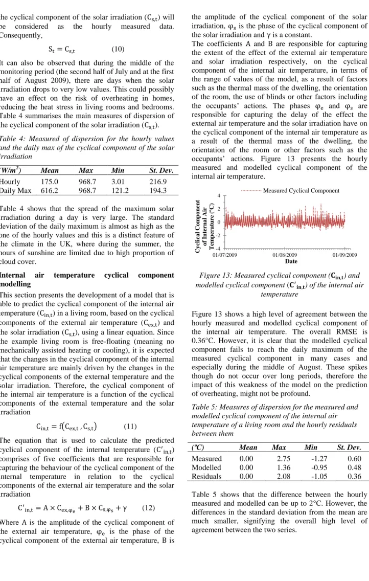
responsible for capturing the delay of the effect the external air temperature and the solar irradiation have on the cyclical component of the internal air temperature as a result of the thermal mass of the dwelling, the orientation of the room or other factors such as the occupants’ actions. Figure 13 presents the hourly measured and modelled cyclical component of the internal air temperature.
Figure 13: Measured cyclical component (𝐂𝐢𝐧,𝐭) and
modelled cyclical component (𝐂′𝐢𝐧,𝐭) of the internal air
temperature
Figure 13 shows a high level of agreement between the hourly measured and modelled cyclical component of the internal air temperature. The overall RMSE is 0.36°C. However, it is clear that the modelled cyclical component fails to reach the daily maximum of the measured cyclical component in many cases and especially during the middle of August. These spikes though do not occur over long periods, therefore the impact of this weakness of the model on the prediction of overheating, might not be profound.
Table 5: Measures of dispersion for the measured and modelled cyclical component of the internal air temperature of a living room and the hourly residuals between them
(ºC) Mean Max Min St. Dev.
Measured 0.00 2.75 -1.27 0.60
Modelled 0.00 1.36 -0.95 0.48
Residuals 0.00 2.08 -1.05 0.36
Table 5 shows that the difference between the hourly measured and modelled can be up to 2°C. However, the differences in the standard deviation from the mean are much smaller, signifying the overall high level of agreement between the two series.
-4 -2 0 2 4 01/07/2009 01/08/2009 01/09/2009 C y cl ic a l C o m p o n en t o f In te rn a l A ir T em p er a tu re ( ºC ) Date
The ITCC Model
The Internal Trend and Cyclical Component (ITCC) model is the result of joining the two individual models of the trend and the cyclical component together. Therefore, the modelled internal air temperature at time t (θ′in,t) is given by:
θ′
in,t= T′in,t+ C′in,t (13)
By substituting equations (7) and (12) in (13), the final model equation is given by:
θ′
in,t= i + g × [(1 − α) × (θex,d+ α θex,d−1+ ⋯ +
αm θ
ex,d−m)] + A × Cex,φe+ B × Cs,φs− γ (14)
Where:
θ′
in,t hourly modelled internal air temperature
i intercept of the best fit line for the correlation between the mean daily temperature of the internal air temperature and the exponentially weighted moving average of the daily mean of the external air temperature
g gradient of the best fit line for the correlation between the mean daily temperature of the internal air temperature and the exponentially weighted moving average of the daily mean of the external air temperature
α constant between 0.00 and 1.00
θex,d daily mean of the external air temperature of
current day
θex,d−1 daily mean of the external air temperature of
1 past day
m amount of past days used in the formula for the exponentially weighted moving average of the daily mean of the external air temperature
θex,d−m daily mean of the external air temperature of
m past days
A numerical coefficient of the cyclical
component of the external air temperature
Cex,φe cyclical component of the external air
temperature
φe phase of the cyclical component of the
external air temperature
B numerical coefficient of the cyclical
component of the solar irradiation
Cs,φs cyclical component of the solar irradiation φs phase of the cyclical component of the solar
irradiation
γ Constant
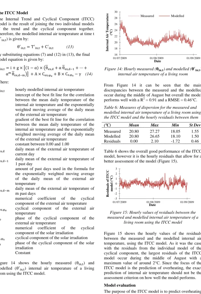
Figure 14 shows the hourly measured (θin,t) and modelled (θ′in,t) internal air temperature of a living
room using the ITCC model.
Figure 14: Hourly measured (𝛉𝐢𝐧,𝐭) and modelled (𝛉′𝐢𝐧,𝐭)
internal air temperature of a living room
From Figure 14 it can be seen that the main discrepancies between the measured and the modelled occur during the middle of August but overall the model performs well with a R2 = 0.91 and a RMSE = 0.46°C.
Table 6: Measures of dispersion for the measured and modelled internal air temperature of a living room using the ITCC model and the hourly residuals between them
(ºC) Mean Max Min St Dev
Measured 20.80 27.27 18.05 1.55
Modelled 20.80 26.65 18.10 1.50
Residuals 0.00 2.10 -1.72 0.46
Table 6 shows the overall good performance of the ITCC model, however it is the hourly residuals that allow for a better assessment of the model (Figure 15).
Figure 15: Hourly values of residuals between the measured and modelled internal air temperature of a
living room using the ITCC model
Figure 15 shows the hourly values of the residuals between the measured and the modelled internal air temperature, using the ITCC model. As it was the case with the residuals from the individual model of the cyclical component, the largest residuals of the ITCC model occur during the middle of August with a maximum value of around 2°C. Since the focus of the ITCC model is the prediction of overheating, the exact prediction of internal air temperature should not be the assessment criterion on how well the model performs. Model evaluation
The purpose of the ITCC model is to predict overheating and not the hourly internal air temperature, therefore the evaluation of the model will be based on four different overheating criteria. The static CIBSE criteria for living
16 18 20 22 24 26 28 30 01/07/2009 01/08/2009 01/09/2009 In te rn a l A ir T em p er a tu re (° C) Date Measured Modelled -3 -2 -1 0 1 2 3 01/07/2009 01/08/2009 01/09/2009 R esi d u a ls o f IT C C m o d el ( °C) Date
room temperatures suggest that the temperature should not exceed 25 °C for more than 5% of occupied hours per year and/or exceed 28 °C for more than 1% of occupied hours per year (CIBSE, 2006). In BSEN15251, the assessment of overheating is based on threshold comfort envelopes that increase at 0.33 K per K, as the running mean external temperature (Trm) increases from 10 °C to 30 °C, resulting in four categories of thermal comfort expectation (BSI, 2007). In the 2013 release of the TM52 document, CIBSE published their latest report on the limits of thermal comfort. The document outlines three criteria for free-running buildings (outlined below) and according to this assessment, if a room or a building fails to meet two out of the three, then it is classed as overheated (CIBSE, 2013). The American Society of Heating, Refrigerating and Air-Conditioning Engineering (ASHRAE) standard 55, operates in a similar was and the BSEN15251. The comfort envelopes however increase at a 0.31 K per K rate as the monthly mean external temperature (Tmm) increases from 10 °C to 33.5 °C (ANSI/ASHRAE, 2010).
The evaluation of the model therefore was based on comparing the results between the measured and the modelled internal air temperature in terms of overheating, using the aforementioned criteria as shown in Table 7.
Table 7: Assessment of measured and predicted overheating of a living room, using the ITCC mode according to four different overheating criterial
Criteria Measured Modelled
CIBSE Static % >25C 2.4 3.1 % >28C 0 0 Overheating No No CIBSE TM52 Criterion 1 (%) 0 0 Criterion 2 (K) 0 0 Criterion 3 (K) 0 0 Overheating No No BSEN15251 Category I (%) 0.2 0 Category II (%) 0 0 Category III (%) 0 0 Overheating No No ASHRAE 55 (%) 0.7 0.5 Overheating No No
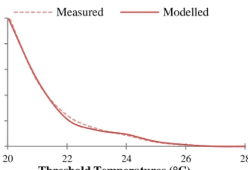
Table 7 shows that the ITCC model predicts the occurrence of overheating in this living room accurately using any of the main overheating criteria. However as this particular living room does not present severe overheating, another way of assessing its performance is to compare the number of hours during which the internal air temperature exceeds certain temperature thresholds, between the measured and the modelled internal air temperature. Figure 16 shows that the ITCC
model predicts accurately the number of hours above any temperature threshold.
Figure 16: Number of hours when the internal air temperature exceeds threshold temperature for the measured and the modelled internal air temperature
using the ITCC model for a living room.
Conclusion
The aim of this paper is to present the methodology of applying the descriptive time series analysis in order to develop an empirically derived parsimonious model that can be used to predict the risk of overheating in UK homes. The method is applied in a dwelling in Leicester, UK, using the internal air temperatures measured in the living room, between 1st July and 31st August 2009. This novel approach in analysing and modelling the internal air temperature in homes, requires the decomposition of the series in two individual components. The trend, responsible for capturing the long term change in the mean level, and the cyclical component, respondible for capturing the diurnal variation of the internal air temperature. Two different approaches are applied for modelling these two components and the final model is the result of joining these two. The Internal Trend and Cyclical Component (ITCC) model uses past values of internal air temperature together with past and future values of external air temperature and solar irradiation and is able to accurately predict overheating, based on four widely used overheating criteria. These criteria evaluate thermal comfort in terms of operative tempeature. However, thermal comfort is a function of both the operative tempeature and the humidity in internal spaces. Moreover, measuring the exact operative tempeature in occupied spaces is a rather difficult task (Lomas and Porritt, 2017).
The ITCC model was developed using only
measurements of internal air temperatures, external air temperatures and solar irradiation and no information regarding the houses or the occupants’ behaviour was used. The developement and validation of a dynamic thermal simulation model of a home that can produce predictions of overheating risk to a high level of accuracy could prove largely time consuming. The presented methodology however, suggests that it is possible to predict the risk of overheating indwellings, simply by measuring the interal air temperature and by using external weather data. Future publications will address the validation of the ITCC model using the
0 200 400 600 800 1000 20 22 24 26 28 N u m b er o f h o u rs w h en In te rn a l A ir T em p er a tu re ex ce ed s T h re sh o ld T em p er a tu re Threshold Temperatures (°C) Measured Modelled
current dataset (411 internal spaces) and other datasets (lightweight buildings, energy efficient homes, different climates) as well as the impact of the proximity (accuracy) of the weather data to the prediction of the overheating risk. The application of the ITCC model, could lead to the provision of tailored advice to occupants, and especially the elderly and those caring for them, on how and when to act in order to reduce indoor temperatures during hot summer conditions. In addition, by applying the ITCC model to national datasets, it can provide significant insights for the developments of future policies in mitigating overheating in homes across the country and allow for a more detailed plan to be issued in the event of a heatwave. Finally, with the aid of future external weather data for the 2030s, 2050s and 2080s, at-risk households can be supplied with information on how to reduce the risk of overheating in the future.
Acknowledgement
This research was made possible by the support from the Engineering and Physical Sciences Research Council (EPSRC) for the London-Loughborough Centre for Doctoral Research in Energy Demand (grant EP/H009612/1). The 4M consortium was funded by the EPSRC under their Sustainable Urban Environment programme (grant EP/F007604/1).
References
ANSI/ASHRAE, 2010. Standard 55-2010: Thermal environmental conditions for human occupancy. Atlanta, GA: Atlanta, GA : American Society of Heating, Refrigerating and Air-Conditioning Engineers.
Bloomfield, P. (1976) Fourier analysis of time series: an introduction. New York: John Wiley.
Box, G.E.P., Jenkin.s, G.M. (1970). Time series analysis: forecasting and control. San Francisco: Holden-Day.
BSI, 2007. BS EN 15251: 2007. Indoor environmental input parameters for design and assessment of energy performance of buildings addressing indoor air quality , thermal environment , lighting and acoustics. London: British Standards Institution. Chatfield, C. (1996). The analysis of time series: an
introduction.5th ed. London: Chapman & Hall. Collins, K., 2000. Cold, cold housing and respiratory
illnesses. In: Rudge, J., Nicol, F., eds. Cutting the cost of cold : affordable warmth for healthier homes. London: E & FN Spon.
CIBSE, 2006. Guide A. Environmental design. London: Chartered Institution of Building Services Engineers.
CIBSE, 2013. The limits of thermal comfort : avoiding overheating in European buildings. CIBSE TM52. pp. 1–25.
Eames, M., Kershaw, T., Coley, D. (2011). On the creation of future probabilistic design weather years from UKCP09. Building Services Engineering Research and Technology; 32, 127-42.
Grogan, H., Hopkins, P.M. (2002) Heat stroke: implications for critical care and anaesthesia. British Journal of Anaesthesia; 88, 700–07.
Johnson, H., Kovats, R., Mcgregor, G., Stedman, J., Gibbs, M., And Walton, H., 2005. The impact of the 2003 heat wave on daily mortality in England and Wales and the use of rapid weekly mortality estimates. In: lizabeth H. Gilles Brücker, Hélène Therre, ed. Euro surveillance. pp. 168–171.
Hacker, J.N., Belcher, S.E., Connell, R..K., (2005) Beating the Heat: keeping UK buildings cool in a warming climate. UKCIP Briefing Report. UKCIP. Oxford, UK.
Health Protection Agency (HPA) (2012). Health Effects of Climate Change in the UK 2012: current evidence, recommendations and research gaps. London, UK.
Kane, T., Firth S.K., Lomas, K.J., (2015). How are UK homes heated? A city-wide, socio-technical survey and implications for energy modelling. Energy and Buildings; 86, 817-832.
Kendal M., Ord, K., J. (1990) Time Series. 3rd Ed. London: Edward Arnold.
Lomas, K.J., Bell, M.C., Firth, S.K., Gaston, K.J., Goodman, P., Leake JR, Namdeo A, Rylatt M, Allinson D, Davies, Z.G., Edmondson, J.L., Galatioto, F., Brake, J.A., Guo, L., Fill, G., Irvine, K.N., Taylor, S.C., Tiwary, A. (2010). The carbon footprint of UK cities: 4M: measurement, modelling, mapping and management, ISOCARP Review 06, International Society of City and Regional Planners. p.168–91.
Lomas, K.J., Kane, T. (2013). Summertime temperatures and thermal comfort in UK homes. Building Research & Information; 41, 259-80.
Lomas, K.J. And Porritt, S.M., 2017. Overheating in buildings: lessons from research. Building Research & Information [online]. 45 (1–2), pp. 1–18.
Porritt, S.M., Cropper, P., Shao, L.C., Goodier, C.I. (2012). Ranking of interventions to reduce dwelling overheating during heat waves. Energy and Buildings; 55, 16-27.
Stott, P.A., Stone, D.A., And Allen, M.R., 2004. Human contribution to the European heatwave of 2003.
Nature. 432 (7017), pp. 610–614.
Vandentorren, S., Suzan, F., Medina, S., Pascal, M., Maulpoix, A., Cohen, J.C., And Ledrans, M., 2004. Mortality in 13 French cities during the August 2003 heat wave. American Journal of Public Health. 94 (9), pp. 1518–1520.