Deep Multi-State Dynamic Recurrent Neural
Networks Operating on Wavelet Based Neural
Features for Robust Brain Machine Interfaces
Benyamin Haghi1,*,Spencer Kellis2,Sahil Shah1,Maitreyi Ashok1,Luke Bashford2,Daniel
Kramer3,Brian Lee3,Charles Liu3,Richard A. Andersen2,Azita Emami1
1 Electrical Engineering Department, Caltech, Pasadena, CA, USA 2 Biology and Biological Engineering Department, Caltech, Pasadena, CA, USA 3 Neurorestoration Center and Neurosurgery, USC Keck School of Medicine, L.A., CA, USA
Abstract
We present a new deep multi-state Dynamic Recurrent Neural Network (DRNN) architecture for Brain Machine Interface (BMI) applications. Our DRNN is used to predict Cartesian representation of a computer cursor movement kinematics from open-loop neural data recorded from the posterior parietal cortex (PPC) of a human subject in a BMI system. We design the algorithm to achieve a reasonable trade-off between performance and robustness, and we constrain memory usage in favor of future hardware implementation. We feed the predictions of the network back to the input to improve prediction performance and robustness. We apply a scheduled sampling approach to the model in order to solve a statistical distribution mismatch between the ground truth and predictions. Additionally, we configure a small DRNN to operate with a short history of input, reducing the required buffering of input data and number of memory accesses. This configuration lowers the expected power consumption in a neural network accelerator. Operating on wavelet-based neural features, we show that the average performance of DRNN surpasses other state-of-the-art methods in the literature on both single- and multi-day data recorded over 43 days. Results show that multi-state DRNN has the potential to model the nonlinear relationships between the neural data and kinematics for robust BMIs.
1
Introduction
Brain-machine interfaces (BMIs) can help spinal cord injury (SCI) patients by decoding neural activity into useful control signals for guiding robotic limbs, computer cursors, or other assistive devices [1]. BMI in its most basic form maps neural signals into movement control signals and then closes the loop to enable direct neural control of movements. Such systems have shown promise in helping SCI patients. However, improving performance and robustness of these systems remains challenging. Even for simple movements, such as moving a computer cursor to a target on a computer screen, decoding performance can be highly variable over time. Furthermore, most BMI systems currently run on high-power computer systems. Clinical translation of these systems will require decoders that can adapt to changing neural conditions and which operate efficiently enough to run on mobile, even implantable, platforms.
Conventionally, linear decoders have been used to find the relationship between kinematics and neural signals of the motor cortex. For instance, Wu et al. [2] use a linear model to decode the neural activity of two macaque monkeys. Orsborn et al. [3] apply a Kalman filter, updating the model on batches of neural data of an adult monkey, to predict kinematics in a center-out task. Gilja et al. [4] propose
a Kalman Filter to predict hand movement velocities of a monkey in a center-out task. However, all of these algorithms can only predict piecewise linear relationships between the neural data and kinematics. Moreover, because of nonstationarity and low signal-to-noise ratio (SNR) in the neural data, linear decoders need to be regularly re-calibrated [2].
Recently, nonlinear machine learning algorithms have shown promise in attaining high performance and robustness in BMIs. For instance, Wessberg et al. [5] apply a fully-connected neural network to neural data recorded from a monkey. Shpigelman et al. [6] show that a Gaussian kernel outperforms a linear kernel in a Kernel Auto-Regressive Moving Average (KARMA) algorithm when decoding 3D kinematics from macaque neural activity. Sussillo et al. [7] apply a large FORCE Dynamic Recurrent Neural Network (F-DRNN) on neural data recorded from the primary motor cortex in two monkeys, and then they test the stability of the model over multiple days [8]. These nonlinear learning-based decoders are more stable and have improved performance compared to prior linear methods. However, they all have been applied on motor cortex data recorded from a non-human primate. Moreover, almost all of these decoders have been tested by using neural firing rates as input, which are not stable over long periods [2]. Recent work has demonstrated that neural activity in the posterior parietal cortex (PPC) can be used to support BMIs [9, 10, 11, 12], although the encoding of movement kinematics appears to be complex. Therefore, extracting appropriate neural features and designing a robust decoder that can model this relationship is required.
We propose a new Deep Multi-State Dynamic Recurrent Neural Network (DRNN) decoder to address the challenges of performance, robustness, and potential hardware implementation. We refer to two theorems to show the stability, convergence, and potential of DRNNs for approximation of state-space trajectories (see supplementary material). We train the DRNN by passing a history of input data to it and feeding the predictions of the system back to the input to improve performance and robustness for sequential data prediction. Moreover, we apply scheduled sampling to solve the statistical distribution discrepancy between the ground truth and predictions. By extracting different neural features, we compare the performance and robustness of the DRNN with the existing methods in the literature to predict hand movement kinematics from open-loop neural data. The data is recorded from the PPC of a human subject over 43 days. Finally, we discuss the potential for implementing our DRNN efficiently in hardware for implantable platforms. To the best of our knowledge, this is the first time that learning-based decoders have been used on human PPC activity. Our results indicate that the Deep Multi-State DRNN operating on mid-band wavelet-based neural features has the potential to model the nonlinear relationships between the neural data and kinematics for robust BMIs.
2
Deep multi-state dynamic recurrent neural network
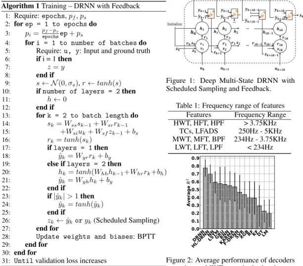
A DRNN is a nonlinear dynamic system described by a set of differential or difference equations. It contains both feed-forward and feedback synaptic connections. In addition to the recurrent ar-chitecture, a nonlinear and dynamic structure enables it to capture time-varying spatiotemporal relationships in the sequential data. Moreover, because of state feedback, a small recurrent network can be equivalent to a large feed-forward network. Therefore, a recurrent network will be compu-tationally efficient, especially for the applications that require hardware implementation [13]. We define our deep multi-state DRNN at each time stepkas below:
sk =Wsssk−1+Wsrrk−1+Wsiuk+Wsfzk+bs rk=tanh(sk) h(1)k =tanh(Wh(1)h(1)h (1) k−1+Wh(1)rrk+bh(1)) h(i)k =tanh(Wh(i)h(i)h (i) k−1+Wh(i)h(i−1)h (i−1) k +bh(i)) ˆ yk =Wyh(l)h (l) k +by ˆ yk =tanh(ˆyk), |yˆk|>1 zk←yˆkor yk (Scheduled sampling) (1)
s∈RN is the activation variable, andr∈RN is the vector of corresponding firing rates. These two
internal states track the first- and zero-order differential features of the system, respectively. Unlike conventional DRNNs,Wss∈RN×N generalizes the dynamic structure of our DRNN by letting the
network learn the matrix relationship between present and past values ofs.Wsr∈RN×N describes
the relationship betweensandr.Wsu∈RN×Irelatessto the input vectoru.zkmodels the added
lis the number of layers,Niis the number of hidden units inithlayer,h(i) ∈RNi is the hidden state of theith hidden layer,W
h(1)r ∈ RN1×N,Wh(i)h(i) ∈ RNi×Ni,Wh(i)h(i−1) ∈ RNi×Ni−1, Wyh(l) ∈ RM×Nl, bs ∈ RN,bh(i) ∈ RNi are the weights and biases of the network. All the hyper-parameters are learnable in our DRNN. Although feed-forward neural networks usually require a deep structure, DRNNs generally need fewer than three layers. Algorithm 1 shows the training procedure. Inference is performed by using equation 1. Figure 1 shows the schematic of our DRNN for a two layer network.
During inference, since the ground truth values are unavailable, the feedback,zk, has to be replaced
by the previous network predictions. However, the same approach cannot be applied during training since the DRNN has not been trained yet and it may cause poor performance of the DRNN. On the other hand, statistical discrepancies between ground truth and predictions mean that prior ground truth cannot be passed to the input. Because of this disparity between training and testing, the DRNN may enter unseen regions of the state-space, leading to mistakes at the beginning of the sequence prediction process. Therefore, we should find a strategy to start from the ground truth distribution and move toward the predictions’ distribution slowly as the DRNN learns.
There exist several approaches to address this issue. Beam search generates several target sequences from the ground truth distribution [14]. However, for continuous state-space models like recurrent networks, the effective number of generated sequences remains small. SEARN is a batch approach that trains a new model according to the current policy at each iteration. Then, it applies the new model on the test set to generate a new policy which is a combination of the previous policy and the actual system behavior [15]. In our implementation, we apply scheduled sampling which can be implemented easily in the online case and has shown better performance than others [16].
In scheduled sampling, at theithepoch of training, the model pseudorandomly decides whether to
feed ground truth (probabilitypi) or a sample from the predictions’ distribution (probability(1−pi))
back to the network, with probability distribution modeled byP(yk−1|rk−1). Whenpi = 1, the
algorithm selects the ground truth, and whenpi= 0, it works in Always-Sampling mode. Since the
model is not well trained at the beginning of the training process, we adjust these probabilities during training to allow the model to learn the predictions’ distribution. Among the various scheduling options forpi[16], we select linear decay, in whichpiis ramped down linearly frompstopf at each
epochepfor the total number of epochs,epochs: pi =
pf−ps
epochsep+ps (2)
3
Pre-processing and feature engineering
We evaluate the performance of our DRNN on 12 neural features: High-frequency, Mid-frequency, and Low-frequency Wavelet features (HWT, MWT, LWT); High-frequency, Mid-frequency, and Low-frequency Fourier powers (HFT, MFT, LFT); Latent Factor Analysis via Dynamical Systems (LFADS) features [17]; High-Pass and Low-Pass Filtered (HPF, LPF) data; Threshold Crossings (TCs); Multi-Unit Activity (MUA); and combined MWT and TCs (MWT + TCs) (Table 1). To extract wavelet features, we use ’db4’ mother wavelet on 50ms moving windows of the voltage time series recorded from each channel. Then, the mean of absolute-valued coefficients for each scale is calculated to generate 11 time series for each channel. HWT is formed from the wavelet scales 1 and 2 (effective frequency range≥3.75KHz). MWT is made from the wavelet scales 3 to 6 (234Hz -3.75KHz). Finally, LWT shows the activity of scales 7 to 11 as the low frequency scales (≤234Hz). Fourier-based features are extracted by computing the Fourier transform with the sampling frequency of 30KHz on one-second moving windows for each channel. Then, the band-powers at the same 11 scales of the wavelet features are divided by the total power at the frequency band of 0Hz - 15KHz. To generate TCs, we threshold bandpass-filtered (250Hz - 5KHz) neural data at -4 times the root-mean-square (RMS) of the noise in each channel. We do not sort the action potential waveforms [18]. Threshold crossing events were then binned at 50ms intervals.
LFADS is a generalization of variational auto-encoders that can be used to model time-varying aspect of neural signals. Pandarinath et al. [17] shows that decoding performance improved when using LFADS to infer smoothed and denoised firing rates. We used LFADS to generate features based on the trial-by-trial threshold crossings from each center-out task.
Algorithm 1Training – DRNN with Feedback 1: Require: epochs,pf,ps 2: forep = 1 to epochsdo 3: pi= pf−ps epochsep+ps
4: fori = 1 to number of batchesdo
5: Require:u, y: Input and ground truth
6: ifi = 1then
7: z=y
8: end if
9: s← N(0, σs),r←tanh(s)
10: ifnumber of layers = 2then
11: h←0
12: end if
13: fork = 2 to batch lengthdo 14: sk=Wsssk−1+Wsrrk−1
15: +Wsiuk+Wsfzk−1+bs
16: rk =tanh(sk)
17: iflayers = 1then
18: yˆk =Wyrrk+by
19: else iflayers = 2then
20: hk=tanh(Whhhk−1+Whrrk+bh) 21: yˆk =Wyhhk+by 22: end if 23: if|yˆk|>1then 24: yˆk =tanh(ˆyk) 25: end if 26: zk←yˆkoryk(Scheduled Sampling) 27: end for
28: Update weights and biases: BPTT
29: end for
30: end for
31: Untilvalidation loss increases
Figure 1: Deep Multi-State DRNN with Scheduled Sampling and Feedback.
Table 1: Frequency range of features
Features Frequency Range
HWT, HFT, HPF > 3.75KHz TCs, LFADS 250Hz - 5KHz MWT, MFT, BPF 234Hz - 3.75KHz LWT, LFT, LPF < 234Hz DRNN HL-DRNN NNLSTMGRURNN KARMAF-DRNNSVRXGBRFKFDTLM 0.0 0.1 0.2 0.3 0.4 0.5 0.6 0.7 0.8 0.9 Av er ag e R 2
Figure 2: Average performance of decoders operating on MWT over single-day data To extract HPF, MUA, and LPF features, we apply high-pass, band-pass, and low pass filters to the broadband data, respectively, by using second-order Chebyshev filters with cut-off frequencies of 234Hz and 3.75KHz. To infer MUA features, we calculate RMS of band-pass filter output. Then, we average the output signals to generate one feature per 50ms for each channel. Table 1 shows the frequency range of features.
We smooth all features with a 1s minjerk smoothing kernel. Afterwards, the kinematics and the features are centered and normalized by the mean and standard deviation of the training data. Then, to select the most informative features for regression, we use XGBoost, which provides a score that indicates how useful each feature is in the construction of its boosted decision trees [19, 20]. In our single-day analysis, we perform Principal Component Analysis (PCA). Figure 3 shows the block diagram of our BMI system.
Feature Extraction Smoothing Normalization Centering Feature Selection XGBoost PCA (Single-day Analysis) Center-Out Task Cursor Position
Figure 3: Architecture of our BMI system. Recorded neural activities of Anterior Intraparietal Sulcus (AIP), and Broadman’s Area 5 (BA5) are passed to a feature extractor. After pre-processing and feature selection, the data is passed to the decoder to predict the kinematics in a center-out task.
4
Experimental Results
We conduct our FDA- and IRB-approved study of a BMI with a 32 year-old tetraplegic (C5-C6) human research participant. This participant has Utah electrode arrays (NeuroPort, Blackrock Microsystems, Salt Lake City, UT, USA) implanted in the medial bank of Anterior Intraparietal Sulcus (AIP), and Broadman’s Area 5 (BA5). In a center-out task, a cursor moves, in two dimensions on a computer screen, from the center of a computer screen outward to one of eight target points located around a unit circle. During open-loop training, the participant observes the cursor move under computer control for 3 minutes. We collected open-loop training data from 66 blocks over 43 days for offline analysis of the DRNN. Broadband data were sampled at 30,000 samples/sec from the two implanted electrode arrays (96 channels each). Of the 43 total days, 42 contain 1 to 2 blocks of training data and 1 day contains 6 blocks, with about 50 trials per block. Moreover, these 43 days include 32, 5, 1, and 5 days of 2015, 2016, 2017, and 2018, respectively.
Since the predictions and the ground truth should be close in both micro and macro scales, we report root mean square error (RMSE) andR2as measures of average point-wise error and the strength
of the linear association between the predicted and the ground truth signals, respectively. Results reported in the body of the paper areR2values for Y-axis position.R2values for X-axis position and velocities in X and Y directions and RMSE values for all the kinematics are all presented in supplementary material. All the curves and bar plots are shown by using95%confidence intervals and standard deviations, respectively.
The available data is split into train and validation sets for parameter tuning. Parameters are computed on the training data and applied to the validation data. We perform 10 fold cross-validation by splitting the training data to 10 sets. Every time, the decoder is trained on 9 sets for different set of parameters and validated on the last set. We find the set of optimum parameters by using random search, as it has shown better performance than grid search [21]. Finally, we test the decoder with optimized parameters on the test set. The performance on all the test sets is averaged to report the overall performance of the models in both single- and multi-day analysis.
We compare our DRNN with other decoders, ranging from linear and historical decoders to nonlinear and modern techniques. The linear and historical decoders with which we compare ours are the Linear Model (LM) [2] and Kalman Filter (KF) [3]. The nonlinear and modern techniques with which we also compare ours include Support Vector Regression (SVR) [22], Gaussian KARMA [6], tree based algorithms (e.g., XGBoost (XGB) [19, 20], Random Forest (RF) [23], and Decision Tree (DT) [24]), and neural network based algorithms (e.g., Deep Neural Networks (NN) [5], Recurrent Neural networks with simple recurrent units (RNN) [25], Long-Short Term Memory units (LSTM) [26], Gated Recurrent Units (GRU) [27], and F-DRNN [7]). (See supplementary material).
We first present single-day performance of DRNN, which is a common practice in the field [7, 3, 28] and is applicable when the training data is limited to a single day. Moreover, there are aspects that differ between single- and multi-day decoding, which have not yet been well characterized (e.g., varying sources of signal instability) and remain challenging in neuroscience. Furthermore, single-day decoding is important before considering multi-day decoding since our implantable hardware will be developed such that the decoder parameters can be updated at any time.
4.1 Single-day performance
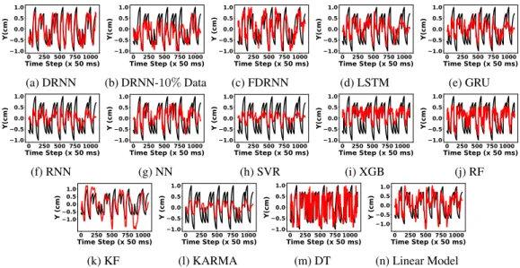
We select the MWT as the input neural feature. The models are trained on the first90%of a day and tested on the remaining10%. Figure 2 shows the average performance of the decoders. History-Less DRNN (HL-DRNN) uses the neural data at time k and kinematics at time k-1 to make predictions at time k. As we see, DRNN and HL-DRNN are more stable and have higher average performance. Figure 4 shows the regression of all the decoders on a sample day. We use only10%of the single-day training data in figure 4 (b) to show the stability of the DRNN to the limited amount of single-day training data. Other single-day analyses, including evaluation of the DRNN by changing the amount of single-day training data, the history of neural data, and the number of nodes are presented in supplementary material.
For cross-day analysis, we train the DRNN on a single day and test it on all the other days, and repeat this scenario for all the days. Figure 26 shows the performance of the DRNN over all the days. This figure shows that MWT is a more robust feature across single days.
0 250 500 750 1000 Time Step (x 50 ms) 1.0 0.5 0.0 0.5 1.0 Y(cm) (a) DRNN 0 250 500 750 1000 Time Step (x 50 ms) 1.0 0.5 0.0 0.5 1.0 Y(cm) (b) DRNN-10%Data 0 250 500 750 1000 Time Step (x 50 ms) 1.0 0.5 0.0 0.5 1.0 Y (cm) (c) FDRNN 0 250 500 750 1000 Time Step (x 50 ms) 1.0 0.5 0.0 0.5 1.0 Y(cm) (d) LSTM 0 250 500 750 1000 Time Step (x 50 ms) 1.0 0.5 0.0 0.5 1.0 Y(cm) (e) GRU 0 250 500 750 1000 Time Step (x 50 ms) 1.0 0.5 0.0 0.5 1.0 Y(cm) (f) RNN 0 250 500 750 1000 Time Step (x 50 ms) 1.0 0.5 0.0 0.5 1.0 Y (cm) (g) NN 0 250 500 750 1000 Time Step (x 50 ms) 1.0 0.5 0.0 0.5 1.0 Y (cm) (h) SVR 0 250 500 750 1000 Time Step (x 50 ms) 1.0 0.5 0.0 0.5 1.0 Y(cm) (i) XGB 0 250 500 750 1000 Time Step (x 50 ms) 1.0 0.5 0.0 0.5 1.0 Y(cm) (j) RF 0 250 500 750 1000 Time Step (x 50 ms) 1.0 0.5 0.0 0.5 1.0 Y (cm) (k) KF 0 250 500 750 1000 Time Step (x 50 ms) 1.0 0.5 0.0 0.5 1.0 Y (cm) (l) KARMA 0 250 500 750 1000 Time Step (x 50 ms) 1.0 0.5 0.0 0.5 1.0 Y(cm) (m) DT 0 250 500 750 1000 Time Step (x 50 ms) 1.0 0.5 0.0 0.5 1.0 Y (cm) (n) Linear Model
Figure 4: Regression of different algorithms on test data from the same day 2018-04-23: true target motion (black) and reconstruction (red).
0 5 10 15 20 25 30 35 40
Days
0.00
0.05
0.10
0.15
0.20
0.25
0.30
R 2 HWT MWT LWT HFT MFT LFT TCs LFADS LPF MUA HPF (a)MWT LPF LFADS LWT
TCs MUA MFT LFT HPF HFT HWT
0.0
0.1
0.2
0.3
Av
er
ag
e
R
2 (b)Figure 5: Cross-day analysis of the DRNN. 4.2 Multi-day performance
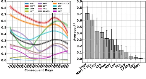
To evaluate the effect of the selected feature on the stability and performance of the DRNN, we train the DRNN on the data from the first 20 days of 2015 and test it on the consecutive days by using different features. Figure 6 shows that the DRNN operating on the MWT results in superior performance compared to the other features. Black vertical lines show the year change.
Then, we evaluate the stability and performance of all the decoders over time. Figure 30 shows that the overall and the average performance of the DRNN exceeds other decoders. Moreover, the DRNN shows almost stable performance across 3 years. The drop in the performance of almost all the decoders is because of the future neural signal variations [10].
To assess the sensitivity of the decoders to the number of training days, we change the number of training days from 1 to 20 by starting from day 20. Figure 8 shows that the Deep-DRNN with 2 layers and the DRNN have higher performance compared to the other decoders, even by using a small number of training days. Moreover, figure 8 shows that the performance of the DRNN with 1 layer, 10 nodes and history of 10 is comparable to the Deep-DRNN with 2 layers, 50 and 25 nodes in the first and second layers, and history of 20. Therefore, a small DRNN with a short history has superior performance compared to the other decoders.
21 22 23 24 25 26 27 28 29 30 31 32 33 34 35 36 37 38 39 40 41 42 43
Consequent Days
0.0
0.1
0.2
0.3
0.4
0.5
0.6
0.7
0.8
0.9
R
2 HWT MWT LWT HFT MFT LFT TCs LFADS MWT + TCs LPF MUA HPF (a)MWT
MWT + TCs
LWTLPFMUAMFTLFTTCsHPF
LFADSHFTHWT
0.0
0.1
0.2
0.3
0.4
0.5
0.6
0.7
0.8
0.9
Av
er
ag
e
R 2 (b)Figure 6: The DRNN operating on different features.
21 22 23 24 25 26 27 28 29 30 31 32 33 34 35 36 37 38 39 40 41 42 43
Consequent Days
0.0
0.1
0.2
0.3
0.4
0.5
0.6
0.7
0.8
0.9
R
2 Deep-DRNN DRNN HL-DRNN F-DRNN LSTM GRU RNN XGB RF DT SVR NN LM KF KARMA (a)DRNN
Deep-DRNN
KARMA
SVRXGB RF
HL-DRNN
NNLMRNNGRULSTMDT
F-DRNN
KF
0.0
0.1
0.2
0.3
0.4
0.5
0.6
0.7
Av
er
ag
e
R 2 (b)Figure 7: Multi-day performance of the decoders.
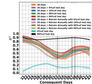
To evaluate the effect of re-training the DRNN, we consider four scenarios. First, we train DRNN on the first 20 days of 2015 and test it on the subsequent days. Second, we re-train a DRNN, which has been trained on 20 days, with the first5%,10%,50%, and90%of the subsequent test days. Third, we re-train the trained DRNN annually with5%,10%,50%, and90%of the first days of 2016, 2017, and 2018. Finally, we train DRNN only on the first5%and90%of the single test day. Figure 9 shows a general increase in the performance of the DRNN after the network is re-trained. The differences between the performances of the first three scenarios are small, which means that the DRNN does not necessarily need to be re-trained to perform well over multiple days. However, because of instability of the recorded neural data [10], training the DRNN on the first90%of the test day in the last scenario results in the highest average performance on the test day.
5
Hardware implementation potential
We are proposing a method that will not only have good performance on single- and multi-day data, but will also be optimal for hardware implementation. Since it is impractical to require powerful CPUs and GPUs for everyday usage of a BMI device, we need a device that is easily portable and does not require communication of the complete signals recorded by electrodes to an external computer for computation. Doing the computation in an Application Specific Integrated Circuit (ASIC) would
1 2 3 4 5 6 7 8 9 10 11 12 13 14 15 16 17 18 19 20
Number of Training Days
0.0
0.1
0.2
0.3
0.4
0.5
0.6
0.7
R
2 Deep-DRNN DRNN HL-DRNN F-DRNN LSTM GRU RNN XGB RF DT SVR NN LM KF KARMAFigure 8: Effect of number of training days on the performance of the decoders.
21 22 23 24 25 26 27 28 29 30 31 32 33 34 35 36 37 38 39 40 41 42 43 Consequent Days 0.0 0.1 0.2 0.3 0.4 0.5 0.6 0.7 0.8 0.9 1.0 R 2 20 days
20 days + 5% of test day 20 days + 10% of test day 20 days + 50% of test day 20 days + 90% of test day
20 days + Retrain Annually with 5% of test day 20 days + Retrain Annually with 10% of test day 20 days + Retrain Annually with 50% of test day 20 days + Retrain Annually with 90% of test day 5% of test day
90% of test day
Figure 9: The DRNN operating in different train-ing scenarios.
drastically reduce the latency of kinematics inference and eliminate a large power draw for the gigabytes of neural data that must be transferred otherwise. Thus, we plan to create an ASIC that can be implanted in the brain to perform inference of kinematics from neural signals. The main bottleneck in most neural network accelerators is the resources spent on fetching input history and weights from memory to the Multiplication and Accumulation (MAC) unit [29]. The DRNN will help mitigate this issue since we require fewer nodes and input history compared to the standard recurrent neural networks. This eliminates the need for large input history storage and retrieval, reducing latency and control logic. Furthermore, by using 16-bit fixed point values for the weights and inputs rather than floating point values, we can reduce the power used by the off-chip memory [29, 30].
6
Discussion
We propose a Deep Multi-State DRNN with scheduled sampling to better model the nonlinearity between the neural data and kinematics in BMI applications. We show that the added internal derivative state enables our DRNN to track first order and more complicated patterns in the data. Moreover, unlike conventional DRNNs, our DRNN learns a matrix that establishes a relationship between the past and present derivative states. To the best of our knowledge, this is the first demonstration of applying feedback and scheduled sampling to a DRNN to predict kinematics by using open-loop neural data recorded from the PPC area of a human subject. Our DRNN has the potential to be applied to the recorded data from other brain areas as a recurrent network.
To evaluate our DRNN, we analyze single-day, cross-day, and multi-day behavior of the DRNN by extracting 12 different features. Moreover, we compare the performance and robustness of the DRNN with other linear and nonlinear decoders over 43 days. Results indicate that our proposed DRNN, as a nonlinear dynamical model operating on the MWT, is a powerful candidate for a robust BMI. The focus of this work is to first evaluate different decoders by using open-loop data since the data presented was recorded from a subject who has completed participation in the clinical trial and has had the electrodes explanted. However, the principles learned from this analysis will be relevant to the future subjects with electrodes in the same cortical area.
Future studies will evaluate the DRNN performance in a closed-loop BMI, in which all the decoders use the brain’s feedback. Next, since we believe that our small DRNN achieves higher efficiency and uses less memory by reducing the history of the input, number of weights, and therefore memory accesses, we are planning to implement the DRNN in a field-programmable gate array (FPGA) system where we can optimize for speed, area, and power usage. Then, we will build an ASIC of the DRNN for BMI applications. The system implemented must be optimized for real-time processing. The hardware will involve designing multiply-accumulates with localized memory to reduce the power consumption associated with memory fetch and memory store.
Acknowledgment: We thank Tianqiao and Chrissy (T&C) Chen Institute for Neuroscience at California Institute of Technology (Caltech) for supporting this IRB approved research.
References
[1] Sam Musallam, BD Corneil, Bradley Greger, Hans Scherberger, and Richard A. Andersen. Cognitive control signals for neural prosthetics. Science, 305(5681):258–262, 2004.
[2] Wei Wu and Nicholas G. Hatsopoulos. Real-time decoding of nonstationary neural activity in motor cortex. IEEE Transaction on Neural Systems and Rehabilitation Engineering, 16(3):213– 222, 2008.
[3] Amy L. Orsborn, Siddharth Dangi, Helene G. Moorman, and Jose M. Carmena. Closed-loop decoder adaptation on intermediate time-scales facilitates rapid bmi performance improvements independent of decoder initialization conditions. IEEE Transactions on Neural Systems and Rehabilitation Engineering, 20(4):468–477, 2012.
[4] Vikash Gilja, Paul Nuyujukian, Cindy A. Chestek, John P. Cunningham, Byron M. Yu, Joline M. Fan, Mark M. Churchland, Matthew T. Kaufman, Jonathan C. Kao, Stephen I. Ryu, and Krishna V. Shenoy. A high-performance neural prosthesis enabled by control algorithm design.
Nature Neuroscience, 15(12):1752–1757, 2012.
[5] Johan Wessberg, Christopher R. Stambaugh, Jerald D. Kralik, Pamela D. Beck, Mark Laubach, John K. Chapin, Jung Kim, S. James Biggs, Mandayam A. Srinivasan, and Miguel A. L. Nicolelis. Real-time prediction of hand trajectory by ensembles of cortical neurons in primates.
Nature, 408:361–365, 2000.
[6] Lavi Shpigelman, Hagai Lalazar, and Eilon Vaadia. Kernel-arma for hand tracking and
brain-machine interfacing during 3d motor control. Advances in Neural Information Processing
Systems, 21, 2009.
[7] David Sussillo, Paul Nuyujukian, Joline M. Fan, Jonathan C. Kao, Sergey D. Stavisky, Stephen Ryu, and Krishna Shenoy. A recurrent neural network for closed-loop intracorti-cal brain–machine interface decoders. Journal of Neural Engineering, 9(2), 2012.
[8] David Sussillo, Sergey D. Stavisky, Jonathan C. Kao, Stephen I. Ryu, and Krishna V. Shenoy. Making brain–machine interfaces robust to future neural variability. Nature communications, 7(13749), 2016.
[9] Richard A. Anderson, Spencer Kellis, Christian Klaes, and Tyson Aflalo. Toward more versatile and intuitive cortical brain machine interfaces. Current Biology, 24(18):R885–R897, 2014.
[10] Tyson Aflalo, Spencer Kellis, Christian Klaes, Brian Lee, Ying Shi, Kelsie Pejsa, Kathleen Shanfield, Stephanie Hayes-Jackson, Mindy Aisen, Christi Heck, Charles Liu, and Richard A. Anderson. Decoding motor imagery from the posterior parietal cortex of a tetraplegic human.
Science, 348(6237):906–910, 2015.
[11] Christian Klaes, Spencer Kellis, Tyson Aflalo, Brian Lee, Kelsie Pejsa, Kathleen Shanfield, Stephanie Hayes-Jackson, Mindy Aisen, Christi Heck, Charles Liu, and Richard A. Andersen. Hand shape representations in the human posterior parietal cortex. Journal of Neuroscience, 35(46):15466–15476, 2015.
[12] Carey Y. Zhang, Tyson Aflalo, Boris Revechkis, Emily R. Rosario, Debra Ouellette, Nader Pouratian, and Richard A. Andersen. Partially mixed selectivity in human posterior parietal association cortex. Neuron, 95(3):697–708, 2017.
[13] Liang Jin, P.N. Nikiforuk, and M.M. Gupta. Approximation of discrete-time state-space trajectories using dynamic recurrent neural networks.IEEE transaction on automatic control, 40(7):1266–‘1270, 1995.
[14] Peng S. Ow and Thomas E. Morton. Filtered beam search in scheduling.International Journal for Production Research, 26(1):35–62, 1988.
[15] Hal Daume, John Langford, and Daniel Marcu. Search-based structured prediction.Machine Learning Journal, 2009.
[16] Samy Bengio, Oriol Vinayls, Navdeep Jaitly, and Noam Shazeer. Scheduled sampling for sequence prediction with recurrent neural networks. Neural Information Processing Systems (NIPS), 2015.
[17] Chethan Pandarinath, Daniel J. O’Shea, Jasmine Collins, Rafal Jozefowicz, Sergey D. Stavisky, Jonathan C. Kao, Eric M. Trautmann, Matthew T. Kaufman, Stephen I. Ryu, Leigh R. Hochberg, Jaimie M. Henderson, Krishna V. Shenoy, L. F. Abbott, and David Sussillo. Inferring single-trial
neural population dynamics using sequential auto-encoders.Nature Methods, 15:805—-815,
2018.
[18] Christie BP, Tat DM, Irwin ZT, Gilja V, Nuyujukian P, Foster JD, Ryu SI, Shenoy KV, Thompson DE, and Chestek CA. Comparison of spike sorting and thresholding of voltage waveforms for intracortical brain-machine interface performance.Journal of Neural Engineering, 12(1):1741— -2560, 2015.
[19] Tianqi Chen and Carlos Guestrin. Xgboost: A scalable tree boosting system.arXiv, 2016.
[20] Mahsa Shoaran, Benyamin A. Haghi, Milad Taghavi, Masoud Farivar, and Azita Emami. Energy-efficient classification for resource-constrained biomedical applications.IEEE Journal on Emerging and Selected Topics in Circuits and Systems, 8(4):693—-707, 2018.
[21] James Bergstra and Yoshua Bengio. Random search for hyper-parameter optimization. Journal of Machine Learning Research, 13:281–305, 2012.
[22] Debasish Basak, Srimanta Pal, and Dipak Chandra Patranabis. Support vector regression.
Neural Information Processing, 11(10):203–224, 2007.
[23] Leo Breiman. Random forests.Journal of Machine Learning, 45(1):5—-32, 2001.
[24] J Ross Quinlan. Induction of decision trees. Journal of Machine Learning, 1(1):81—-106,
1986.
[25] Danilo P. Mandic and Jonathan A. Chambers. Recurrent Neural Networks for Prediction:
Learning Algorithms, Architectures and Stability. John Wiley & Sons, Inc., New York, NY, USA, 2001.
[26] Felix A. Gers, Jurgen Schmidhuber, and Fred Cummins. Learning to forget: Continual prediction with lstm.Neural Computation, 12(10):2451–2471, 2000.
[27] Kyunghyun Cho, Bart van Merrienboer, Caglar Gulcehre, Dzmitry Bahdanau, Fethi Bougares, Holger Schwenk, and Yoshua Bengio. Learning phrase representations using rnn encoder-decoder for statistical machine translation.arXiv, 2014.
[28] Suraj Gowda, Amy L. Orsborn, Simon A. Overduin, Helene G. Moorman, and Jose M. Carmena. Designing dynamical properties of brain-machine interfaces to optimize task-specific perfor-mance.IEEE Transactions on Neural Systems and Rehabilitation Engineering, 22(5):911—-920, 2014.
[29] Paul N. Whatmough, Sae Kyu Lee, David Brooks, and Gu-Yeon Wei. Dnn engine: A 28-nm timing-error tolerant sparse deep neural network processor for iot applications.IEEE Journal of Solid-State Circuits, 53(9):2722—-920, 2018.
[30] Mohit Shah, Sairam Arunachalam, Jingcheng Wang, David Blaauw, Dennis Sylvester, Hun Seok Kim, Jae sun Seo, and Chaitali Chakrabarti. A fixed-point neural network architecture for speech applications on resource constrained hardware. Journal of Signal Processing Systems, 90(9):725—-741, 2018.
[31] Lianfang Tian and Curtis Collins. A dynamic recurrent neural network-based controller for a rigid-flexible manipulator system. Mechatronics, 14(5):471–490, 2004.
[33] Fabian Pedregosa, Gael Varoquaux, Alexandre Gramfort, Vincent Michel, Bertrand Thirion, Olivier Grisel, Mathieu Blondel, Peter Prettenhofer, Ron Weiss, Vincent Dubourg, Jake Vander-plas, Alexandre Passos, David Cournapeau, Matthieu Brucher, Matthieu Perrot, and Edouard Duchesnay. Scikit-learn: Machine learning in python. Journal of Machine Learning Research, 12:2825–2830, 2012.
[34] Adam Paszke, Sam Gross, Soumith Chintala, Gregory Chanan, Edward Yang, Zachary DeVito, Zeming Lin, Alban Desmaison, Luca Antiga, and Adam Lerer. Automatic differentiation in pytorch. Neural Info Processing Systems, 31, 2017.
[35] Simon O. Haykin. Adaptive Filter Theory. Prentice Hall, Englewood Cliffs, NJ, USA, 2001.
A
Dynamic recurrent neural network
A general structure of a discrete-time DRNN is given by the following expressions:
sk=−ask−1+f(Wss, sk−1, Wsu, uk, bs)
ˆ
yk =Wyssk+by
(3)
wheres∈RN,yˆ∈RM, andu∈RI are the state, prediction, and the input vectors, respectively,
Wss∈RN×N,Wsu∈RN×I, andWys∈RM×N are the weight matrices,a∈[−1,1]is a constant
controlling state decaying,bs ∈RN, andby ∈RM are the biases, andf : RN ×RI →RN is a
vector-valued function. [13]
B
Approximation of state-space trajectories
Theorem 2.1 verifies the approximation capability of DRNNs for the discrete-time, and non-linear systems.
Theorem B.1 LetS ⊂RM andU ⊂RI be open sets,Ds⊂SandDu⊂Ube compact sets, and
f :S×U →RM be a continuous vector-valued function which defines the following non-linear system
zk=f(zk−1, uk), z∈RM, u∈RI (4) with an initial valuez0∈Ds. Then for an arbitrary number >0, and an integer0< L <∞, there exist an integer N and a DRNN of the form(1)with an appropriate initial states0such that for any bounded inputu:R+ = [0,+∞)→D
u
max
0≤k≤L||zk−sk||< (5)
Proof: See [13]
C
Local stability and convergence of DRNNs
Learning rate (γ) plays the main role in stability and convergence of neural networks. By using Lyapunov theorem, we define the range of the learning rate to guarantee the real-time convergence of DRNNs and the stability of the system during the whole control process.
Theorem C.1 If an input series of internal dynamic neural network can be activated in the whole control process subject touk∈RI, then learning rate satisfies
0< γ < 2
r2 (6)
wherer=∂W∂e,e= ˆy−yis the difference of prediction and ground-truth, and W is the concatenation of connection weights of each network unit. Then (4) ensures the system is exponentially convergent.
Proof: See [31]
D
Description of the other methods
Since all of these methods are well-known in the literature, we only provide a brief explanation of each here. We explain the F-DRNN with details since our network is a generalization of the F-DRNN, with all the parameters to be learnable. For more information, please take a look at the main references. We use Pytorch, Keras, Scikit-learn and Python 2.7 for simulations. [32, 33, 34]. D.1 Latent Factor Analysis via Dynamical Systems (LFADS) [17]
Latent Factor Analysis via Dynamical Systems (LFADS) works by modeling a dynamical system that can generate neural data. The algorithm models the nonlinear vector valued function F that
can infer firing rates using neural data input. The LFADS system is a generalization of variational auto-encoders that can be used with sequences of data, to model the time-varying aspect of neural signals. We use observed spikes as the input to the encoder RNN. We bin our spikes in 50 ms bins and then separate each center-out task into a separate trial. We use the inferred firing rates that are the result of applying a nonlinearity and affine transformation on the factors output from the generator RNN. A dimensionality of 64 was chosen for the latent variables that are the controller outputs and the factors.
D.2 FORCE Dynamic Recurrent Neural Network (F-DRNN) [7] F-DRNN is defined as below: τdst dt =−st−1+gWsrrt−1+βWsiut+Wsfyˆt−1+bs rt=tanh(st) ˆ yt=Wyrrt+by (7)
s∈ RN is the activation variable, andr∈RN is the vector of corresponding firing rates. These
states track the first and zero order differential features of the system, respectively.
Wsr ∈RN×N describes the relationship betweensandr.Wsu∈RN×Irelatessto the input vector
u.yˆmodels the feedback in the network.Wsf ∈RN×M tracks the effect ofyˆons.Wyr∈RM×N
indicates the linear transformation between the firing ratesrand the predictionyˆ.τ,g, andβare the neuronal time constant, scaling of internal connections, and scaling of inputs, respectively.
To discretize the first equation of the continuous F-DRNN, we integrate the first expression of the system by using the Euler method at a time step of∆t. Then, the equations of the network become:
sk = (1−c)sk−1+cgWsrrk−1+cβWsiuk+cWsfyˆk−1+cbs rk=tanh(sk) ˆ yk =Wyrrk+by (8) wherec= ∆tτ
In F-DRNN, we selectWsr,Wsi, andWsf to be randomly sparse, i.e., onlyn= 0.1N,i= 0.1I,
andm= 0.5M randomly chosen elements are zero in each of their rows, respectively. The non-zero elements of the matrices are drawn independently from non-zero-mean Gaussian distributions with variancesn1,1i, andm1, respectively.s0and the constant biasbsare drawn from zero-mean Gaussian
distributions with the standard deviationsσsandσb, respectively. Elements ofWyrare initialized
to zero. Since the only matrix learned in the network is the output weightWyrand all the other
weights are fixed, we name this network as FORCE DRNN [7]. Therefore, the network dynamics are controlled by the matrixgWsr+WsfWyr. To updateWyr, we use recursive least-squares (RLS)
algorithm [35]. The error signal is defined by:
ek = ˆyk−yk (9)
By definingPas the inverse correlation matrix, the equation for updatingPis as below: Pk =Pk−∆k−
Pk−∆krkrTkPk−∆k
1 +rT
kPk−∆krk
, P0=γI (10)
Whereγand∆kindicate learning rate and learning step size (batch size), respectively. The modifica-tion to themthcolumn ofW
yrby using themthelement of the error is:
Wyr(m) k
=Wyr(m)k−∆k−e (m)
k Pkrk (11)
D.3 Deep Neural Network [5]
In a fully connected neural network, there are multiple layers: an input layer, output layer, and any number of hidden layers with multiple nodes in each hidden layer. The output of each node in each layer is connected to the input of each node in the consecutive layer. Each node performs of
PN
i=1Wixi, wherexiis each input from the nodes in the previous layer andWiis the weight of the
to a normalized range using a function such astanhto get values between -1 and 1.Wiis trained
through a process called back-propagation that trains the network on the inputs and finds the error, iteratively minimizing the loss function until the error stays relatively constant.
Since over-fitting is possible, which can cause issues where the trained model cannot later generalize to the separate test data, we can try to perform early stopping during validation such that a limited number of epochs (round of training with all inputs) are used for training before the weights are finalized. The following number of epochs are considered in our work: 5, 10, 20, 30, 50, 75, 100, 125, 150, 200, 300, 400, 500, 600. In addition, we consider different network structures with up to 3 layers, where each set consists of 1, 2, or 3 hidden layers with the given number of nodes in each layer: (100), (100, 100), (100, 10), (20, 20), (20, 20, 20), (40, 40), (40, 10), (40, 40, 40), (10, 10, 10). D.4 Support Vector Regression [22]
Support vector regression (SVR) is the continuous form of support vector machines where the generalized error is minimized, given by the function:
ˆ y= N X i=1 (α∗i −αi)k(ui, u) +b (12)
andαiare Lagrange multipliers andkis a kernel function, where we use the radial basis function
kernel in this paper. The Lagrange multipliers are found by minimizing a regularized risk function:
1 2||w|| 2+C l X i=1 L(y) (13)
We vary the penalty portion of the error term, C, as part of the validation process to find the optimum parameter.
D.5 Linear Model [2]
The linear model uses a standard linear regression model where we can predict kinematics (yˆ) from the neural data (u) by using:
ˆ y=a+ N X i=1 Wiui (14)
We find the weightsWiand the bias termathrough a least squares error optimization to minimize
mean squared error between the model’s predictions and true values during training. The parameters are then used to predict new kinematics data given neural data.
D.6 KARMA [6]
The Kernel Auto-Regressive Moving Average (KARMA) model can also be used for prediction. ARMA (non-kernelized) uses the following model, whereyˆi
kis thei
thcomponent of the kinematics
data at time stepkandujsis thejthcomponent of the neural data at time steps:
ˆ yik= r X l=1 Alyˆki−1+ s X l=1 Bluik−l+1+e i k (15)
Thus, we are performing a weighted average of the pastrtime steps of kinematics data and the paststime steps of neural data (as well as the current one) with a residual error term,e. Then, the difference in KARMA is that we use the kernel method to translate data to the radial basis function dimension. We use a standard SVR solver for inference, by just concatenating the different histories for the kinematics and neural data. When training, we use the known kinematics values for the history. However, when predicting new kimatics data, we use old predictions for the history portion of the new predictions.
D.7 Kalman Filter [3]
The Kalman Filter combines the idea that kinematics are a function of neural firings as well as the idea that neural activity is a function of movements, or the kinematics. This can be represented by two equations: ˆ yk+1=Akyˆk+wk uk =Hkyˆk+qk (16) These represent how the system evolves over time as well as how neural activity is generated by system’s behavior. The matricesA,H,Q, andW can be found through a training process (where q∼ N(0, Q)andw∼ N(0, W). Using properties of the conditional probabilities of kinematics and neural data, we get a closed form solution for maximizing the joint probabilityp(YM, UM). Using
the physical properties of the problem, we get matrix A to be of the form:
A= 1 0 ∆t 0 0 1 0 ∆t 0 0 a b 0 0 c d (17) We defineAvas: Av= a b c d =V2V1T(V1V1T) −1 (18)
V1consists of the velocity kinematics points except for the last time step,V2consists of the velocity
kinematics points except for the first time step, anddtis the time step size used, 50 ms in our case. FurthermoreW is a zero matrix with the matrixWv =N1−1(V2−AV1)(V2−AV1)T in the bottom
right corner.HandQare given by:
H =UTY(Y YT)−1
Q=N1(U−HY)(U−HY)−1 (19)
Then, we can use the update equations: ˆ yk−=Ayˆk−1 Pk−=APk−1AT +W ˆ yk= ˆy− k +Kk(uk−Hyˆ − k) Pk = (1−KkH)Pk− (20)
Here, P is the covariance matrix of the kinematics.Kk, the Kalman filter gain is given by:
Kk =Pk−H T
(HPk−HT +Q)−1 (21)
D.8 Recurrent Neural Network (RNN) [25]
A vanilla recurrent neural network withNhidden nodes for regression is defined as: rk=tanh(Wrrrk−1+Wriuk+br) ˆ yk =Wyrrk+by (22) where r ∈ RN,yˆ ∈
RM, andu ∈ RI are the state, prediction, and input vectors, respectively,
Wrr ∈RN×N,Wru∈RN×I, andWyr∈RM×N are the weight matrices,br∈RN andby ∈RM
are the biases.
Because of the internal staterwhich acts as a history unit, the RNN is capable of remembering and extracting short term temporal dependencies in sequential data. Therefore, to find the spatio-temporal relationship between the recorded neural data and kinematics as sequential data, we train an RNN with optimal parameters and compare its performance with the DRNN.
D.9 Long-Short Term Memory (LSTM) [26]
It is well-known that Simple RNN units cannot remember long term dependencies in sequential data because of the vanishing gradients problem. Another version of RNNs that is widely used in the
literature are RNNs with Long-Short Term Memory (LSTM) units. By denoting◦as Hadamard
product, the LSTM is defined as: fk =σ(Wf uuk+Wf rrk−1+bf) ik =σ(Wiuuk+Wirrk−1+bi) ok =σ(Wouuk+Worrk−1+bo) cu=tanh(Wcuuk+Wcrrk−1+bc) ck=fk◦ck−1+ik◦cu rk=ok◦tanh(ck) ˆ yk =Wyrrk+by (23)
rkis the hidden state as in Simple RNN,cuis the output from the cell update activation function,ck
is the LSTM cell’s internal state,fk,ik,okare the output matrices from the respective forget, input,
and output activation functions, which act as the LSTM’s gates,W andbrepresent the weights and biases, andσis the sigmoid function.
D.10 Gated Recurrent Units (GRU) [27]
A simpler version of the RNN cells than LSTM that can extract long term dependencies in sequential data are Gated Recurrent Units (GRU). The GRU formulation is as below:
zk =σ(Wzuuk+Wzrrk−1+bz) hk=σ(Whuuk+Whrrk−1+bh) ru=tanh(Wruuk+Wrr(hk◦rk−1) +br) rk = (1−zk)◦rk−1+zk◦ru ˆ yk=Wyrrk+by (24)
Here,his a reset gate, andzis an update gate. The reset gate determines how to combine the previous memory and the new input. The network decides how much of the previous memory should be kept by using the update gate. Vanilla RNN is the case that we set the update gate to all 0’s and the reset to all 1’s.
D.11 XGBoost (XGB) [19, 20]
XGBoost is one kind of boosting methods which uses ensemble of decision trees. Among 29 competitions winning solutions published at Kaggle during 2015, 17 solutions used XGBoost [19]. For a given data set withnexamples andmfeaturesD={(xi, yi)},|D|=n,xi ∈Rm,yi∈R, a
tree ensemble model usesKadditive functions to predict the output:
ˆ yi=ρ(xi) = K X k=1 fk(xi), fk∈F (25)
whereF ={f(x) =wq(x)},(q:Rm→T, w ∈RT)is the space of regression trees,qrepresents
the structure of each tree,Tis the number of leaves, and eachfkcorresponds to a tree structure q and
leaf weights w.
D.12 Random Forests and Decision Trees [23, 24]
Random Forests are one kind of bagging tree based algorithms that make the prediction by routing a feature sample through the tree to the leaf randomly. The training process will be done independently for each tree. The forest final prediction is the average of the predictions of all the trees. Decision trees are a special case of random forests with one tree.
E
DRNN training: back propagation through time (BPTT)
The squared loss function is defined as below: J = 1
2(ˆy−y)
2 (26)
Therfore, the average loss at time stepkis: Jk= 1 k k X t=1 Jt (27)
Training the network is usually accomplished by applying a mini-batch optimization method to search for a set of parameters that maximize the log-likelihood function:
θ∗= arg max
θ
X
(xi,yi)
log P(yi|xi;θ) (28)
(xi, yi)is a training pair,P is the probability distribution of the data, andθ∗is the optimum set of
parameters.
To update the model’s parameters, we perform back propagation through time (BPTT) by using Adam optimization algorithm [36] (Supplementary materials). We need to find the following derivatives:
∂Jk ∂Wss , ∂Jk ∂Wsr , ∂Jk ∂Wsi , ∂Jk ∂Wsf ,∂Jk ∂bs , ∂Jk ∂Wyr ,∂Jk ∂by
Since the partial derivative is a linear operator, we have: ∂Jk ∂θ = 1 k k X t=1 ∂Jt ∂θ (29)
whereθindicates weights or biases.
∂Jt
∂Wyr and
∂Jk
∂by depend only on the variables at the present time. Therefore, by using the chain rule, we get ∂Jt ∂θ = ∂Jk ∂yˆk ∂yˆk ∂θ (30) whereθ∈ {Wyr, by}
The derivatives ofJ with respect to all the other parameters depend not only on the present time variables, but also they depend on the history of the variables from the beginning of the update time (batch size). Therefore, we have:
∂Jt ∂θ = t X i=0 ∂Jt ∂rt ∂rt ∂ri ∂ri ∂si ∂si ∂θ (31) whereθ∈ {Wss, Wsr, Wsi, Wsf, bs}
BPTT has been implemented by using Pytorch automatic differentiation package [34].
F
Adam optimization method [36]
Adam optimization algorithm is widely used for parameter optimization in neural network based learning methods. The algorithm is as below:
G
Performance evaluation measures
As a pre-processing step before passing the neural data to the decoders, we use XGBoost feature importance score to select stable channels across the training days. The more a feature is used to
Algorithm 2Adam Stochastic Optimization Algorithm
Require:γ: Learning rate
Require:β1,β2 ∈[0,1): Exponential decay rates for moment estimates
Require:J(θ): Loss function with parameterθ
Requireθ0: Initial parameter vector,m0←0(Initialize1stmoment vector),v0←0(Initialize2ndmoment
vector),t←0(Initialize timestep) whileθtnot convergeddo
t←t+ 1
gt← ∇θJt(θt−1)(Get gradients w.r.t. stochastic objective at timestep t)
mt←β1mt−1+ (1−β1)gt(Update biased1stmoment estimate) vt←β2vt−1+ (1−β2)g2t (Update biased2ndraw moment estimate)
ˆ mt← mt (1−βt1)(Compute bias-corrected1 stmoment estimate) ˆ vt← vt (1−βt 2) (Compute bias-corrected 2nd
raw moment estimate)
θt←θt−1−γ(√mvˆˆt
t+)(Update parameters)
end while
returnθt(Resulting parameters)
make key decisions with XGBoost decision trees, the higher its relative importance. This importance is calculated explicitly for each feature in the dataset, allowing features to be ranked and compared to each other. Importance is calculated for a single decision tree by the amount that each feature split point improves the performance measure, weighted by the number of observations the node is responsible for. The importances are then averaged across all of the the XGBoost decision trees.
To compare the decoders’ predictions, we report Root Mean Square Error (RMSE), andR2. The
RMSE finds the average point-wise error between the predicted and ground-truth signals as below:
RM SE= v u u t 1 K K X i=1 (yi−yˆi)2 (32)
where K is the total number of data points, yi and yˆi are the ith ground-truth and prediction,
respectively. The smaller the RMSE is, the better the performance.
TheR2measures the strength of the linear association between the predicted and the ground-truth
signals as below: R2= ( P i(yi−y¯)(ˆyi−y¯ˆ) pP i(yi−y¯)2 q P i(ˆyi−y¯ˆ)2 )2 (33)
that is a real number varies from 0 to1. The larger theR2is, the better the performance.
H
Experimental results for other kinematics
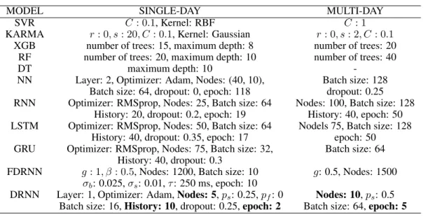
Table 2 shows the parameters of all the decoders for single- and multi-day analysis. The average performance of a small DRNN with a short history surpasses the other decoders’ in terms ofR2and
RMSE. Even the HL-DRNN’s results are comparable with the other larger recurrent models with longer histories. Figures 10, 11, and 12 show the single-day predictions of all the decoders on a sample
Table 2: Optimum parameters for different algorithms (Only differences are reported for multi-day)
MODEL SINGLE-DAY MULTI-DAY
SVR C: 0.1, Kernel: RBF C: 1
KARMA r: 0, s: 20, C: 0.1, Kernel: Gaussian r: 0, s: 2, C : 0.1
XGB number of trees: 15, maximum depth: 8 number of trees: 20
RF number of trees: 20, maximum depth: 10 number of trees: 40
DT maximum depth: 10
-NN Layer: 2, Optimizer: Adam, Nodes: (40, 10), Batch size: 128
Batch size: 64, dropout: 0, epoch: 118 dropout: 0.25
RNN Optimizer: RMSprop, Nodes: 25, Batch size: 64 Nodes: 100, Batch size: 128
History: 20, dropout: 0.2, epoch: 19 History: 40, epoch: 50
LSTM Optimizer: RMSprop, Nodes: 50, Batch size: 64 Nodels 75, Batch size: 128
History: 40, dropout: 0.35, epoch: 17 epoch: 50
GRU Optimizer: RMSprop, Nodes: 75, Batch size: 32, Batch size: 64
History: 40, dropout: 0.3
FDRNN g: 1, β: 0.5, Nodes: 1200, Batch size: 10 g: 0.5, Nodes: 1500
σb: 0.025,σs: 0.01,τ: 250 ms, epoch: 10
DRNN Layer: 1, Optimizer: Adam,Nodes: 5,ps: 0.25,pf: 0 Nodes: 10,ps: 0.5
Batch size: 16,History: 10, dropout: 0.25,epoch: 2 Batch size: 64,epoch: 5
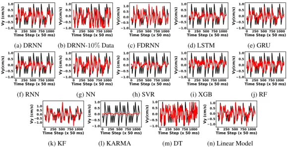
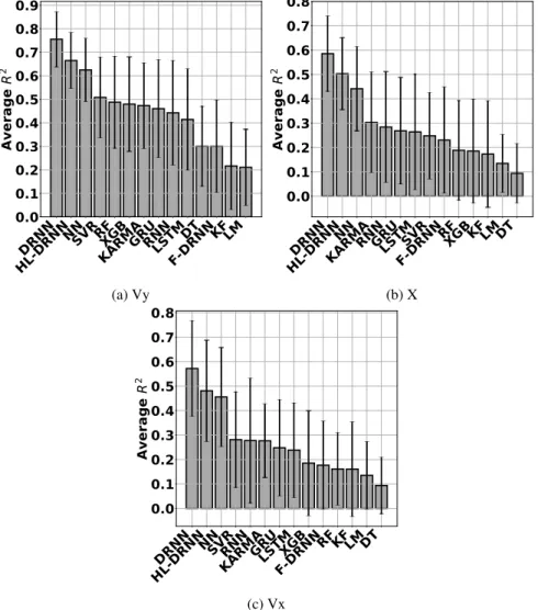
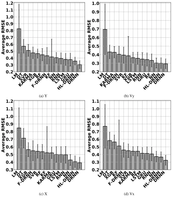
day for Vy, X, and Vx, respectively. Figures 13 and 14 show the average performance of all the decoders.
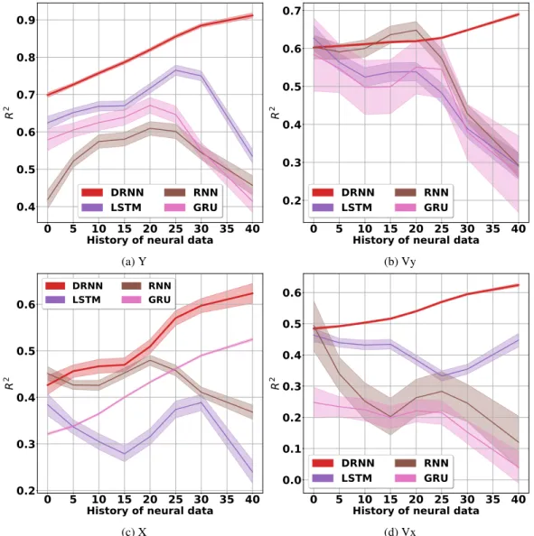
We do three more single-day analyses. First, we evaluate the effect of neural data history on the recurrent networks. Figures 15 and 16 show the performance of recurrent decoders versus history of neural data. The performance of other recurrent decoders drops, however, the DRNN’s performance is stable. Second, we evaluate the performance of the recurrent networks with different number of internal hidden nodes. Figures 17 and 18 show the performance of these decoders versus the number of hidden nodes. The DRNN’s performance has little changes when we add more nodes to the network. Moreover, it still performs superior to the other recurrent decoders. Third, we assess the stability of the recurrent networks to the amount of the single day’s training data. Figures 19 and 20 show that the DRNN’s performance is still better than the others. Moreover, it implies that the DRNN is a stable decoder and it works well even with less than10%single-day training data. Since we have only presented theR2values for Y-axis position in the body of the paper, we first present the corresponding RMSE values in figures 21, 22, 23, 24, and 25. These figures evaluate the average cross-day performance of the decoders by operating on different features, average multi-day performance of the DRNN on different features, average multi-day performance of the decoders operating on the MWT, effect of the used number of training days on the average performance of the decoders, and the effect of re-training on the DRNN’s long term stability and performance in different scenarios, respectively.
Subsequent figures present the equivalentR2and RMSE values for all the other kinematics. Figures
26 and 27 show the cross-day performance of the decoders. Figures 28 and 29 show the multi-day performance of the DRNN on the different features. Figures 30 and 31 show the performance of all the decoders operating on the MWT. Figures 24, 32, 34, 36, 38, 40, and 42 show the effect of number of training days on the performance of all the decoders. Finally, figures 25, 33, 35, 37, 39, 41, and 43 show the effect of re-training on the DRNN’s long term stability and performance in the different scenarios.
0 250 500 750 1000 Time Step (x 50 ms) 1.0 0.5 0.0 0.5 1.0 Vy (cm/s) (a) DRNN 0 250 500 750 1000 Time Step (x 50 ms) 1.0 0.5 0.0 0.5 1.0 Vy(cm/s) (b) DRNN-10%Data 0 250 500 750 1000 Time Step (x 50 ms) 1.0 0.5 0.0 0.5 1.0 Vy(cm/s) (c) FDRNN 0 250 500 750 1000 Time Step (x 50 ms) 1.0 0.5 0.0 0.5 1.0 Vy(cm/s) (d) LSTM 0 250 500 750 1000 Time Step (x 50 ms) 1.0 0.5 0.0 0.5 1.0 Vy(cm/s) (e) GRU 0 250 500 750 1000 Time Step (x 50 ms) 1.0 0.5 0.0 0.5 1.0 Vy(cm/s) (f) RNN 0 250 500 750 1000 Time Step (x 50 ms) 1.0 0.5 0.0 0.5 1.0 Vy (cm/s) (g) NN 0 250 500 750 1000 Time Step (x 50 ms) 1.0 0.5 0.0 0.5 1.0 Vy (cm/s) (h) SVR 0 250 500 750 1000 Time Step (x 50 ms) 1.0 0.5 0.0 0.5 1.0 Vy(cm/s) (i) XGB 0 250 500 750 1000 Time Step (x 50 ms) 1.0 0.5 0.0 0.5 1.0 Vy(cm/s) (j) RF 0 250 500 750 1000 Time Step (x 50 ms) 1.0 0.5 0.0 0.5 1.0 Vy (cm/s) (k) KF 0 250 500 750 1000 Time Step (x 50 ms) 1.0 0.5 0.0 0.5 1.0 Vy (cm/s) (l) KARMA 0 250 500 750 1000 Time Step (x 50 ms) 1.0 0.5 0.0 0.5 1.0 Vy(cm/s) (m) DT 0 250 500 750 1000 Time Step (x 50 ms) 1.0 0.5 0.0 0.5 1.0 Vy (cm/s) (n) Linear Model
Figure 10: Vy velocity regression of different algorithms on test data from the same day 2018-04-23: true target motion (black) and reconstruction (red).
0 250 500 750 1000 Time Step (x 50 ms) 1.0 0.5 0.0 0.5 1.0 X (cm) (a) DRNN 0 250 500 750 1000 Time Step (x 50 ms) 1.0 0.5 0.0 0.5 1.0 X(cm) (b) DRNN-10%Data 0 250 500 750 1000 Time Step (x 50 ms) 1.0 0.5 0.0 0.5 1.0 X(cm) (c) FDRNN 0 250 500 750 1000 Time Step (x 50 ms) 1.0 0.5 0.0 0.5 1.0 X(cm) (d) LSTM 0 250 500 750 1000 Time Step (x 50 ms) 1.0 0.5 0.0 0.5 1.0 X(cm) (e) GRU 0 250 500 750 1000 Time Step (x 50 ms) 1.0 0.5 0.0 0.5 1.0 X(cm) (f) RNN 0 250 500 750 1000 Time Step (x 50 ms) 1.0 0.5 0.0 0.5 1.0 X (cm) (g) NN 0 250 500 750 1000 Time Step (x 50 ms) 1.0 0.5 0.0 0.5 1.0 X (cm) (h) SVR 0 250 500 750 1000 Time Step (x 50 ms) 1.0 0.5 0.0 0.5 1.0 X(cm) (i) XGB 0 250 500 750 1000 Time Step (x 50 ms) 1.0 0.5 0.0 0.5 1.0 X(cm) (j) RF 0 250 500 750 1000 Time Step (x 50 ms) 1.0 0.5 0.0 0.5 1.0 X (cm) (k) KF 0 250 500 750 1000 Time Step (x 50 ms) 1.0 0.5 0.0 0.5 1.0 X (cm) (l) KARMA 0 250 500 750 1000 Time Step (x 50 ms) 1.0 0.5 0.0 0.5 1.0 X(cm) (m) DT 0 250 500 750 1000 Time Step (x 50 ms) 1.0 0.5 0.0 0.5 1.0 X (cm) (n) Linear Model
Figure 11: X position regression of different algorithms on test data from the same day 2018-04-23: true target motion (black) and reconstruction (red).
0 250 500 750 1000 Time Step (x 50 ms) 1.0 0.5 0.0 0.5 1.0 Vx (cm/s) (a) DRNN 0 250 500 750 1000 Time Step (x 50 ms) 1.0 0.5 0.0 0.5 1.0 Vx(cm/s) (b) DRNN-10%Data 0 250 500 750 1000 Time Step (x 50 ms) 1.0 0.5 0.0 0.5 1.0 Vx(cm/s) (c) FDRNN 0 250 500 750 1000 Time Step (x 50 ms) 1.0 0.5 0.0 0.5 1.0 Vx(cm/s) (d) LSTM 0 250 500 750 1000 Time Step (x 50 ms) 1.0 0.5 0.0 0.5 1.0 Vx(cm/s) (e) GRU 0 250 500 750 1000 Time Step (x 50 ms) 1.0 0.5 0.0 0.5 1.0 Vx(cm/s) (f) RNN 0 250 500 750 1000 Time Step (x 50 ms) 1.0 0.5 0.0 0.5 1.0 Vx (cm/s) (g) NN 0 250 500 750 1000 Time Step (x 50 ms) 1.0 0.5 0.0 0.5 1.0 Vx (cm/s) (h) SVR 0 250 500 750 1000 Time Step (x 50 ms) 1.0 0.5 0.0 0.5 1.0 Vx(cm/s) (i) XGB 0 250 500 750 1000 Time Step (x 50 ms) 1.0 0.5 0.0 0.5 1.0 Vx(cm/s) (j) RF 0 250 500 750 1000 Time Step (x 50 ms) 1.0 0.5 0.0 0.5 1.0 Vx (cm/s) (k) KF 0 250 500 750 1000 Time Step (x 50 ms) 1.0 0.5 0.0 0.5 1.0 Vx (cm/s) (l) KARMA 0 250 500 750 1000 Time Step (x 50 ms) 1.0 0.5 0.0 0.5 1.0 Vx(cm/s) (m) DT 0 250 500 750 1000 Time Step (x 50 ms) 1.0 0.5 0.0 0.5 1.0 Vx (cm/s) (n) Linear Model
Figure 12: Vx velocity regression of different algorithms on test data from the same day 2018-04-23: true target motion (black) and reconstruction (red).
DRNN
HL-DRNN
NNSVRRFXGB
KARMA
GRURNN
LSTM
DT
F-DRNN
KFLM
0.0
0.1
0.2
0.3
0.4
0.5
0.6
0.7
0.8
0.9
Av
er
ag
e
R
2 (a) VyDRNN
HL-DRNN
NN
KARMA
RNNGRU
LSTMSVR
F-DRNN
RFXGBKFLMDT
0.0
0.1
0.2
0.3
0.4
0.5
0.6
0.7
0.8
Av
er
ag
e
R
2 (b) XDRNN
HL-DRNN
NNSVRRNN
KARMA
GRU
LSTMXGB
F-DRNN
RFKFLMDT
0.0
0.1
0.2
0.3
0.4
0.5
0.6
0.7
0.8
Av
er
ag
e
R
2 (c) VxLMDTSVR
KARMA
XGBRF
F-DRNN
KFNNRNNLSTMGRU
HL-DRNN
DRNN
0.2
0.3
0.4
0.5
0.6
0.7
0.8
0.9
1.0
1.1
1.2
Average RMSE
(a) YLMDT
KARMA
F-DRNN
SVRKFXGBLSTMRNNGRURFNN
HL-DRNN
DRNN
0.2
0.3
0.4
0.5
0.6
0.7
0.8
0.9
1.0
Average RMSE
(b) VyLMDTXGB
F-DRNN
SVRRFKF
KARMA
GRU
LSTMRNNNN
HL-DRNN
DRNN
0.3
0.4
0.5
0.6
0.7
0.8
0.9
1.0
1.1
1.2
Average RMSE
(c) XLMDTXGBKF
F-DRNN
KARMA
SVR
RF
LSTMGRURNNNN
HL-DRNN
DRNN
0.2
0.3
0.4
0.5
0.6
0.7
0.8
0.9
1.0
1.1
Average RMSE
(d) Vx0 5 10 15 20 25 30 35 40
History of neural data
0.4
0.5
0.6
0.7
0.8
0.9
R
2DRNN
LSTM
RNN
GRU
(a) Y0 5 10 15 20 25 30 35 40
History of neural data
0.2
0.3
0.4
0.5
0.6
0.7
R
2DRNN
LSTM
RNN
GRU
(b) Vy0 5 10 15 20 25 30 35 40
History of neural data
0.2
0.3
0.4
0.5
0.6
R
2DRNN
LSTM
RNN
GRU
(c) X0 5 10 15 20 25 30 35 40
History of neural data
0.0
0.1
0.2
0.3
0.4
0.5
0.6
R
2DRNN
LSTM
RNN
GRU
(d) VxFigure 15: Performance of the recurrent networks versus the amount of single-day history of neural data.