Supplementary Material

(1)

Supplementary Material

A. Distributional Derivative of Stochastic Neuron

Before we prove the lemma3, we first introduce the chain rule of distributional derivative.

Lemma 6 (Grubb,2008) Letu∈ D0_{(Ω), we have}

1. (Chain Rule I)The distribution derivative ofv=u◦ffor anyf(x)∈ C1_{: Ω}0_→_Ω_{is given by}_Dv₌_Du∂f ∂x.

2. (Chain Rule II) The distribution derivative of v = f ◦ ufor any f(x) ∈ C1₍

R) withf0 bounded is given by

Dv=f0(u)Du.

Proof of Lemma3. Without loss of generality, we first consider1-dimension case. Given`(˜h) : R→R,ξ ∼ U(0,1),

˜ h: Ω→ {0,1}. For∀φ∈ C∞ 0 (Ω), we have Z φ(x)D`(˜h(x))dx=− Z φ0(x)`(x)dx = − Z 0 −∞ φ0(x)`(0)dx+ Z ∞ 0 φ0(x)`(1)dx = − φ(x) 0 −∞ `(0) +φ(x) ∞ 0 `(1) ! = (`(1)−`(0))φ(0)

where the last equation comes fromφ∈ C∞

0 (Ω). We obtain

D`(˜h) = (`(1)−`(0))δ(h) := ∆`(h).

We generalize the conclusion tol-dimension case with expectation overξ,i.e.,˜h(·, ξ) : Ω→ {0,1}l, we have the partial

distributional derivative fork-th coordinate as

DkE{ξi}li=1 h `(˜h(z, ξ))i = E{ξi}li=1 h Dk`(˜h(z, ξ)) i =E{ξi}li=1,i6=k h (`(˜h1_k)−`(˜h0_k))i.

Therefore, we have the distributional derivative w.r.t.W as

DE{ξi}li=1 h `(˜h(σ(W>x), ξ))i = E{ξi}li=1 h Dk`(˜h(σ(W>x), ξ)) i chain rule I = _E_{_ξ i}li=1 h D˜_h k`(˜h(σ(W >_x₎_{, ξ}₎₎_∇ Wσ(W>x) i = Eξ h ∆˜_h`(˜h(σ(W>x), ξ))σ(W>x)• 1−σ(W>x) x>i.

To derive the approximation of the distributional derivative, we exploit the mean value theorem and Taylor expansion.

Specifically, for a continuous and differential loss function`(·), there exists∈(0,1)

∂˜_h_k`(˜h)|˜_h_k₌=

h

∆_h˜`(˜h)

i

k.

Moreover, for general smooth functions, we rewrite the∂˜_h

Plugging into the distributional derivative estimator (7), we obtain a simple biased gradient estimator,

DWH˜(Θ;x)≈D˜WH˜(Θ;x) :=Eξ

h

∇˜_h`(˜h(σ(W>x), ξ))σ(W>x)•(1−σ(W>x))x>

i

(2)

B. Convergence of Distributional SGD

Lemma 7 (Ghadimi and Lan,2013) Under the assumption thatHisL-Lipschitz smooth and the variance of the stochastic distributional gradient (8) is bounded byσ2, the proposed distributional SGD outputs{Θi}

t i=1, t X i=1 γi− L 2γ 2 i E ∇Θ ˜ H(Θi) 2 6H˜(Θ0)−H˜(Θ ∗ ) + Lσ 2 2 t X i=1 γi2, whereΘt={Wt, Ut, βt, ρt}.

Proof of Theorem 5. Lemma7implies that by randomly sampling a search pointΘR with probabilityP(R = i) =

2γi−Lγ2i Pt i=12γi−Lγ2i whereγi∼ O 1/ √ tfrom trajectory{Θi} t i=1, we have E ∇Θ ˜ H(ΘR) 2 ∼ O ₁ √ t .

Lemma 8 Under the assumption that the variance of the approximate stochastic distributional gradient (10) is bounded byσ2_{, the proposed distributional SGD outputs}_{_Θ

i} t i=1such that t X i=1 γiE h (Θi−Θ∗)>∇˜ΘH˜(Θi) i 6 1₂ E h kΘ0−Θ∗k 2i + t X i=1 γi2σ 2 ! ,

whereΘ∗denotes the optimal solution.

Proof Denote the optimal solution asΘ∗, we have

kΘi+1−Θ∗k 2 = Θi−γi b ˜ ∇ΘH˜(Θi, xi)−Θ∗) 2 = kΘi−Θ∗k 2 +γ2_i b ˜ ∇ΘH˜(Θi, xi) 2 −2γi(Θi−Θ∗)>∇b˜ΘH˜(Θi, xi).

Taking expectation on both sides and denotingaj =kΘj−Θ∗k

2 , we have E[ai+1]6E[ai]−2γiE h (Θi−Θ∗)>∇˜ΘH˜(Θi) i +γ2_iσ2. Therefore, t X i=1 γiE h (Θi−Θ∗)>∇˜ΘH˜(Θi) i 6 1₂ E[a0] + t X i=1 γi2σ2 ! .

Theorem 9 Under the assumption that the variance of the approximate stochastic distributional gradient (10) is bounded by σ2_{, for the solution}_Θ

R sampled from the trajectory {Θi} t i=1 with probability P(R = i) = γi Pt i=1γi whereγi ∼ O 1/√t , we have E h (ΘR−Θ ∗ )>∇˜ΘH˜(ΘR) i ∼ O 1 √ t ,

whereΘ∗denotes the optimal solution.

Proof The lemma 8 implies by randomly sampling a search point ΘR with probabilityP(R = i) = Ptγi

i=1γi where

γi∼ O 1/ √

t

from trajectory{Θi}t_i₌₁, we have

E h (ΘR−Θ∗)>∇˜ΘH˜(ΘR) i 6 E h kΘ0−Θ∗k 2i +Pt i=1γ 2 iσ2 2Pt i=1γi ∼ O ₁ √ t .

(3)

C. More Experiments

C.1. Convergence of Distributional SGD and Reconstruction Error Comparison

0 0.5 1 1.5 2 2.5

number of samples visited #106 5 10 15 20 25 30 L2 reconstruction error

MNIST L2 reconstruction error

8 bits ITQ 16 bits ITQ 32 bits ITQ 64 bits ITQ 8 bits SGH 16 bits SGH 32 bits SGH 64 bits SGH 0 0.5 1 1.5 2 2.5

number of samples visited #106 0.4 0.5 0.6 0.7 0.8 0.9 1 1.1 1.2 L2 reconstruction error

GIST L2 reconstruction error

8 bits ITQ 16 bits ITQ 32 bits ITQ 64 bits ITQ 8 bits SGH 16 bits SGH 32 bits SGH 64 bits SGH

(a)MNIST (b)GIST-1M

Figure 4: L2 reconstruction error convergence onMNISTandGIST-1Mof ITQ and SGH over the course of training with

varying of the length of the bits (8, 16, 32, 64, respectively). The x-axis represents the number of examples seen by the training algorithm. For ITQ, it sees the training dataset once in one iteration.

We shows the reconstruction error comparison between ITQ and SGH onMNISTandGIST-1Min Figure4. The results

are similar to the performance on SIFT-1M. Because SGH optimizes a more expressive objective than ITQ (without

orthogonality) and do not use alternating optimization, it find better solution with lower reconstruction error.

C.2. Training Time Comparison

8 16 32 64

bits of hashing codes

0 200 400 600 800 1000 1200

Training Time (sec)

MNIST Training Time

BA SGH

8 16 32 64

bits of hashing codes

0 0.5 1 1.5 2

Training Time (sec)

#104 GIST Training Time

BA SGH

(a)MNIST (b)GIST-1M

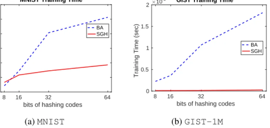
Figure 5: Training time comparison between BA and SGH onMNISTandGIST-1M.

We shows the training time comparison between BA and SGH on MNISTandGIST-1Min Figure5. The results are

similar to the performance onSIFT-1M. The proposed distributional SGD learns the model much faster.

C.3. More Evaluation on L2NNS Retrieval Tasks

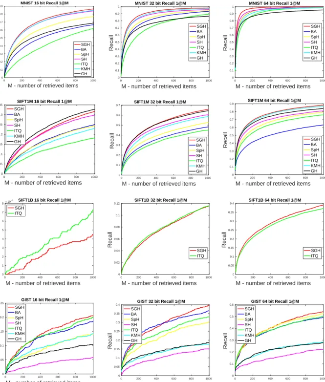
We also use different RecallK@N to evaluate the performances of our algorithm and the competitors. We first evaluated

the performance of the algorithms with Recall 1@N in Figure6. This is an easier task comparing toK= 10. Under such

measure, the proposed SGH still achieve the state-of-the-art performance.

In Figure7, we setK, N= 100and plot the recall by varying the length of the bits onMNIST,SIFT-1M, andGIST-1M.

This is to show the effects of length of bits in different baselines. Similar to the Recall10@N, the proposed algorithm still consistently achieves the state-of-the-art performance under such evaluation measure.

(4)

D. Stochastic Generative Hashing For Maximum Inner Product Search

In Maximum Inner Product Search (MIPS) problem, we evaluate the similarity in terms of inner product which can avoid

the scaling issue,i.e., the length of the samples in reference dataset and the queries may vary. The proposed model can also

be applied to the MIPS problem. In fact, the Gaussian reconstruction model also preserve the inner product neighborhoods.

Denote the asymmetric inner product asx>U hy, we claim

Proposition 10 The Gaussian reconstruction error is a surrogate for asymmetric inner product preservation.

Proof We evaluate the difference between inner product and the asymmetric inner product,

kx>y−x>U>hyk2=kx> y−U>hy

k26kxk2ky−U>hyk2,

which means minimizing the Gaussian reconstruction,i.e.,−logp(x|h), error will also lead to asymmetric inner product

preservation.

We emphasize that our method is designed for hashing problems primarily. Although it can be used for MIPS problem, it is different from the product quantization and its variants whose distance are calculated based on lookup table. The proposed distributional SGD can be extended to quantization. This is out of the scope of this paper, and we will leave it as the future work.

D.1. MIPS Retrieval Comparison

To evaluate the performance of the proposed SGH on MIPS problem, we tested the algorithm onWORD2VECdataset for

MIPS task. Besides the hashing baselines, since KMH is the Hamming distance generalization of PQ, we replace the KMH

with product quantization (Jegou et al.,2011). We trained the SGH with 71,291 samples and evaluated the performance

with 10,000 query. Similarly, we vary the length of binary codes from16,32to64, and evaluate the performance by Recall

10@N. We calculated the ground-truth via retrieval through the original inner product. The performances are illustrated

in Figure8. The proposed algorithm outperforms the competitors significantly, demonstrating the proposed SGH is also

applicable to MIPS task.

E. Generalization

We generalize the basic model to translation and scale invariant extension, semi-supervised extension, as well as coding

withh∈ {−1,1}l_.

E.1. Translation and Scale Invariant Reduced-MRFs

As we known, the data may not zero-mean, and the scale of each sample in dataset can be totally different. To eliminate the translation and scale effects, we extend the basic model to translation and scale invariant reduced-MRFs by introducing

parameterαto separate the translation effect and the latent variablezto model the scale effect in each samplex, therefore,

the potential function becomes

E(x, h, z) =−β>_h₊ 1

2ρ2(x−α−U

>₍_z_·_h₎₎>₍_x₋_α₋_U>₍_z_·_h₎₎_, ₍₁₅₎

where·denotes element-wise product,α∈_Rd_and_z_∈

Rl. Comparing to (2), we replaceU>hwithU>(z·h) +αso that

the translation and scale effects in both dimension and sample are modeled explicitly.

We treat theαas parameters andzas latent variable. Assume the independence in posterior for computational efficiency,

we approximate the posteriorp(z, h|x)withq(h|x;Wh)q(z|x;Wz), whereWh, Wzdenotes the parameters in the posterior

approximation. With similar derivation, we obtain the learning objective as

max U,α,β,ρ;Wh,Wz 1 N N X i=1

Eq(h|xi)q(z|xi)[−E(x, h, z)−logq(h|xi)−logq(z|xi)]. (16)

Obviously, the proposed distributional SGD is still applicable to this optimization.

E.2. Semi-supervised Extension

Although we only focus on learning the hash function in unsupervised setting, the proposed model can be easily extended to

(5)

we are provided the (partial) supervision information for some pairs of data,i.e.,S={xi, xi, yij}Mi,j, where

yij=

(

1 ifxi∈ N N(xj)orxj∈ N N(xi)

0 o.w. ,

andN N(x)stands for the set of nearest neighbors ofx. Besides the original Gaussian reconstruction model in the basic

model in (2), we introduce the pairwise modelp(yij|hi, hj) = B(σ(h>i hj))into the framework, which results the joint

distribution overx, y, has

p(xi, xj, hi, hj, yij) =p(xi|hi)p(xj|hj)p(hi)p(hj)p(yij|hi, hj)1S(ij),

where1S(ij)is an indicator that outputs1when(xi, xj)∈ S, otherwise0. Plug the extended model into the Helmholtz

free energy, we have the learning objective as,

Obviously, the proposed distributional SGD is still applicable to the semi-supervised extension.

E.3.{±1}-Binary Coding

In the main text, we mainly focus on coding with{0,1}. In fact, the proposed model is applicable to coding with{−1,1}

with minor modification. Moreover, the proposed distributional SGD is still applicable. We only discuss the basic model here, the model can also be extended to scale-invariant and semi-supervised variants.

If we seth∈ {−1,1}l_{, the potential function of basic reduced-MRFs (}₂_{) does not have any change,}_i.e._,

E(x, h) =−β>h+ 1 2ρ2 x

>_x₊_h>_U>_{U h}₋₂_x>_{U h}

. (17)

We need to modify the parametrization ofq(h|x)as

q(h|x) = l Y i=1 σ(wi>x) 1+hi 2 ₁−_σ₍_w> i x) 1−hi 2 _. ₍₁₈₎

Therefore, the stochastic neuron becomes

f(z, ξ) :=

(

1 ifσ(z)_>ξ −1 ifσ(z)< ξ .

With similar derivation, we have the distributional derivative of the objective w.r.t.W as

∇WLsn=Eξ ∆f`(f(z, ξ))∇zσ(z)x> , (19) where[∆f`(f(z, ξ))]_k=`(fk1)−`(f −1

k ). Furthermore, we have a similar biased gradient estimator as

˜ ∇WLsn=Eξ ∇f`(f(z, ξ))∇zσ(z)x> . (20)

(6)

0 200 400 600 800 1000

M - number of retrieved items

0 0.1 0.2 0.3 0.4 0.5 0.6 0.7 0.8 0.9 Recall

MNIST 16 bit Recall 1@M

SGH BA SpH SH ITQ KMH GH 0 200 400 600 800 1000 M - number of retrieved items 0 0.1 0.2 0.3 0.4 0.5 0.6 0.7 0.8 0.9 1 Recall

SGH BA SpH SH ITQ KMH GH 0 200 400 600 800 1000

0 0.05 0.1 0.15 0.2 0.25 0.3 0.35 Recall

SIFT1M 16 bit Recall 1@M

SGH BA SpH SH ITQ KMH GH 0 200 400 600 800 1000 M - number of retrieved items 0 0.1 0.2 0.3 0.4 0.5 0.6 0.7 Recall

SGH BA SpH SH ITQ KMH GH 0 200 400 600 800 1000 M - number of retrieved items 0 0.1 0.2 0.3 0.4 0.5 0.6 0.7 0.8 0.9 Recall

SGH BA SpH SH ITQ KMH GH 0 200 400 600 800 1000 M - number of retrieved items 0 1 2 3 4 5 6 7 8 Recall

#10-3 SIFT1B 16 bit Recall 1@M

SGH ITQ

0 200 400 600 800 1000 M - number of retrieved items 0 0.02 0.04 0.06 0.08 0.1 0.12 Recall

SIFT1B 32 bit Recall 1@M

SGH ITQ

0 200 400 600 800 1000 M - number of retrieved items 0 0.05 0.1 0.15 0.2 0.25 0.3 0.35 0.4 Recall

SIFT1B 64 bit Recall 1@M

SGH ITQ

0 200 400 600 800 1000 M - number of retrieved items 0 0.05 0.1 0.15 0.2 0.25 Recall

GIST 16 bit Recall 1@M

SGH BA SpH SH ITQ KMH GH 0 200 400 600 800 1000 M - number of retrieved items 0 0.05 0.1 0.15 0.2 0.25 0.3 0.35 0.4 Recall

SGH BA SpH SH ITQ KMH GH 0 200 400 600 800 1000 M - number of retrieved items 0 0.1 0.2 0.3 0.4 0.5 0.6 Recall

SGH BA SpH SH ITQ KMH GH

Figure 6: L2NNS comparison onMNIST,SIFT-1M,SIFT-1B, andGIST-1Mwith the length of binary bits from16to

(7)

8 16 32 64

bits of hashing code

0 0.1 0.2 0.3 0.4 0.5 Recall 100@100 SGH BA SpH SH ITQ KMH GH 8 16 32 64

0 0.05 0.1 0.15 0.2 0.25 Recall 100@100 SGH BA SpH SH ITQ KMH GH 8 16 32 64

0 0.02 0.04 0.06 0.08 Recall 100@100 SGH BA SpH SH ITQ KMH GH

(a) L2NNS onMNIST (b) L2NNS onSIFT-1M (c) L2NNS onGIST-1M

Figure 7: L2NNS comparison onMNIST,SIFT-1M, andGIST-1Mwith Recall 100@100 for the length of bits from8to

64.

0 200 400 600 800 1000 M - number of retrieved items 0 0.05 0.1 0.15 0.2 0.25 0.3 0.35 0.4 0.45 Recall

WORD2VEC 16 bit Recall 10@M

SGH BA SpH SH ITQ PQ 0 200 400 600 800 1000 M - number of retrieved items 0 0.1 0.2 0.3 0.4 0.5 0.6 0.7 Recall

SGH BA SpH SH ITQ PQ 0 200 400 600 800 1000

0 0.1 0.2 0.3 0.4 0.5 0.6 0.7 0.8 Recall

SGH BA SpH SH ITQ PQ

Figure 8: MIPS comparison onWORD2VECwith the length of binary bits from16to64. We evaluate the performance with