Biology Faculty Publications
Department of Biology
2015
Detecting Conserved Protein Complexes Using a
Dividing-and-Matching Algorithm and Unequally
Lenient Criteria for Network Comparison
Yi Pan
Georgia State University, [email protected]
Wei Peng
Central South University
Jianxin Wang
Central South University, [email protected]
Fangxiang Wu
University of Saskatchewan, [email protected]
Follow this and additional works at:
http://scholarworks.gsu.edu/biology_facpub
Part of the
Biology Commons
This Article is brought to you for free and open access by the Department of Biology at ScholarWorks @ Georgia State University. It has been accepted for inclusion in Biology Faculty Publications by an authorized administrator of ScholarWorks @ Georgia State University. For more information, please [email protected].
Recommended Citation
Pan, Yi; Peng, Wei; Wang, Jianxin; and Wu, Fangxiang, "Detecting Conserved Protein Complexes Using a Dividing-and-Matching Algorithm and Unequally Lenient Criteria for Network Comparison" (2015).Biology Faculty Publications.Paper 5.
RESEARCH
Detecting conserved protein complexes
using a dividing-and-matching algorithm
and unequally lenient criteria for network
comparison
Wei Peng
1,2, Jianxin Wang
1*, Fangxiang Wu
3and Pan Yi
4Abstract
The increase of protein–protein interaction (PPI) data of different species makes it possible to identify common subnetworks (conserved protein complexes) across species via local alignment of their PPI networks, which benefits us to study biological evolution. Local alignment algorithms compare PPI network of different species at both protein sequence and network structure levels. For computational and biological reasons, it is hard to find common subnet-works with strict similar topology from two input PPI netsubnet-works. Consequently some methods introduce less strict criteria for topological similarity. However those methods fail to consider the differences of the two input networks and adopt equally lenient criteria on them. In this work, a new dividing-and-matching-based method, namely UEDA-MAlign is proposed to detect conserved protein complexes. This method firstly uses known protein complexes or computational methods to divide one of the two input PPI networks into subnetworks and then maps the proteins in these subnetworks to the other PPI network to get their homologous proteins. After that, UEDAMAlign conducts unequally lenient criteria on the two input networks to find common connected components from the proteins in the subnetworks and their homologous proteins in the other network. We carry out network alignments between S. cerevisiae and D. melanogaster, H. sapiens and D. melanogaster, respectively. Comparisons are made between other six existing methods and UEDAMAlign. The experimental results show that UEDAMAlign outperforms other existing methods in recovering conserved protein complexes that both match well with known protein complexes and have similar functions.
Keywords: Network alignment, Local network alignment, Conserved protein complexes, PPI networks
© 2015 Peng et al. This article is distributed under the terms of the Creative Commons Attribution 4.0 International License (http://creativecommons.org/licenses/by/4.0/), which permits unrestricted use, distribution, and reproduction in any medium, provided you give appropriate credit to the original author(s) and the source, provide a link to the Creative Commons license, and indicate if changes were made. The Creative Commons Public Domain Dedication waiver (http://creativecommons.org/ publicdomain/zero/1.0/) applies to the data made available in this article, unless otherwise stated.
Background
The majority of biological processes are not carried out by a single protein alone but by a group of proteins which physically interact with each other to form protein com-plexes. It is believed that protein complexes are the build-ing blocks of the cellular machinery and protein–protein interaction (PPI) networks evolve at module level [1]. Consequently, identifying protein complexes of a sin-gle species plays a significant role in understanding the
underlying mechanism of cellular function, and iden-tifying protein complexes conserved across difference species are helpful for studying biological evolution. Recently, some computational methods have been pro-posed to identify protein complexes from a single PPI network [2–9]. The underlying hypothesis behind these methods is that a protein complex corresponds to a dense subgraph or cluster of a single PPI network. Meanwhile, some computational methods have been introduced to identify the common subnetworks (conserved functional modules) across species by comparatively analyzing PPI networks of different species.
In contrast to traditional sequence-comparison-based methods, network-comparison-based methods provide
Open Access
*Correspondence: [email protected]
1 The School of Information Science and Engineering, Central South University, Changsha, Hunan, People’s Republic of China
a new view of studying biological evolution, which con-siders two proteins conserved across species if they have both similar sequences and similar interactive pat-terns. The two proteins (homologous protein pairs) that are from two different PPI networks and have similar sequences are believed to have similar interactive pat-terns if their neighbors in corresponding PPI networks also have similar sequences. These network-comparison-based methods define the problem as network alignment. In context of biology, there are two challenges exist in PPI network alignment. The one is there exist many-to-many mappings between proteins of different species, which is the result of biological evolution, such as gene duplica-tion [10]. The other is few strict meaning of conserved interactive patterns exist due to emergence or elimina-tion of interacelimina-tions in the course of evoluelimina-tion.
According to differences in the ways to deal with many-to-many mapping, network alignment can be classified into two categories: global alignment and local align-ment [11]. The aim of global alignment is to find one-to-one optimal mappings between proteins of two PPI networks. Global alignment can help us to understand variations between species and be used to detect func-tions of orthologs and construct phylogenetic relation-ships. There are also some global alignment methods [12] adopt some clustering methods to detect conserved sub-networks based on the best mappings between the nodes from different PPI networks. However, these methods ignore the facts that there exist duplications of interact-ing proteins and even whole complexes in a sinteract-ingle spe-cies. Previous studies observe that a significant fraction of complexes in S. cerevisiae (yeast) share strong similar-ity with each other [13]. By contrast, local alignment is utilized to detect pathways or protein complexes that are conserved across multiple species. There exist many-to-many mappings between proteins of two PPI networks. Note that there are also other global or local alignment methods [14–17] incorporate some biological informa-tion, such as functional annotainforma-tion, protein structure information, protein domain information to find truly homologous proteins and reduce the impacts of many-to-many mappings. This work focuses on local align-ment, whose goal is to find conserved complexes across different species only depending on sequence and topo-logical similarity.
Up to now, many local alignment methods have been proposed to detect conserved protein complexes. Gen-erally, there are two types of local alignment methods: alignment-graph-based method and dividing-and-match-ing-based method. The basic idea of alignment-graph-based method is that false positive protein interactions are rare possible to duplicate in other species and merging two PPI networks being compared according
homologous mappings between proteins can filter false positive protein interactions. Alignment-graph-based methods [18–21] usually take two steps to identify con-served complexes. Firstly, a weighted alignment graph is built from two input PPI networks. Each node of the graph is composed of a pair of homologous proteins, one from each network. Each edge of the graph is weighed by certain methods that account for the degree to which an interaction in one PPI network is conserved across spe-cies. After that, some clustering methods are adopted to detect conserved protein complexes from the weighted alignment graph. Those existing alignment-graph-based methods differ in the strategies taken to construct align-ment graph and to clustering the alignalign-ment graph. Divid-ing-and-matching-based method is an alternatively way of finding conserved complexes, which firstly uses known protein complexes or computational methods to divide one of the two input PPI networks into subnetworks and then maps the proteins in these subnetworks to the other PPI network [22–25]. The motivation underlying this kind of methods is to investigate how those protein com-plexes that are experimentally or computationally identi-fied from a single species are conserved across species. In recent years, there are available know protein complexes of some species, such as yeast and human, and some computational methods that have good performance of detecting protein complexes from the PPI network of single species [2, 26–30]. All of this make it pressing to design an effective dividing-and-matching-based method to identify conserved protein complexes.
To overcome the challenge that there are few strict meaning of conserved interactions across species, both alignment-graph-based methods and dividing-and-matching-based methods introduce less restric-tive definition of conserved interactions in the course of comparison. As for alignment-graph-based method, some methods, such as Network-Blast [18], Network-Path [31] and Mawish [19], introduce edges in align-ment graph if a pair of proteins in one networks is directly connected while their homologous proteins in the other network are indirectly connected. How-ever PHUNKE [20] cancels the requirement of indi-rect connection between homologous proteins in the other network and connects two nodes in alignment graph if there is at least a pair of proteins in one net-work is directly connected. AlignNemo [17] adopts less restrict criterion and constructs edges in align-ment graph if a least a pair of proteins in one PPI net-work is directly or indirectly connected. NetAligner [32] adds edges between node pair in alignment graph at a distance greater than 2 and tolerates gaps and mis-match of any length. As for dividing-and-mis-matching- dividing-and-matching-based method, Manikandan et al. [33] have proposed a
Match-and-Split algorithm which matches proteins of two networks according to a local matching criterion and splits the whole networks into connected compo-nents. This process is recursively implemented on those components and finally outputs conserved complexes. Luqman and Karp [24] have introduced Produles which uses PageRank-Nibble [34] algorithm to partition one of the two input networks and maps these subnetworks to the other network. After that, a local extension is imple-mented to detect the connected components that con-sist of the homologous proteins in the other network. According to those connected components, the subnet-works are refined and the connected parts in them are extracted as conserved protein complexes. Obviously, Match-and-Split and Produles algorithm do not match the two networks exactly in their graph structure. How-ever, they only take direct neighbors into account when implementing local alignment, which is so rigid that very few conserved protein complexes are identified. With respect to this, DAMAlign [25] is proposed in our previous work, which takes both dividing-and-matching strategies and the same lenient criteria as AlignNemo to locally extend a pair of homologous protein pairs. That is, in the course of finding common connected compo-nents, DAMAlign recruits a pair of homologous pro-teins if there is at least one path of length not larger than 2 to connect one of node in the homologous protein pair in its corresponding network. The comparisons made by previous studies show that AlignNemo, AlignMCL [21] and DAMAlign succeed in detecting more conserved complexes than previous methods [18, 19], such as Mawish, NetworkBlast,PHUNKEE and Produles. The reason may be considering indirectly connected node pairs in one network is robust against missing interac-tions in original network. Although NetAligner employs more lax criteria to introduce conserved interactions, it also yields a lot of false positive conserved interactions, which reduces its performance of detecting conserved complexes.
In spite of that previous researchers have done great efforts to improve the performance of their methods by introducing less strict criteria to find conserved interactions, few of them consider the difference of the two input networks and adopt equally lenient crite-ria on them. In fact, there exist differences between PPI networks of different species in their structures and topologies. The distance between proteins that have homologous proteins in the other PPI network may vary with species. Therefore, in this work, we propose a new dividing-and-matching method named by UEDAMA-lign to detect conserved protein complexes via local network alignment. UEDAMAlign, similar to previous dividing-and-matching methods, such as Produles and
DAMAlign, partitions one of PPI network into subnet-works and then maps these subnetsubnet-works to the other PPI network to find common connected components. In contrast to previous dividing-and-matching methods, UEDAMAlign implements unequal criteria on the two networks to find common connected components with respect to the structural and topological differences of the two networks. That is UEDAMAlign locally extends a pair of homologous proteins if there is a path of length not larger than l to connect the homologous protein in the PPI network one or a path of length not larger than r to connect the homologous protein in the other net-work. To evaluate the effectiveness of UEDAMAlign, We carry out network alignment between S. cerevisiae and D. melanogaster, H. sapiens and D. melanogaster, respectively. Comparisons are made between other six existing methods and UEDAMAlign whose parameters l and r are both set to 2. The experimental results show that When UEDAMAlign takes the same lenient criteria as AlignNemo and DAMAlign do, it is superior to other existing methods because it can detect conserved pro-tein complexes that both match well with known propro-tein complexes and have similar functions. Finally, we discuss the effect of parameters l and r on the performance of UEDAMAlign.
Methods
The detection process of UEDAMAlign is broadly divided into four steps. At the beginning, several random walking steps are unequally taken on the two input PPI networks to detect some potential mappings between proteins of the two networks. After that, one of the two PPI networks is divided by known protein complexes or computational methods. Then proteins in those subnet-works are mapped to the other PPI network to find their homologous proteins and the connected components of those homologous proteins are extracted from the other PPI networks by using a heuristic approach. The final step of UEDAMAlign is to filter out the predicted con-served complexes that are highly overlapping with others.
Exploring potential mappings between proteins of two species
In network alignment, the homologous mappings between the proteins of two different PPI networks can be inferred from their sequence-based similarity. Those proteins with similar sequences are most likely to evolve from a common ancestor and thus have simi-lar functions. Moreover, interactive proteins of a single species tend to share common functions. Therefore, we assume that the protein and its neighbors in a single PPI network should map to a common protein in the other PPI network. Since proteins are most likely to
share functions not only with their direct neighbors but also with their indirect neighbors, and even with their level k neighbors, some potential mappings between proteins of two species can be inferred from their direct, indirect or level k neighbors. Furthermore, the level of neighbors with which a protein tend to share functions varies with species due to the structural and topological difference of their PPI networks. Hence, we should infer potential protein–protein mappings from unequal level of neighbors for different species. In this work, we adopt an unbalanced Bi-random walk algorithm to find potential mapping between proteins of two species. This method has also been used in our previous study [35] that gets protein-function asso-ciations by walking different number of steps in PPI network and functional interrelationship network. To formally define our method, some variables are intro-duced in advance.
Let P(N*N) and H(M*M) be adjacent matrixes of two input PPI networks respectively. P(N*N) is row-normal-ized and H(M*M) is column-normalized. The element p(i, j) of matrix P(N*N) and h(i, j) of matrix H(M*M) is defined as follows.
where degree(i) denotes sum of interactions of node i . Let matrix A(N*M) represent known protein–pro-tein mappings measured by sequence-based similari-ties. Its element a(i,j) is 1, if there exists an mapping between protein i of one species and protein j of the other one, 0 otherwise. R(N*M) denotes the final protein–protein mappings. The value of its element r(i,j) represents the probability that protein i will be mapped to protein j.
Given matrix P, H and A, we want to calculate matrix R. Since proteins and their level k neighbors in one PPI net-work may map to the same proteins in the counterpart network, several random walk steps are taken on the two PPI networks, respectively. At each walking step, multi-plying P on the left and H on the right respectively can detect some potential protein–protein mappings (Eqs. 3, 4). Then the weighted average of the multiply results updates matrix R (Eq. 5). Consider the difference of the two input networks, the level of neighbors from which the proteins infer mapping information should be dif-ferent. To address this problem, two parameters (l and r) are adopted to control maximal iteration steps in the two networks. Mathematically, the process can be expressed as Algorithm 1. (1) p(i,j)= = 1 degree(i) if degree(i) >0 0 otherwise . (2) h(i,j)= = 1 degree(j) if degree(j) >0 0 otherwise .
where t (=1, 2, . . .) represents the walking steps. Matrix A storing known protein–protein mappings can regu-late the iteration process. The parameter α(0< α <1) is used to adjust the weight of regulation of network and of prior knowledge stored in Matrix A (in this work, α is set to 0.5). p or h are indicators which are 1 if the
number of walk steps on PPI network One or Two are less than their thresholds (l or r), respectively, 0 oth-erwise. ISORank [11] adopts similar strategy to obtain potential mappings between proteins of two different PPI networks and computes their global network alignment. In ISORank, however, random walks are taken simulta-neously on the two networks until the global networks. Actually, ISORank treats the two networks equally. How-ever, Our work separately takes random walks on two networks, which walks only several steps (t is set to 1, 2, . . .) and is convenient for controlling different walk-ing steps taken on the two networks accordwalk-ing to their difference in topology and structure. Consequently, our method is more flexible to get protein–protein mappings between two PPI networks.
Detecting conserved protein complexes from PPI networks
The basic idea of UEDAMAlign is first dividing PPI net-works into small subnetnet-works and then mapping pro-teins of subnetworks to the other PPI network. Many computational methods, such as Coach [36], MCL [37, 38], CMC [39], CFinder [40] and so on, have been pro-posed to detect protein complexes form a single PPI network and achieve good performance. Moreover, biological experiments have been implemented on sev-eral species and the data of known protein complexes is available. Consequently those known protein com-plexes or those predicted by computational methods can be conveniently used as partition of a PPI network. The main challenge of UEDAMAlign lies in mapping proteins in subnetworks of a PPI network to the other one in order to find common connected components. In the course of finding common connected components,
Algorithm 1Finding potential mappings
1:Input:MatrixP,H,Aparameterα,iteration stepsl,r; 2:Output:predicted association matrixR;
3:R0=A= A sum(A) 4:for(t= 1to max(l,r))do 5: λp=λh= 0; 6: if(t < l)then 7: Rt
p=αP∗Rt−1+ (1−α)A (3) //P P I network One
8: λp= 1 9: end if 10: if(t<r)then 11: Rt h=αRt− 1 ∗H+ (1−α)A (4) //P P I network T wo 12: λh= 1 13: end if 14: Rt= (λp∗Rt
p+λh∗Rth)/(λp+λh) (5) //M erge two results
15: end for
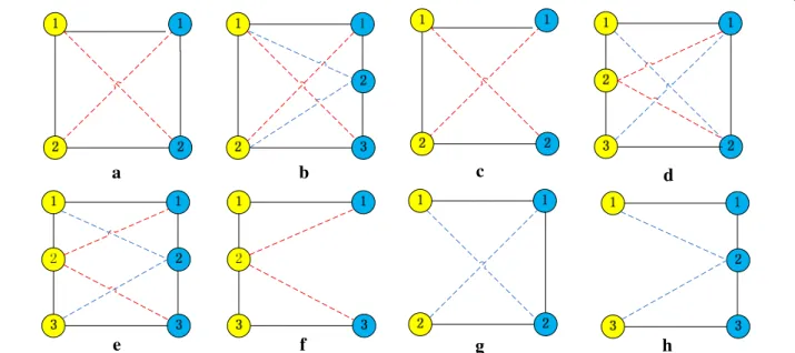
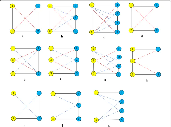
UEDAMAlign adopts unequally lenient criteria to extend a pair of homologous proteins. The span dis-tance of a protein pair in a single network is unequal with respect to the difference of input PPI networks, which is determined by inputting parameters l and r. For example, when taking the same lenient criteria as AlignNemo and DAMAlign do, UEDAMAlign absorbs a pair of homologous proteins into its predicted con-served protein complexes if at least one of protein in the homologous protein pair connects to the proteins in the predicted conserved protein complexes through a path of length not larger than 2. In this case, parameters l and r are set to 2. When parameters l and r are set to 2 and 3 respectively, UEDAMAlign locally extends a pair of homologous proteins if there exists a path of length not larger than 2 to connect the node in the homolo-gous protein pair in PPI network one or a path of length not larger than 3 to connect the node in the homolo-gous protein pair in PPI network two. Figure 1 shows eight cases of connectivity in conserved protein com-plexes from two different PPI networks when l and r are set to 2. Figure 2 shows eleven cases of connectivity in conserved protein complexes from two different PPI networks when l and r are set to 2 and 3 respectively. The nodes with different color come from different PPI networks. The full lines connecting two different color nodes represent their known homologous mappings. The dot lines represent artificial homologous mappings detected by unbalanced Bi-random walk algorithm. The
full lines connecting the same color nodes represent their interactions.
Given k subnetworks p1,p2,. . .pk extracted from PPI
network P(N*N), the other PPI network H(M*M), known protein–protein mapping matrix A(N*M), parameter l, r and a constructed mapping matrix R(N*M), UEDAMA-lign proceeds as follows:
Step 1: In this step, we aim to extract the proteins from an input subnetwork that both have homologs in the other PPI network and are connected through at least one path of length not larger than a threshold. The threshold is set to l and r for network P and H, respec-tively. Given ModuleOne and ModuleTwo store con-served protein complexes induced from PPI network P and H respectively. Start from an arbitrarily node of subnetwork pi(i=1, 2,. . .k), find its homologous pro-teins in H, which are homologous to both the node and its neighbors in the input subnetwork pi according to the
matrix R. Put the neighbors into ModuleOne if they sat-isfy one of following conditions:
1. There exists at least one real homologous mapping between the shared homologous proteins and the nodes or its neighbors
2. There exist two different homologous proteins shared by the node and its neighbors but also the two dif-ferent homologous proteins are really matched with two proteins other than the node and its neighbors in input subnetwork pi.
b
c
d
g
h
f
a
e
Figure 1 Eight cases (a–h) of connectivity in conserved protein complexes from two different PPI networks when UEDAMAlign adopts the same lenient criteria as AlignNemo does to extend a pair of homologous proteins. The nodes with different color come from different PPI networks. The full lines connecting two different color nodes represent their known homologous mappings. The dot lines represent artificial homologous mappings by a unbalanced Bi-random walk algorithm. The full lines connecting the same color nodes represent their interactions.
Since there are some artificial mappings in matrix R, only those real homologous proteins are put into Mod-uleTwo. The real homologous mappings are stored in Matrix A. Then start again from the neighbors, repeat the process in step 1 until no more nodes in subnetworks pi
can been put into ModuleOne.
Step 2: The aim of step 2 is to refine ModuleTwo by reducing many-to-many homologous mappings. Each node in ModuleTwo is assigned a weight, which is defined as sum of mapping values in matrix R between the node and its counterpart in ModuleOne. Con-nected components from proteins in ModuleTwo are deduced by searching both their direct neighbors and up to level l or r neighbors (level l neighbors for sub-networks from network P, level r neighbors for subnet-works from H). For the components that consist of at
least two nodes, their counterparts in ModuleOne are regard as being covered. Exclude components with one node from ModuleTwo if their counterparts in Module-One have been covered. Otherwise, keep the one with high weight .
Step 3: In this step, we will handle the case that the node of input subnetwork are isolated but their homolo-gous proteins have connections with protein in Modu-leTwo. For example, when the parameters l and r are set to 2, steps 1 and 2 can cover the case of Figure 1a–f. In step 3, we consider the case of Figure 1g, h. When the parameters l and r are set to 2 and 3, respectively, steps 1 and 2 can cover the case of Figure 2a–h. In step 3, we con-sider the case of Figure 2i–k. Check the rest of proteins in subnetworks pi but not in ModuleOne. Attach them
to ModuleOne if their counterparts (true homologous
a b d f e i j k c g h
Figure 2 Eleven cases (a–k) of connectivity in conserved protein complexes from two different PPI networks, when parameters l and r are set to 2 and 3 in the course of extending a pair of homologous proteins. The nodes with different color come from different PPI networks. The full lines connecting two different color nodes represent their known homologous mappings. The dot lines represent artificial homologous mappings by a unbalanced Bi-random walk algorithm. The full lines connecting the same color nodes represent their interactions.
proteins in the other PPI network) satisfy one of follow-ing conditions.
1. Exist in ModuleTwo.
2. Connect a node in ModuleTwo through a path of length not more than the threshold (l for network P,
r for network H). In this case, put these counterparts into ModuleTwo.
Since conserved complexes consist of homologous pro-teins, discard the proteins in ModuleOne or ModuleTwo that have not homologous protein. When all subnetworks
Algorithm 2UEDAMAlign
1: Input:P(N*N),H(M*M),A(N,M),subnetworks(p1,p2, ...pk)ofP,subnetworks(h1,h2, ...hz)ofH, Parametersl,r;
2: Output:predicted conserved complex list moduleOneList forP, moduleTwoList forH ; 3: According to matrixP,HandA,Parametersl,rbuild MatrixRby using Algorithm 1; 4: foreach subnetworkpiofP do
5: foreach proteinninpi do
6: if(color(n) ==0)then
7: queue.push(n);
8: Create moduleOne and moduleTwo to store conserved complexes inP andH;
9: while!(queue.empty)do 10: Step 1: 11: while!(queue.empty)do 12: u= queue.pop(); 13: if(color(u) ==0)then 14: moduleOne.add(u); 15: color(u)=1; 16: end if
17: foreach neighborneiofudo
18: if(color(nei) ==0)then
19: if (sis a real homologous protein and shared byuandneiaccording to R)
then
20: moduleTwo.add(s); 21: queue.push(nei);
22: else if(exist two different homologous protein shared byuandneiand they have two different real homologous proteins other thanuandneiin subnetwork pi)then 23: queue.push(nei); 24: end if 25: end if 26: end for 27: end while 28: Step 2:components=ModuleTwo.GetComponets; 29: foreachcpin componentsdo
30: if(cp.size<2) and (cp.homolog.covered orcp.weight is small)then 31: moduleTwo= moduleTwo-cp;
32: end if
33: end for
34: discard nodes in moduleOne or moduleTwo if they have not homologous protein in counterpart network.
35: Step 3:
36: foreach proteinuinpido
37: if (color(u)==0) and (u.homolog in moduleTwo oru.homolog connect a node in ModuleTwo through a path of length not more thanl)then
38: queue.push(u);
39: moduleTwo.add(u.homolog);
40: end if
41: end for
42: end while
43: if(moduleOne.size>=2 and moduleTwo.size>=2)then 44: moduleOneList.add(moduleOne.size); 45: moduleTwoList.add(moduleTwo.size); 46: end if 47: end if 48: end for 49: end for
50: exchange role ofP andH and corresponding parameterlandrrepeat step 4 to 47; 51: Step 4: filter out highly overlapping conserved protein complexes;
in PPI P are considered, reverse the role of PPI network P and H. Input z subnetworks (h1,h2,. . .hz) extracted from
PPI network H, repeat steps 1 to 3.
Step 4: In this step, highly overlapping conserved pro-tein complexes will be filtered out. There are two reasons may contribute to overlap. The one is input subnetworks are overlapping. The other is the homologous mapping between different PPI networks may generate multiple overlapping conserved protein complexes. Comparing two input PPI networks produces a solution consisting of two conserved protein complexes. One comes from each PPI network. The overlap between a pair of solutions is qualified by the overlapping score of their two protein complexes (B and C) from PPI network One. The over-lapping score of B and C is defined as follows.
where VB and VC denote the node sets of protein complex
B and C, respectively. The solution will be filtered out if there exists another solution that consists of larger com-plex from PPI One and their overlapping score is larger than a threshold t (in this work t = 0.8). In summary, Algorithm UEDAMAlign outlines the overall frame-work to detect conserved protein complexes by using our method.
Results
To investigate the effectiveness of our method, first of all, we evaluate the dividing-and-matching strat-egy of UEDAMAlign. We compare it with other exist-ing methods such as Mawish [19], Networkblast [18], Match-and-Split [33], Produles [24], AlignNemo [17] and AlignMCL [21]. Mawish and Networkblast are two typical alignment-graph-based methods. AlignNemo and AlignMCL are two new alignment-graph-based meth-ods and possess well performance. Match-and-Split and Produles are two dividing-and-matching-based methods. For fair comparison, the parameters l and r in UEDA-MAlign are set to 2, which means UEDAUEDA-MAlign adopts the same lenient criteria as AlignNemo does and locally extends a pair of homologous proteins if there exists at least one path of length not larger than 2 to connect one of node in the homologous protein pair in its cor-responding network. The parameters “a”, “b”, “c”, “d” and “e” in Produles are set to “2”, “100”, “2”, “0.05”, “50” respec-tively, as recommended by the authors. The threshold of blast E-value used in all comparing methods is set to 10-9. The parameters of other methods are selected as their default values set by the authors. UEDAMAlign explores known protein complexes or some existing com-putational methods,such as Coach [36], MCL [37, 38], CMC [39], CFinder [40] to partition the PPI networks.
(3) OS(B,C)= |VB∩VC|
2
|VB| ∗ |VC|
The corresponding results are named by UEDAMA-lignKnown, UEDAMAlignCoach, UEDAMAlignMCL, UEDAMAlignCMC, UEDAMAlignCFinder, respectively. Among these computational methods that detect pro-tein complexes in a single PPI network, Coach is a very successful clustering algorithm by considering the core attachment structure of protein complex [2]. MCL is a fast and highly scalable clustering algorithm, which par-titions a PPI network into non-overlapping subnetworks by simulating a random walker in it. CMC is a cluster-ing method based on Maximal Cliques. CFinder detects the k-cliques in a PPI network and joins two adjacent k-cliques if they share (k 1) common nodes. In this work, the parameter k of CFinder is set to 4. The values of parameter of other methods are selected from those rec-ommended by authors.
In this section, we first introduce the experimental data used in this work. Then the performances of the com-paring methods are evaluated by matching with known protein complexes. In addition we show the biological relevance of the conserved protein complexes detected by the comparing methods. After that, UEDAMAlign is compared with AlignNemo based on AlignNemo’s experimental dataset. Finally, we show the property of the UEDAMAlign that can take an unequally lenient cri-teria when comparing two networks. Moreover, the effect of parameters on the performance of UEDAMAlign will be discussed.
Experimental data
We carry out alignment among two pairs of PPI net-work, S. cerevisiae (yeast) with D. melanogaster (fruit fly) and H. sapiens (human) with D. melanogaster. The PPI network data of yeast and fruit fly is downloaded from DIP database [41], which is published on Oct. 10, 2010, without self-interactions and repeated interactions. There are total of 5,093 proteins and 22,570 interactions in yeast dataset, and 7,916 proteins and 20,289 interac-tions in fruit fly dataset. The PPI network data of human is obtained from HIPPIE [42], which includes 13,398 pro-teins and 86,307 interactions, also excludes self-interac-tions and repeated interacself-interac-tions. The protein sequence data of yeast, fruit fly and human are all downloaded from NCBI. The homologous protein pairs of the two input networks are inferred according to the sequence-based similarity between proteins from different PPI networks. The sequence-based similarity of two protein a and b is calculated based on their BlAST E-values as follows.
where E(a,b) is the minimum BlAST E-value when align-ing a against b. Here, sequence-base similarities are
(4)
calculated for protein pairs if their Blast E-values are smaller than 10−9.
The list of known yeast protein complexes is obtained from literature published in Nucleic Acids Research (CYC2008) [43], which consists of 408 protein com-plexes. The list of human protein complexes is obtained from CORUM [44], which consists of 1613 distinct pro-tein complexes composed by no less than two propro-teins.
Matching with known protein complexes
To evaluate the performance of each method, we match the predicted conserved protein complexes with known ones. The better the predicted protein complexes match with the known one, the better the performance of the method has. A predicted conserved protein complex is considered to match with known protein complexes if their overlapping score OS (see Eq. 3) is equal to or larger than a threshold (in this work, threshold = 0.2) [18]. Three statistic measures that are widely used to evaluate a result: Precision Recall and F-measure. Precision meas-ures the percentage of predicted protein complexes that match the known complexes. Recall measures the frac-tion of known complexes that are matched by the pre-dicted conserved protein complexes. F-measure is the harmonic mean of precision and recall. Formally, they are defined as follows.
where TP (true positive) is the number of predicted con-served protein complexes matched by known protein complexes. FP (false positive) is the number of predicted conserved complexes that fail to match with known protein complexes. FN (false negative) is the number of known protein complexes that are not matched by pre-dicted conserved protein complexes. In addition, cover-age rate in introduced to measure how many proteins in the known complexes can be covered by the predicted conserved complexes. Let m be the number of known protein complexes Tij is the number of proteins in
com-mon between ith known protein complex and jth pre-dicted conserved protein complex. Coverage rate (CR) is the defined as follows.
(5) Precision= TP TP+FP (6) Recall= TP TP+FN (7)
F-measure=2∗ Precision∗Recall
Precision+Recall (8) CR= m i=1max(Tij) j m i=1|KCi|
where |KCi| denotes the number of proteins in the ith
known complex.
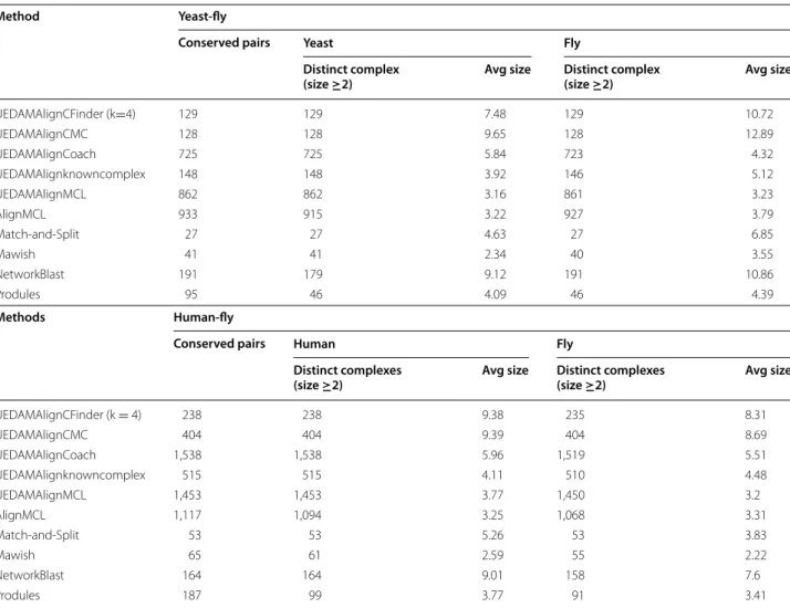
Table 1 shows the basic information of results of dif-ferent methods based on our experimental dataset. Col-umn “conserved pairs” refers to the number of conserved protein complexes pairs generated from alignment of two different PPI network. Since there exists many-to-many mappings between proteins of different PPI net-works, the conserved protein complexes in one network may be repeat and match with different ones in the other network. Additionally, a conserved protein complexes in on network may include some repeat proteins which are mapped to different proteins in the other network. Col-umn “distinct complexes (size ≥2)” refers to the number conserved protein complexes in one PPI network after filtering out repeat proteins in one complex and repeat complexes as well as those that consist of only one pro-tein. For example, AlignMCL yields 933 pairs of con-served protein complexes when comparing yeast PPI network against to fly PPI network. 915 out of 933 con-served protein complexes in yeast PPI network and 927 out of 933 conserved protein complexes in fly PPI net-work are distinct , each of which includes at least two dis-tinct proteins.
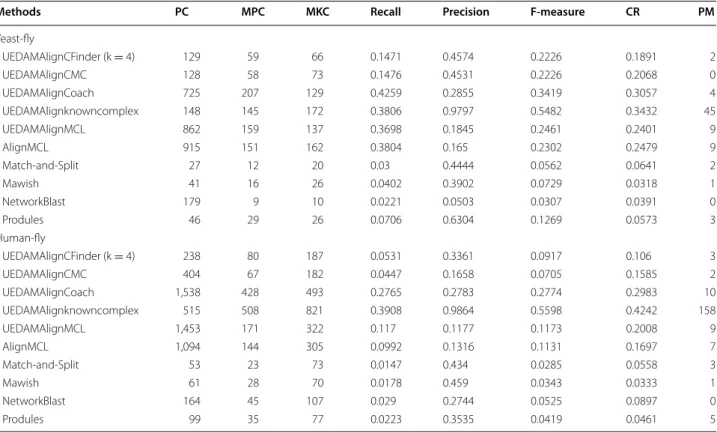
Table 2 shows the comparison of different methods by matching the predicted conserved protein complexes with known protein complexes. When using known com-plexes to partition PPI network, our method (UEDAMA-lignKnownComplex) detects 148 yeast conserved protein complexes (PC) and 515 human conserved protein com-plexes (PC), respectively when comparing yeast against fly and comparing human against fly. 145 out of 148 yeast conserved protein complexes match at least a known yeast complex (MPC), and 172 known yeast protein com-plexes match at least a predicted one (MKC). 508 out of 515 human conserved protein complexes match at least a known human complex (MPC), and 821 known human protein complexes match at least a predicted one (MKC). Moreover, UEDAMAlignKnownComplex detects 45 yeast and 158 human conserved protein complexes which share identical proteins with known yeast and human protein complexes, respectively (PM). The F-measure of UEDAMAlignKnownComplex is about 0.55 in align-ment of yeast and fly, and 0.56 in alignalign-ment of human and fly, which is the highest among all comparing meth-ods. When using computational methods to partition the PPI network, the performance of our methods varies due to their different performance of detecting protein com-plexes in a single PPI network. UEDAMAlignCoach pos-sesses the second best performance and its F-measure is 0.34 when aligning yeast with fly, which is 0.11, 0.28, 0.27, 0.29, 0.21 higher than AlignMCL, Match-and-Split, Mawish, NetworkBlast and Produles, respectively. When
aligning human with fly, the F-measure of UEDAMAlign-Coach achieves 0.28, which is 0.17, 0.25, 0.25, 0.23, 0.24 higher than AlignMCL, Match-and-Split, Mawish, Net-workBlast and Produles, respectively. As for coverage rate (CR), UEDAMAlignKnownComplex and UEDAMAlign-Coach also possess the first and the second best coverage rate in the two alignments. Here we don’t compare our methods with AlignNemo because AlignNemo cannot output results on our experimental dataset. AlignMCL takes the same strategy of constructing alignment graph as AlignNemo and are more scalable than AlignNemo, which has the best performance among other existing methods, including Match-and-Split, Mawish, Network-Blast and Produles, in term of F-measure and coverage rate. Both AlignMCL and UEDAMAlignMCL employ MCL method to partition PPI network. The difference is that the former uses MCL after constructing alignment graph while the latter uses it before aligning with the other PPI network. On the whole, UEDAMAlignMCL is
litter advanced than AlignMCL because its F-measure is litter higher than that of AlignMCL in two alignments. The CR value of DAMAlignMCL is higher than that of AlignMCL when comparing human against fly, while is almost the same as that of AlignMCL when comparing yeast against fly.
Biological relevance of conserved protein complex pairs
To further validate our method, we investigate biological relevance between the conserved protein complexes from the two different PPI networks, which is measured by the average of functional similarity among all proteins in them. Functional similarity of two proteins refers to the semantic similarity of their GO annotations [45]. Given two protein p1 and p2, and their GO annotations GO(p1) and GO(p2), the functional similarity between protein p1 and p2 is defined as follows:
(9) sim(p1,p2)=max(Resinksim(goi,goj))
Table 1 The basic information of results of different methods
Method Yeast-fly
Conserved pairs Yeast Fly
Distinct complex
(size ≥2) Avg size Distinct complex (size ≥2) Avg size
UEDAMAlignCFinder (k=4) 129 129 7.48 129 10.72 UEDAMAlignCMC 128 128 9.65 128 12.89 UEDAMAlignCoach 725 725 5.84 723 4.32 UEDAMAlignknowncomplex 148 148 3.92 146 5.12 UEDAMAlignMCL 862 862 3.16 861 3.23 AlignMCL 933 915 3.22 927 3.79 Match-and-Split 27 27 4.63 27 6.85 Mawish 41 41 2.34 40 3.55 NetworkBlast 191 179 9.12 191 10.86 Produles 95 46 4.09 46 4.39 Methods Human-fly
Conserved pairs Human Fly
Distinct complexes
(size ≥2) Avg size Distinct complexes (size ≥2) Avg size
UEDAMAlignCFinder (k = 4) 238 238 9.38 235 8.31 UEDAMAlignCMC 404 404 9.39 404 8.69 UEDAMAlignCoach 1,538 1,538 5.96 1,519 5.51 UEDAMAlignknowncomplex 515 515 4.11 510 4.48 UEDAMAlignMCL 1,453 1,453 3.77 1,450 3.2 AlignMCL 1,117 1,094 3.25 1,068 3.31 Match-and-Split 53 53 5.26 53 3.83 Mawish 65 61 2.59 55 2.22 NetworkBlast 164 164 9.01 158 7.6 Produles 187 99 3.77 91 3.41
where goi∈ GO(p1) and goj∈ GO(p2). Resinksim(goi, goj)
refers to the semantic similarity score of GO pair (goi, goj)
measured by Resink method [46]. In this work, we use Resinksim to measure the similarity between GO terms because both AlignNemo [17] and AlignMCL [21] use it. Based on Resink method, a free tool FastSemSim (http:// sourceforge.net/projects/fastsemsim/) is adopted to cal-culate the similarity of two proteins. The GO system con-sists of three separate categories of annotations, namely Molecular Function (MF), Biological Process (BP) and Cellular Component (CC). In this work, we mainly focus on the biological process (BP).
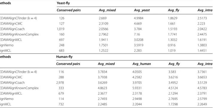
Table 3 shows the comparison of each method in terms of the functional similarity of conserved protein complex pairs, when comparing yeast against fly and comparing human against fly. Column “avg_yeast” and “avg_fly” refer to the average functional similarity of conserved yeast protein complexes and conserved fly protein complexes respectively when comparing yeast against fly. Column “avg_intra” lists the average func-tional similarity of conserved protein complex pair, when only considering the functional similarity between proteins from different species. Column “avg_mixed” lists the average functional similarity of conserved protein complex pair, when considering the functional similarity among all proteins, both inter-species and
intra-species. Results for two alignments show that UEDAMAlignKnownComplex yields conserved pro-tein complex pairs which are highly functional related, due to the highest avg_mixed values. Our method using computational methods, such as Coach, CMC and CFinder, to partition PPI networks, can also produce conserved protein complex pairs with similar functions, because their avg_mixed values for two alignments are higher than that of AlignMCL and NetworkBlast, com-parable to that of Produles and litter lower than that of Match-and-Split and Mawish. As for UEDAMAlign-MCL, it has relative lower avg_mixed values. However, its avg_mixed value is higher than that of AlignMCL for the alignment between yeast and fly, and comparable to that of AlignMCL for the alignment between human and fly.
Above results show that although previous methods such as Mawish, Produles and Match-and-Split can yield a small amount of conserved protein complexes that both match well with known protein complexes and are highly functional related, UEDAMAlign is able to detect more high quality conserved protein complexes that are func-tional related, if taking effective strategy to partition PPI network, i.e. inputting known protein complexes or those predicted by effective computational methods, such as Coach.
Table 2 Comparison of different methods in terms of how well matching with known proteins
Methods PC MPC MKC Recall Precision F-measure CR PM
Yeast-fly UEDAMAlignCFinder (k = 4) 129 59 66 0.1471 0.4574 0.2226 0.1891 2 UEDAMAlignCMC 128 58 73 0.1476 0.4531 0.2226 0.2068 0 UEDAMAlignCoach 725 207 129 0.4259 0.2855 0.3419 0.3057 4 UEDAMAlignknowncomplex 148 145 172 0.3806 0.9797 0.5482 0.3432 45 UEDAMAlignMCL 862 159 137 0.3698 0.1845 0.2461 0.2401 9 AlignMCL 915 151 162 0.3804 0.165 0.2302 0.2479 9 Match-and-Split 27 12 20 0.03 0.4444 0.0562 0.0641 2 Mawish 41 16 26 0.0402 0.3902 0.0729 0.0318 1 NetworkBlast 179 9 10 0.0221 0.0503 0.0307 0.0391 0 Produles 46 29 26 0.0706 0.6304 0.1269 0.0573 3 Human-fly UEDAMAlignCFinder (k = 4) 238 80 187 0.0531 0.3361 0.0917 0.106 3 UEDAMAlignCMC 404 67 182 0.0447 0.1658 0.0705 0.1585 2 UEDAMAlignCoach 1,538 428 493 0.2765 0.2783 0.2774 0.2983 10 UEDAMAlignknowncomplex 515 508 821 0.3908 0.9864 0.5598 0.4242 158 UEDAMAlignMCL 1,453 171 322 0.117 0.1177 0.1173 0.2008 9 AlignMCL 1,094 144 305 0.0992 0.1316 0.1131 0.1697 7 Match-and-Split 53 23 73 0.0147 0.434 0.0285 0.0558 3 Mawish 61 28 70 0.0178 0.459 0.0343 0.0333 1 NetworkBlast 164 45 107 0.029 0.2744 0.0525 0.0897 0 Produles 99 35 77 0.0223 0.3535 0.0419 0.0461 5
Validation based on experimental data of AlignNemo
Our UEDAMAlign method takes the same lenient cri-teria as AlignNemo does to align two PPI network. The main difference between the two methods lies in whether or not dividing PPI networks before aligning. However, AlignNemo cannot produce results when using our experimental data. For fair comparison, we compare our method with AlignNemo, as well as AlignMCL based on AlignNemo’s experimental data [17]. Table 4 shows the basic information of their results. The results of two alignment in Tables 5 and 6 show that UEDAMAlign-KnownComplex outperforms all comparing methods in term of its F-measure, coverage rate and Avg_mixed value, which suggest it can yield high quality conserved protein complexes not only matching well with known protein complexes but also highly functional related to their counterparts. UEDAMAlignCoach possesses the second best performance among all comparing methods in term of their F-measure and coverage rate. Its Avg_ mixed value is comparable to UEDAMAlignCFinder (k = 4), UEDAMAlignCMC. As for UEDAMAlignCFinder and AignNemo, UEDAMAlignCFinder (k = 4) divides PPI network by using CFinder to detect the 4-cliques in
a PPI network, and AignNemo detects conserved protein complexes from alignment graph by extracting 4-sub-graphs. DAMAlignCFinder (k = 4) has higher F-measure and Avg_mixed value than AignNemo and comparable coverage rate to AlignNemo. As for DAMAlignMCL and AlignMCL, both methods use MCL method to partition network before or after aligning two network. UEDA-MAlignMCL has higher F-measure and Avg_mixed value than AignMCL and comparable coverage rate to Align-MCL. All of these facts verify the effectiveness of our methods that take the dividing-and-matching strategy to align two networks.
Effect of parameters on performance
The other contribution of UEDAMAlign lies in being capable of taking unequally lenient criteria when com-paring two PPI networks. It makes use of two param-eters l and r to control the walking steps taken in the two input PPI networks and therefore determine the distance that a protein pair can span in corresponding network. For example, when aligning the network of yeast and fruit fly, setting parameter l and r to 2 and 3 respectively means that UEDAMAlign locally extends a Table 3 Comparison in terms of biological relevance between each pair of conserved protein complexes predicted by each method
Methods Yeast-fly
Conserved pairs Avg_mixed Avg_yeast Avg_fly Avg_intra
UEDAMAlignCFinder (k = 4) 129 3.96 5.3766 3.4259 3.7503 UEDAMAlignCMC 128 3.5266 4.9468 2.9469 3.3061 UEDAMAlignCoach 725 3.4729 4.4809 2.5707 3.1565 UEDAMAlignKnownComplex 148 4.5041 7.0767 3.7421 3.9779 UEDAMAlignMCL 862 2.3539 3.2412 1.4475 2.3063 AlignMCL 933 2.2563 2.9469 1.255 2.2319 Match-and-Split 27 4.069 5.7868 3.3512 3.614 Mawish 41 4.4942 5.9584 3.7828 4.2566 NetworkBlast 191 2.2865 2.8698 1.8388 2.198 Produles 95 3.4301 6.3427 2.525 2.8541 Methods Human-fly
Conserved pairs Avg_mixed Avg_human Avg_fly Avg_intra
UEDAMAlignCFinder (k = 4) 238 3.7826 4.0948 3.7551 3.6892 UEDAMAlignCMC 404 3.5078 4.0341 3.2929 3.3612 UEDAMAlignCoach 1,538 3.5807 4.0532 3.3599 3.4388 UEDAMAlignKnownComplex 515 4.8490 6.1202 4.4131 4.5720 UEDAMAlignMCL 1,453 2.2718 2.4197 1.905 2.2812 AlignMCL 1,117 2.4166 2.5095 1.7317 2.456 Match-and-Split 53 4.0713 4.484 4.6043 3.7865 Mawish 65 4.424 4.8343 4.9263 4.1549 NetworkBlast 164 3.3956 3.7568 3.3467 3.2386 Produles 187 3.8828 4.3098 4.2651 3.7342
pair of homologous proteins if there exists one path of length not larger than 2 to connect the yeast node in the homologous protein pair or one path of length not larger than 3 to connect the fruit fly node in the homol-ogous protein pair. Specially, as l and r are both set to
2, UEDAMAlign achieves the same performance to DAMAlign on detecting conserved protein complexes. To investigate the effect of unequally lenient strategy on the performance of detecting conserved protein com-plexes, we vary the two parameters ranging from 2 to 3 Table 4 The basic information of results of different methods based on AlingNemo’s dataset
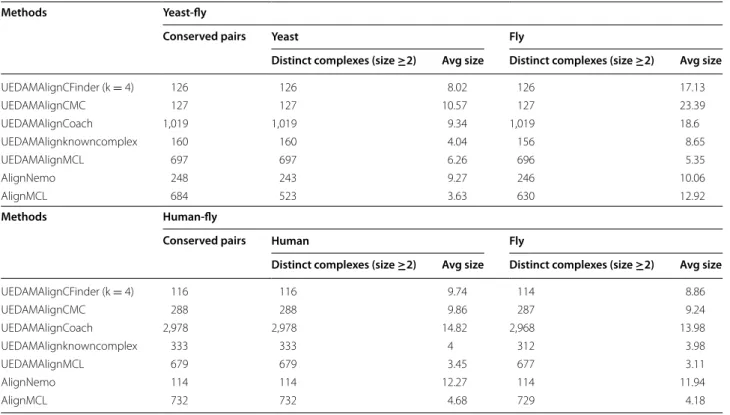
Methods Yeast-fly
Conserved pairs Yeast Fly
Distinct complexes (size ≥2) Avg size Distinct complexes (size ≥2) Avg size
UEDAMAlignCFinder (k = 4) 126 126 8.02 126 17.13 UEDAMAlignCMC 127 127 10.57 127 23.39 UEDAMAlignCoach 1,019 1,019 9.34 1,019 18.6 UEDAMAlignknowncomplex 160 160 4.04 156 8.65 UEDAMAlignMCL 697 697 6.26 696 5.35 AlignNemo 248 243 9.27 246 10.06 AlignMCL 684 523 3.63 630 12.92 Methods Human-fly
Conserved pairs Human Fly
Distinct complexes (size ≥2) Avg size Distinct complexes (size ≥2) Avg size
UEDAMAlignCFinder (k = 4) 116 116 9.74 114 8.86 UEDAMAlignCMC 288 288 9.86 287 9.24 UEDAMAlignCoach 2,978 2,978 14.82 2,968 13.98 UEDAMAlignknowncomplex 333 333 4 312 3.98 UEDAMAlignMCL 679 679 3.45 677 3.11 AlignNemo 114 114 12.27 114 11.94 AlignMCL 732 732 4.68 729 4.18
Table 5 Comparison of different methods in terms of how well matching with known protein based one AlignNemo’s dataset
Methods PC MPC MKC Recall Precision F-measure CR PM
Yeast-fly UEDAMAlignCFinder (k = 4) 126 62 66 0.1535 0.4921 0.234 0.1682 2 UEDAMAlignCMC 127 57 74 0.1458 0.4488 0.2201 0.2208 0 UEDAMAlignCoach 1,019 190 134 0.4095 0.1865 0.2562 0.288 0 UEDAMAlignknowncomplex 160 158 184 0.4136 0.9875 0.583 0.3745 47 UEDAMAlignMCL 697 113 115 0.2783 0.1621 0.2049 0.2365 4 AlignNemo 243 77 53 0.1782 0.3169 0.2281 0.1755 0 AlignMCL 523 95 97 0.234 0.1816 0.2045 0.2224 5 Human-fly UEDAMAlignCFinder (k = 4) 116 42 67 0.0264 0.3621 0.0493 0.0451 1 UEDAMAlignCMC 288 62 101 0.0394 0.2153 0.0666 0.1251 1 UEDAMAlignCoach 2,978 432 281 0.2449 0.1451 0.1822 0.1945 0 UEDAMAlignknowncomplex 333 326 552 0.235 0.979 0.3791 0.2634 34 UEDAMAlignMCL 679 103 219 0.0688 0.1517 0.0947 0.1459 2 AlignNemo 114 31 48 0.0194 0.2719 0.0363 0.0628 0 AlignMCL 732 97 254 0.0666 0.1325 0.0887 0.2012 2
and evaluate the prediction accuracy of UEDAMAlign when utilizing known protein complexes or Coach to partition the input PPI networks.
Tables 7 and 8 show that in the two alignments, UEDA-MAlign does not always possess the best performance
when its parameters l and r are both set to 2 in terms of F-measures values and Avg_mixed values. For example, as aligning human and fruit fly, UEDAMAlignKnown-Complex when the parameters l and r are set to 3 and 2 outperforms that when the parameters l and r are both Table 6 Comparison in terms of biological relevance between each pair of conserved protein complexes predicted by each method based one AlignNemo’s dataset
Methods Yeast-fly
Conserved pairs Avg_mixed Avg_yeast Avg_fly Avg_intra
UEDAMAlignCFinder (k = 4) 126 2.669 4.9984 1.8629 2.5173 UEDAMAlignCMC 127 2.3109 4.669 1.661 2.223 UEDAMAlignCoach 1,019 2.0566 3.784 1.5193 2.0422 UEDAMAlignKnownComplex 160 2.7962 7.16 1.7741 2.4475 UEDAMAlignMCL 697 1.9411 3.0208 1.3032 1.6191 AlignNemo 248 1.7501 3.5919 0.916 1.3803 AlignMCL 683 1.2522 2.283 1.019 1.4451 Methods Human-fly
Conserved pairs Avg_mixed Avg_human Avg_fly Avg_intra
UEDAMAlignCFinder (k = 4) 116 3.7834 4.0505 3.583 3.7361 UEDAMAlignCMC 288 3.7938 4.2582 3.6216 3.6653 UEDAMAlignCoach 2,978 3.6269 3.9705 3.4952 3.5129 UEDAMAlignKnownComplex 333 4.8623 5.9331 4.5124 4.5783 UEDAMAlignMCL 679 2.3677 2.3178 2.1294 2.3791 AlignNemo 114 2.7493 2.9498 2.7695 2.5799 AlignMCL 732 2.2485 2.2044 1.7298 2.2649
Table 7 Comparison of performance of UEDAMAlignKnownComplex and UEDAMAlignCoach with respect to various val-ues of parameter l and r on how well matching with known protein
Methods PC MPC MKC Recall Precision F-measure CR PM
Yeast-fly UEDAMAlignCoach_l=2_r=2 725 207 129 0.4259 0.2855 0.3419 0.3057 4 UEDAMAlignCoach_l=2_r=3 762 214 144 0.4477 0.2808 0.3452 0.3078 4 UEDAMAlignCoach_l=3_r=2 785 217 142 0.4493 0.2764 0.3423 0.3078 4 UEDAMAlignCoach_l=3_r=3 785 218 144 0.4523 0.2777 0.3441 0.3078 4 UEDAMAlignKnowComplex_l=2_r=2 148 145 172 0.3806 0.9797 0.5482 0.3432 45 UEDAMAlignKnowComplex_l=2_r=3 149 146 173 0.3832 0.9799 0.5509 0.3453 46 UEDAMAlignKnowComplex_l=3_r=2 148 145 172 0.3806 0.9797 0.5482 0.3432 45 UEDAMAlignKnowComplex_l=3_r=3 149 146 173 0.3832 0.9799 0.5509 0.3453 46 Human-fly UEDAMAlignCoach_l=2_r=2 1,538 428 493 0.2765 0.2783 0.2774 0.2983 10 UEDAMAlignCoach_l=2_r=3 1,420 410 474 0.2647 0.2887 0.2762 0.2963 9 UEDAMAlignCoach_l=3_r=2 1,421 401 469 0.2595 0.2822 0.2704 0.2965 9 UEDAMAlignCoach_l=3_r=3 1,430 406 473 0.2626 0.2839 0.2728 0.2965 9 UEDAMAlignKnowComplex_l=2_r=2 515 508 821 0.3908 0.9864 0.5598 0.4242 158 UEDAMAlignKnowComplex_l=2_r=3 521 514 826 0.3951 0.9866 0.5642 0.4269 158 UEDAMAlignKnowComplex_l=3_r=2 522 515 827 0.3958 0.9866 0.5650 0.4270 158 UEDAMAlignKnowComplex_l=3_r=3 524 517 829 0.3974 0.9866 0.5666 0.4274 158
set to 2. It means that taking unequally lenient crite-ria on the two input networks by setting suitable val-ues to the parameters can improve the performance of UEDAMAlign.
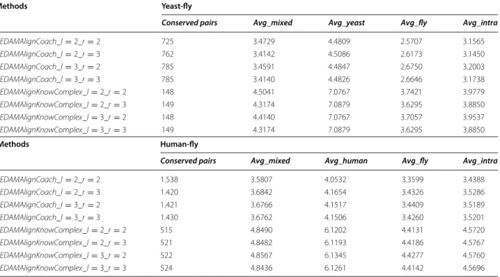
As Table 7 shown, no matter which one of the two partition methods UEDAMAlign uses, for the align-ment of yeast and fruit fly, its highest F-measure val-ues achieve when setting the parameters l and r to unequal values. Specially, both UEDAMAlignKnown-Complex and UEDAMAlignCoach achieve the highest F-measures as the parameters l and r are set to 2 and 3. For the alignment of human and fruit fly, UEDAMA-lign has the highest F-measure values when setting the parameters l and r to equal values. Specially, UEDA-MAlignKnownComplex has the highest F-measures value as the two parameters are set to 2 and UEDA-MAlignCoach achieves the highest F-measures value as setting the two parameter to 3. Through analyzing the structure and topology of the three PPI networks, we find that the yeast PPI network contains 5,093 proteins and 22,570 interactions, whose average path length is about 3.84, the fruit fly PPI network con-tains 7,916 GO terms and 20,289 edges, whose average path length is about 4.5, while the human PPI net-work includes 13,398 proteins and 86,307 interactions, whose average path length is about 4.2. It is obvious
that the PPI network of fruit fly is sparser than that of yeast and is similar dense to that of human, which may cause the difference in criteria for comparing the two pairs of PPI networks.
Table 8 show that the conserved protein complexes that can well match with known protein complexes are less biological relevant.
For example, as the parameters l and r are set to 2 and 3, UEDAMAlignKnownComplex and UEDAMA-lignCoach achieve the highest F-measures when align-ing yeast and fruit fly. However, the conserved protein complexes detected by them under this condition have lower biological relevance duo to the lowest Avg_mixed values. This may be caused by two reasons. The one may be homologous protein pairs with low functional similarity are introduced to identified conserved pro-tein complexes. The other is the propro-teins in conserved protein complexes have some similar functions with their homologous proteins, which are not found by biologist.
The results in Tables 7 and 8 verify that UEDAMAlign can taking unequally lenient criteria on the two compar-ing PPI network by settcompar-ing parameters l and r. However, it is still a big challenge for us to choose suitable values for parameters l and r with respect to the difference between the two input networks.
Table 8 Comparison in terms of biological relevance between each pair of conserved protein complexes predicted by UEDAMAlignKnownComplex and UEDAMAlignCoach with respect to various values of parameter l and r
Methods Yeast-fly
Conserved pairs Avg_mixed Avg_yeast Avg_fly Avg_intra
UEDAMAlignCoach_l=2_r=2 725 3.4729 4.4809 2.5707 3.1565 UEDAMAlignCoach_l=2_r=3 762 3.4142 4.5086 2.6173 3.1450 UEDAMAlignCoach_l=3_r=2 785 3.4591 4.4847 2.6750 3.2003 UEDAMAlignCoach_l=3_r=3 785 3.4140 4.4826 2.6646 3.1738 UEDAMAlignKnowComplex_l=2_r=2 148 4.5041 7.0767 3.7421 3.9779 UEDAMAlignKnowComplex_l=2_r=3 149 4.3174 7.0879 3.6295 3.8850 UEDAMAlignKnowComplex_l=3_r=2 148 4.4140 7.0767 3.7057 3.9537 UEDAMAlignKnowComplex_l=3_r=3 149 4.3174 7.0879 3.6295 3.8850 Methods Human-fly
Conserved pairs Avg_mixed Avg_human Avg_fly Avg_intra
UEDAMAlignCoach_l=2_r=2 1.538 3.5807 4.0532 3.3599 3.4388 UEDAMAlignCoach_l=2_r=3 1.420 3.6842 4.1654 3.4326 3.5286 UEDAMAlignCoach_l=3_r=2 1.421 3.6766 4.1517 3.4409 3.5189 UEDAMAlignCoach_l=3_r=3 1.430 3.6762 4.1506 3.4260 3.5201 UEDAMAlignKnowComplex_l=2_r=2 515 4.8490 6.1202 4.4131 4.5720 UEDAMAlignKnowComplex_l=2_r=3 521 4.8482 6.1193 4.4186 4.5767 UEDAMAlignKnowComplex_l=3_r=2 522 4.8567 6.1345 4.4277 4.5760 UEDAMAlignKnowComplex_l=3_r=3 524 4.8436 6.1261 4.4142 4.5696
Conclusion
The aim of this work is to detect protein complexes con-served across species through locally aligning a pair of PPI networks. Most of previous methods adopt equally lenient criteria on the two comparing networks but fail to consider the differences of the two networks. Consid-ering that PPI network has the property of modularity and increasing number of known protein complex data are available, we propose a new dividing-and-match-ing-based method named by UEDAMAlign to detect conserved protein complexes. UEDAMAlign detects subnetworks from one of PPI network and maps these subnetworks to the other one. After that, UEDAMAlign takes heuristic strategy to find the common connected components from the subnetworks and their homolo-gous proteins in the other network. In the course of find-ing common connected components, UEDAMAlign takes lenient criteria which may vary with parameters according to topological feature of input PPI networks. To access the effectiveness of UEDAMAlign. we carry out two alignments, yeast with fruit fly, and human with fruit fly. Comparison are made between other existing meth-ods and UEDAMAlign when taking the same lenient cri-teria as AlignNemo and DAMAlign to extend locally a pair of homologous proteins (parameters l and r are set to 2). (1) The experimental results shows that UEDAMAlign is superior to all other methods in recovering conserved protein complexes which can both match known pro-tein complexes well and have similar functions if it takes effective strategies to partition PPI networks, for exam-ple using known protein comexam-plexes or Coach to parti-tion. (2) UEDAMAlignMCL outperforming AlignMCL and UEDAMAlignCFinder outperforming AlignNemo confirm the effectiveness of dividing-and-matching strat-egy of our UEDAMAlign method. (3) The experimental results when setting various values for the parameters (l and r) of UEDAMAlign verify that UEDAMAlign can taking unequally lenient criteria on the two comparing PPI network by setting parameters l and r. However, it is still a big challenge for us to choose suitable values for parameters l and r with respect to the difference between the two input networks.
Author’s contributions
WP obtained the protein–protein interaction data, protein sequence data and protein complex data. JXW, WP and FxW designed the new methods and analyzed the results. WP and Jxw drafted the manuscript together. FXW participated in revising the draft. All authors read and approved the final manuscript.
Author details
1 The School of Information Science and Engineering, Central South University, Changsha, Hunan, People’s Republic of China. 2 The Faculty of Information Engineering and Automation, Kunming University of Science and Technology, Kunming 650093, Yunnan, People’s Republic of China. 3 Division of Biomedical
Engineering, Department of Mechanical Engineering, University of Saskatch-ewan, Saskatoon, SK S7N 5A9, Canada. 4 Department of Computer Science, Georgia State University, Atlanta, GA 30302-4110, USA.
Acknowledgements
This work is supported in part by the National Natural Science Foundation of China under Grant No. 61232001, No. 61379108 and No. 61370024. Declarations
The publication costs for this article were funded by the corresponding author.
Compliance with ethical guidelines Competing interests
The authors declare that they have no competing interests. Received: 30 September 2014 Accepted: 26 May 2015
References
1. Wuchty S, Oltvai ZN, Barabási A-L (2003) Evolutionary conservation of motif constituents in the yeast protein interaction network. Nat Genet 35(2):176–179
2. Li X, Wu M, Kwoh C-K, Ng S-K (2010) Computational approaches for detecting protein complexes from protein interaction networks: a survey. BMC Genomic 11(Suppl 1):3
3. Li M, Wang J, Chen J, Cai Z (2010) Identifying the overlapping complexes in protein interaction networks. Int J Data Min Bioinform 4(1):91–108 4. Li M, Wu X, Wang J, Pan Y (2012) Towards the identification of protein
complexes and functional modules by integrating PPI network and gene expression data. BMC Bioinform 13(1):109
5. Tang X, Wang J, Liu B, Li M, Chen G, Pan Y (2011) A comparison of the functional modules identified from time course and static PPI network data. BMC Bioinform 12(1):339
6. Peng W, Wang J, Zhao B, Wang L (2014) Identification of protein complexes using weighted pagerank-nibble algorithm and core-attach-ment structure. IEEE/ACM Trans Comput Biol Bioinform. doi:10.1109/ TCBB.2014.2343954
7. Tang X, Wang J, Li M, He Y, Pan Y (2014) A novel algorithm for detecting protein complexes with the breadth first search. BioMed Res Int 2014:1–8 Art. ID 354539. doi:10.1155/2014/354539
8. Li M, Chen W, Wang J, Wu F-X, Pan Y (2014) Identifying dynamic protein complexes based on gene expression profiles and PPI networks. BioMed Res Int 2014:1–10 Art. ID 375262. doi:10.1155/2014/375262
9. Wang J, Zhong J, Chen G, Li M, Wu F-X, Pan Y (2014) Clusterviz: a cytoscape app for clustering analysis of biological network. IEEE/ACM Trans Comput Biol Bioinform. doi:10.1109/TCBB.2014.2361348
10. Sharan R, Ideker T (2006) Modeling cellular machinery through biological network comparison. Nat Biotechnol 24(4):427–433
11. Singh R, Xu J, Berger B (2007) Pairwise global alignment of protein inter-action networks by matching neighborhood topology. Res Comput Mol Biol 4453:16–31
12. Atias N, Sharan R (2013) ipoint: an integer programming based algorithm for inferring protein subnetworks. Mol BioSyst 9(7):1662–1669
13. Yosef N, Kupiec M, Ruppin E, Sharan R (2009) A complex-centric view of protein network evolution. Nucleic Acids Res 37(12):88–88
14. Nguyen P-V, Srihari S, Leong HW (2013) Identifying conserved protein complexes between species by constructing interolog networks. BMC Bioinform 14(16):1–16
15. Vanunu O, Magger O, Ruppin E, Shlomi T, Sharan R (2010) Associating genes and protein complexes with disease via network propagation. PLoS Comput Biol 6(1):1000641
16. Ali W, Deane CM (2009) Functionally guided alignment of protein interac-tion networks for module detecinterac-tion. Bioinformatics 25(23):3166–3173 17. Ciriello G, Mina M, Guzzi PH, Cannataro M, Guerra C (2012) Alignnemo: a
local network alignment method to integrate homology and topology. PLoS One 7(6):38107
18. Sharan R, Ideker T, Kelley B, Shamir R, Karp RM (2005) Identification of protein complexes by comparative analysis of yeast and bacterial protein interaction data. J Comput Biol 12(6):835–846
19. Koyutürk M, Kim Y, Topkara U, Subramaniam S, Szpankowski W, Grama A (2006) Pairwise alignment of protein interaction networks. J Comput Biol 13(2):182–199
20. Cootes AP, Muggleton SH, Sternberg MJ (2007) The identification of similarities between biological networks: application to the metabolome and interactome. J Mol Biol 369(4):1126–1139
21. Mina M, Guzzi P (2014) Improving the robustness of local network align-ment: design and extensive assessment of a markov clustering-based approach. IEEE/ACM Trans Comput Biol Bioinform 11(3):561–572 22. Jancura P, Marchiori E (2010) Dividing protein interaction networks
for modular network comparative analysis. Pattern Recogn Lett 31(14):2083–2096
23. Li Z, Zhang S, Wang Y, Zhang X-S, Chen L (2007) Alignment of molecu-lar networks by integer quadratic programming. Bioinformatics 23(13):1631–1639
24. Hodgkinson L, Karp RM (2012) Algorithms to detect multiprotein modu-larity conserved during evolution. IEEE/ACM Trans Comput Biol Bioinform (TCBB) 9(4):1046–1058
25. Peng W, Wang J, Wu F (2013) A dividing-and-matching algorithm to detect conserved protein complexes via local network alignment. In: 2013 IEEE international bioinformatics and biomedicine conference (BIBM) on 18–21 Dec. 2013, pp 78–81 (2013)
26. Wang J, Li M, Chen J, Pan Y (2011) A fast hierarchical clustering algorithm for functional modules discovery in protein interaction networks. IEEE/ ACM Trans Comput Biol Bioinform 8(3):607–620
27. Zhao B, Wang J, Li M, Wu F, Pan Y (2014) Detecting protein complexes based on uncertain graph model. IEEE/ACM Trans Comput Biol Bioinform. doi:10.1109/TCBB.2013.2297915
28. Wang J, Peng X, Peng W, Wu F-X (2014) Dynamic protein interaction network construction and applications. Proteomics 14(4–5):338–352 29. Wang J, Peng X, Li M, Pan Y (2013) Construction and application of
dynamic protein interaction network based on time course gene expres-sion data. Proteomics 13(2):301–312
30. Wang J, Peng X, Xiao Q, Li M, Pan Y (2013) An effective method for refining predicted protein complexes based on protein activity and the mechanism of protein complex formation. BMC Syst Biol 7(1):28 31. Kelley BP, Sharan R, Karp RM, Sittler T, Root DE, Stockwell BR et al (2003)
Conserved pathways within bacteria and yeast as revealed by global protein network alignment. Proc Natl Acad Sci 100(20):11394–11399
32. Pache RA, Céol A, Aloy P (2012) Netaligner-a network alignment server to compare complexes, pathways and whole interactomes. Nucleic Acids Res 40(W1):157–161
33. Narayanan M, Karp RM (2007) Comparing protein interaction networks via a graph match-and-split algorithm. J Comput Biol 14(7):892–907 34. Andersen R, Chung F, Lang K (2007) Using pagerank to locally partition a
graph. Internet Math 4(1):35–64
35. Peng W, Wang J, Chen L, Zhong J, Zhang Z, Pan Y (2014) Predicting protein functions by using unbalanced bi-random walk algorithm on protein–protein interaction network and functional interrelationship network. Curr Protein Pept Sci 15(6):529–539
36. Wu M, Li X, Kwoh C-K, Ng S-K (2009) A core-attachment based method to detect protein complexes in PPI networks. BMC Bioinform 10(1):169 37. van Dongen SM (2000) Graph clustering by flow simulation. Ph.D. thesis,
University of Utrecht, The Netherlands
38. Enright AJ, Van Dongen S, Ouzounis CA (2002) An efficient algo-rithm for large-scale detection of protein families. Nucleic Acids Res 30(7):1575–1584
39. Liu G, Wong L, Chua HN (2009) Complex discovery from weighted PPI networks. Bioinformatics 25(15):1891–1897
40. Adamcsek B, Palla G, Farkas IJ, Derényi I, Vicsek T (2006) Cfinder: locating cliques and overlapping modules in biological networks. Bioinformatics 22(8):1021–1023
41. Xenarios I, Salwinski L, Duan XJ, Higney P, Kim S-M, Eisenberg D (2002) Dip, the database of interacting proteins: a research tool for studying cellular networks of protein interactions. Nucleic Acids Res 30(1):303–305 42. Schaefer MH, Fontaine J-F, Vinayagam A, Porras P, Wanker EE,
Andrade-Navarro MA (2012) Hippie: integrating protein interaction networks with experiment based quality scores. PLoS One 7(2):31826
43. Pu S, Wong J, Turner B, Cho E, Wodak SJ (2009) Up-to-date catalogues of yeast protein complexes. Nucleic Acids Res 37(3):825–831
44. Ruepp A, Waegele B, Lechner M, Brauner B, Dunger-Kaltenbach I, Fobo G et al (2010) Corum: the comprehensive resource of mammalian protein complexes. Nucleic Acids Res 38(suppl 1):497–501
45. Guzzi PH, Mina M, Guerra C, Cannataro M (2012) Semantic similarity analysis of protein data: assessment with biological features and issues. Brief Bioinform 13(5):569–585
46. Resnik P (1999) Semantic similarity in a taxonomy: an information-based measure and its application to problems of ambiguity in natural lan-guage. J Artif Intell Res 11:95–130
Submit your next manuscript to BioMed Central and take full advantage of:
• Convenient online submission • Thorough peer review
• No space constraints or color figure charges • Immediate publication on acceptance
• Inclusion in PubMed, CAS, Scopus and Google Scholar • Research which is freely available for redistribution Submit your manuscript at