Development of a framework to compare the cost-effectiveness of traffic crash countermeasures

(1)

2017

Development of a framework to compare the

cost-effectiveness of traffic crash countermeasures

Patricia Anne Thompson

Iowa State University

Follow this and additional works at:https://lib.dr.iastate.edu/etd

Part of theCivil Engineering Commons, and theTransportation Commons

This Thesis is brought to you for free and open access by the Iowa State University Capstones, Theses and Dissertations at Iowa State University Digital Repository. It has been accepted for inclusion in Graduate Theses and Dissertations by an authorized administrator of Iowa State University Digital Repository. For more information, please [email protected].

Recommended Citation

Thompson, Patricia Anne, "Development of a framework to compare the cost-effectiveness of traffic crash countermeasures" (2017).

Graduate Theses and Dissertations. 15437. https://lib.dr.iastate.edu/etd/15437

(2)

Development of a framework to compare the cost-effectiveness of traffic crash countermeasures

by

Patricia Thompson

A thesis submitted to the graduate faculty

in partial fulfillment of the requirements for the degree of MASTER OF SCIENCE

Major: Civil Engineering (Transportation Engineering)

Program of Study Committee: Peter Savolainen, Major Professor

Shauna Hallmark Peng Wei

The student author and program of study committee are solely responsible for the content of this thesis. The Graduate College will ensure this thesis is globally accessible and will not

permit alterations after a degree is conferred.

Iowa State University Ames, Iowa

2017

(3)

As the transportation industry moves towards an ultimate goal of zero deaths on roads in the United States, decisions are made every day regarding how to best utilize limited transportation funding for the implementation of crash countermeasures. At a time when many jurisdictions face difficulties in maintaining their existing infrastructure, additional tools are necessary to ensure that available funding is spent in the most productive manner. Determining whether or not a crash countermeasure is financially justified is one of the primary considerations in transportation agencies’ planning and programming efforts. However, a myriad of analytical concerns limit the ability to effectively determine the cost-effectiveness of specific countermeasures. Using a series of locally-derived safety

performance functions (SPFs) and severity distribution functions (SDFs), this study provides a set of tools that can be used to assess the feasibility of potential countermeasures for various location types (e.g., segments, intersections, etc.). Construction cost data for a series of countermeasures can be integrated with robust crash modification factors (CMFs),

allowing for a flexible economic analysis framework in which competing or complementary countermeasures can be evaluated. The final product of this project provides decision-makers with a planning-level tool that will allow for direct consideration of the prospective economic impacts and related uncertainty that is inherent in such estimates.

(12)

CHAPTER 1: INTRODUCTION 1.1Background

Every year in the United States, more than 30,000 people are killed due to roadway related crashes (FARS, 2016). The total number of fatalities can fluctuate widely from year to year but, as illustrated in Figure 1, general trends show that traffic fatalities have been declining over the last 35 years. To control for variations in exposure (e.g., fluctuations in the miles traveled each year), it is better to look at the rate of fatalities per 100 million vehicle miles traveled (VMT), which have been decreasing steadily, excluding a small increase around 1985, until 2010. Over the time period shown in Figure 1, the fatality rate started at a high of 3.35 fatalities per 100 million VMT in 1980 and decreased to approximately 1.5 fatalities per 100 million VMT in 2005. At this point, as part of their Strategic Highway Safety Plan, the American Association of State Highway and Transportation Officials

(AASHTO) set a goal to lower the fatality rate to 1.0 fatalities per 100 million VMT by 2008 (AASHTO, 2005). This goal was close to being realized by 2010, but few further

improvements have been made; the fatality rate has fluctuated around the 1.1 fatalities per 100 million VMT since 2010.

(13)

Figure 1. Traffic Related Fatalities in the US, 1980 to 2015, by Total and Rate

The decline can be attributed to several factors. Vehicle safety has improved dramatically over the years. For example, the invention of anti-lock brakes has allowed drivers to maintain better control of their vehicles when the brakes would have otherwise locked up and not allowed for steering to occur (Burton, 2004). In a 2012 study, it was determined that there was a 5 percent decrease in crash probability and a 3 percent increase in the probability of being uninjured if a crash did occur in a 2008 vehicle vs a 2000 vehicle (Glassbrenner 2012). Efforts have been also made to address unsafe driving behaviors. Public awareness campaigns about issues such as seat belt use and child restraints have had a

positive impact on citizen compliance with the laws. Usage of a seat belt can reduce the risk of death for a front-seat occupant by 45 to 60 percent (NHTSA). Increased seat belt use in the US, particularly since the institution of the Click It or Ticket campaign, implemented in all states in 2004, can therefore be partially linked to a decrease in fatalities. Safety

1 1.5 2 2.5 3 3.5 30000 35000 40000 45000 50000 55000 1980 1985 1990 1995 2000 2005 2010 2015

Fatalities per

100 million

VMT

T

o

tal Fatalities

Year

(14)

countermeasures are also likely responsible for some of the decrease in fatalities. Cable median barrier has been shown to reduce the number of cross-median head-on fatal crashes by nearly 50 percent (Olson et al. 2013). The addition of a crash cushion at a roadside fixed object can reduce fatal and injury crashes by 69 percent (Elvik and Vaa, 2004). Turning a 4 lane undivided roadway into a 3 lane roadway with a two-way left-turn lane can reduce crashes by 15 to 25 percent (Pawlovich et al. 2006). Other safety treatments have had similar, if less drastic, results.

The way transportation agencies have evaluated traffic safety has likewise changed in recent years, including the ways in which road facilities have been classified in terms of their safety or risk potential. For many years, a roadway was considered “nominally” safe if it met all the relevant minimum design criteria in design manuals, such as AASHTO’s A Policy on Geometric Design of Highways and Streets (also known as the “Green Book”) (AASHTO, 2011). For example, so long as the minimum turning radius was sufficient for the functional class, the street was considered safe.

This way of approaching safety largely changed in 2010 with the introduction of the AASHTO Highway Safety Manual (HSM) (AASHTO 2010). Instead of focusing on nominal safety, the HSM outlines a variety of state-of-the-art methods to determine if a roadway is substantively, or quantitatively, safe through the use of data analytics. Crash rates and frequencies are compared across similar types of locations using various methods to

determine if statistically significant differences exist and whether specific locations present higher risk. These methods include: before-and-after studies, which compare the

(15)

cross-sectional studies, where similar locations are compared, some of which have the treatment while others do not; and combinations of these and others.

Safety performance functions (SPFs) and severity distribution functions (SDFs) are important facets of traffic safety data analysis using the methods outlined in the HSM. Due to the fact that crash countermeasures are rarely implemented on a system-wide basis due to budget constraints, sites tend to be selected based on the basis of disproportionately high crash frequencies or rates (calculated using the appropriate exposure variable, annual average daily traffic (AADT), VMT, or daily entering vehicles (DEV)). Given that crashes tend to be rare and random, a decrease in crashes at a specific location may simply be due to normal fluctuation, potentially leading to an overestimation of the effectiveness of a specific countermeasure. One method of addressing this regression-to-the-mean (RTM) bias is to calculate the expected number of crashes for that site. The most widely applied method for addressing RTM is known as the empirical Bayes (EB) method and is outlined in the HSM. The EB framework combines the long-term crash history at a given location with the

predicted number of crashes as determined by a regression model developed using data from sites that are similar to where the treatment has been applied. SPFs and SDFs are generally used to calculate the predicted number of crashes.

The influence of analytics can also be seen when deciding what projects to fund. Cost effectiveness evaluation is a way of determining if the total benefit from the project is equal to the cost of implementing it. When dealing with limited funds for projects, it is important that the most cost effective solutions are selected, that is, the solutions that provide more benefits than costs. In terms of traffic safety countermeasures, if the total value of the crashes

(16)

prevented, translated into dollars, does not exceed the total cost of implementing the countermeasure, it is very likely that the money could better spent elsewhere.

One practical limitation of the HSM is that the processes and underlying statistical methods on which they are derived can be very complex. For even experienced practitioners, the safety planning process can be very time- and resource-intensive. Beginning with

calibrating the HSM provided SPFs with local crash data, the practitioner must have historical data available from the roadways in the jurisdiction over time. If the SPFs have already been calibrated, then the practitioner must use the various SPFs (fatal/injury (FI) single vehicle, fatal/injury multi-vehicle non-driveway, property damage only (PDO) single vehicle, PDO multi-vehicle non-driveway) to calculate predicted crashes and then use an SDF to estimate how many crashes of each type would occur at each injury severity level.

Next, for project feasibility studies, the economic costs of those crashes over time must be forecasted and the present (or annual) value calculated. The installation and maintenance costs of the countermeasure must also be estimated for the service life of the countermeasure. Then, these crash cost savings and agency cost values may be used to calculate the benefit cost ratio or various other metrics. Therefore, determining a single number for one site can require a substantial investment in terms of time and data, making it particularly difficult when attempting to compare several projects across different candidate sites to determine the most cost-effective alternatives.

1.2Research Objectives

The objective of this thesis was to develop an easy-to-use analysis tool to allow transportation professionals and decision makers to assess the economic feasibility of

(17)

for its application across different jurisdictions. This is important as research suggests safety performance and the related predictive equations tend to vary across geographic areas due to unobserved factors beyond traffic characteristics and crash rates, necessitating calibration of generalized models, estimation of new ones, or other methods to account for local conditions (Chen 2012). The tool integrates a series of SPFs, which account for the effects of AADT and regional effects to predict the number of crashes occurring on urban and suburban road segments. The tool is presented using data drawn from the state of Michigan.

This tool is designed to be used for project-level planning, allowing for quick pre-feasibility tests on proposed countermeasures. Once the SPFs and SDFs are calibrated for the jurisdiction, a minimal amount of data (such as facility type, road length, and AADT) is required to calculate an estimate of the benefit/cost ratio that would result if the

countermeasure were implemented for that particular roadway. This allows for rapid comparison of projects across a wide variety of sites and identifies suitable candidates for more in-depth evaluation.

1.3Thesis Structure

This thesis is organized into six chapters, which detail the background of the research problem of interest, provide context with respect to the extant research literature, outline the development of the relevant models, discuss the creation of the spreadsheet tool, and present the methods of modifying the tool, prior to presenting uses and recommendations. A brief description of the remaining chapters follows:

Chapter 2: Literature Review – This chapter summarizes the extant literature on the subject of SPF and SDF development and economic analysis of safety countermeasures.

(18)

Chapter 3: SPF and SDF Development – This chapter provides a brief description of the data used for the development of the SPFs and SDFs used as the ‘starter’ equations, followed by the methods used to estimate the models. General formulation of the statistical methods is provided, including a discussion as to why these methods are appropriate for the nature of the data.

Chapter 4: Tool Development – The methods used for the development of the tool are presented in this chapter. The inputs and outputs of the spreadsheet are discussed in detail. The formulas and Visual Basic code included in the spreadsheet are also presented.

Chapter 5: Tool Modification – This chapter presents the methods used for modifying the tool for use in jurisdictions other than Michigan urban and suburban trunkline segments.

Chapter 6: Conclusion – This chapter discusses the uses of the spreadsheet tool, as well as future work that could be done to improve it.

(19)

CHAPTER 2: LITERATURE REVIEW

Data-driven approaches to safety analysis and safety planning have become a focal point in recent years. The Moving Ahead for Progress in the 21st Century Act (MAP-21) and the Fixing America’s Surface Transportation (FAST) Act have both implemented

requirements for analyses that provide support for the safety improvements that

countermeasures are supposed to provide. Identifying locations that are suitable for safety improvements and treatments has become a priority all around the country. This is a crucial part of safety improvement programs, but identifying candidate locations can be very costly (Hauer, 2002). A variety of methods have been used in the past, with cost and time

considerations favoring those that require the least amount of data.

The two methods most widely used historically by state departments of transportation (DOTs) in identifying high-risk locations are the crash frequency and crash rate methods (Alluri, 2008; Hauer, 1997). However, both of these methods are not without their flaws, due in part to their simplicity. The crash frequency method favors higher volume locations, ignoring the effects of traffic exposure. A location with a large amount of AADT is likely to have more crashes due simply to the increase in the number of vehicles present. However, on a per-vehicle basis, these sites may actually be safer than other lower volume locations. In contrast, using crash rates that account for such exposure variables tend to prioritize

improvements at low-volume locations, due to a single crash having more weight (Persaud, 2001). It also fails to properly compare sites when crashes and traffic volume do not have a linear relationship (AASHTO).

Finally, both methods suffer from the flaw of using only observed crashes over a short period, typically three to five years, as the metric for site selection. As this doesn’t take

(20)

into account short term fluctuations in crash trends, the conclusions from both methods can be misleading (Persaud, 2001). Predictive models can help address this issue by estimating the number of crashes that would occur based on data from similar locations where the treatment has not been applied. Part C of AASHTO’s HSM provides general forms of a series of predictive models, known as SPFs, to calculate predicted crashes (AASHTO, 2010).

2.1 SPFs

SPFs are used to predict crash frequency using AADT, as well as other variables such as roadway geometric characteristics. The HSM contains a general statistical framework to predict crashes on roadway segments. This value, representing the predicted annual number of crashes per year for a segment with base (i.e., default) conditions, is denoted as Nspf.

exp 2.1 (AASHTO, 2010) where:

= annual average daily traffic volume (vehicles/day) on roadway segment; = length of roadway segment (mi); and

, = regression coefficients.

The HSM provides values for the coefficients a and b in a series of tables that are unique to specific facility types. These equations are then used to estimate the number of single and multi-vehicle crashes, disaggregated by injury severity into FI and PDO crashes. The basic equations from the HSM were estimated using data from a small subset of states. Given differences in roadway geometry, driver behavior, and weather, these base SPFs may provide limited accuracy when applied in other jurisdictions. Table 1 presents the number of sites used in the development of the SPFs for urban and suburban arterial segments in the

(21)

HSM. These equations were developed as part of a series of National Cooperative Highway Research Program (NCHRP) reports (Harwood, 2007; Harwood, 2008).

Table 1. Number of Sites Used in the Development and Validation of SPFs for Urban and Suburban Arterial Segments in the Highway Safety Manual (Harwood et al. 2007; 2008)

Site Type

Sites by Type and State Total

MN MI WA 2U 577 590 286 1453 3T 380 100 47 527 4U 741 440 106 1287 5T 198 549 371 1118 4D 540 140 54 734 Total 2436 1819 864

While the general estimates can be useful, a more accurate estimate of the crash rates can be obtained by either calibrating the HSM SPFs to local conditions or by developing new SPFs for the jurisdiction in question using local data. Table 2 summarizes recent efforts by states and countries to do just that.

(22)

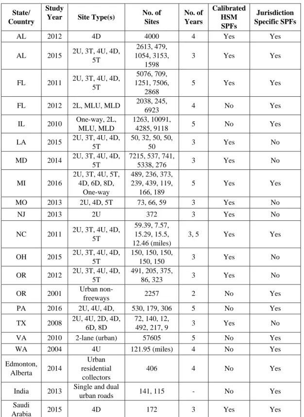
Table 2. Summary of studies involving calibration or development of specific SPFs (Savolainen et al. 2016)

State/ Country

Study

Year Site Type(s) No. of Sites No. of Years Calibrated HSM SPFs Jurisdiction Specific SPFs AL 2012 4D 4000 4 Yes Yes AL 2015 2U, 3T, 4U, 4D, 5T 2613, 479, 1054, 3153, 1598 3 Yes Yes FL 2011 2U, 3T, 4U, 4D, 5T 5076, 709, 1251, 7506, 2868 5 Yes Yes FL 2012 2L, MLU, MLD 2038, 245, 6923 4 No Yes IL 2010 One-way, 2L, MLU, MLD 1263, 10091, 4285, 9118 5 No Yes LA 2015 2U, 3T, 4U, 4D, 5T 50, 32, 50, 50, 50 3 Yes No MD 2014 2U, 3T, 4U, 4D, 5T 7215, 537, 741, 5338, 276 3 Yes No MI 2016 2U, 3T, 4U, 5T, 4D, 6D, 8D, One-way 489, 236, 373, 239, 439, 119, 166, 189 5 Yes Yes MO 2013 2U, 4D, 5T 73, 66, 59 3 Yes No NJ 2013 2U 372 3 Yes No NC 2011 2U, 3T, 4U, 4D, 5T 59.39, 7.57, 15.29, 15.5, 12.46 (miles) 3, 5 Yes Yes OH 2015 2U, 3T, 4U, 4D, 5T 150, 150, 150, 150, 150 3 Yes No OR 2012 2U, 3T, 4U, 4D, 5T 491, 205, 375, 86, 323 3 Yes No OR 2001 Urban non-freeways 2257 2 No Yes

PA 2016 2U, 4U, 4D, 530, 179, 306 5 No Yes

TX 2008 2U, 4U, 2D, 4D,

6D, 8D

72, 140, 12,

492, 217, 9 3 Yes No

VA 2010 2-lane (urban) 57605 5 No Yes

WA 2004 4U 121.95 (miles) 4 No Yes Edmonton, Alberta 2014 Urban residential collectors 406 4 No Yes

India 2013 Single and dual

urban roads 141, 115 - No Yes

Saudi

(23)

Six states did not calibrate the HSM models and just developed SPFs for their

jurisdictions. Seven states only calibrated the HSM models. Five states did both. Most states that estimated models for their jurisdictions used the same classification method as the HSM for developing their SPF models, where the facility type is given by the number of lanes followed by a U for undivided roadways, a T for undivided roadways with a two-way left-turn lane (TWLTL), and D for a divided roadway. Some states, such as Washington and North Carolina, did not give a number of sites used for the estimation of the models, but instead used roadway length to describe the datasets. Some states used very few sites, most notably Louisiana and Missouri using fewer than 75 sites for their calibrations, with as few as 32 segments for 3T roadways in LA.

2.2 Economic Analysis

In order to provide guidance on whether a safety measure is cost effective, the Federal Highway Administration (FHWA) outlines in their Highway Safety Improvement Program (HSIP) manual two methods of benefit/cost analysis that focus on lifetime cost savings and lifetime expenses (FHWA 2011). Both methods convert future value to present value using standard economic principles.

The uniform annual benefits method treats the benefit value as an annuity. The total annual benefits are multiplied by a factor to convert it from future payouts to current value. The following equations are used:

| , , 2.2

(24)

where:

present value of benefits

| , , multiplier to determine total present value of monthly benefits

i = discount rate

n = service life in years

This method is used when the benefits are fixed for every year. The discount rate can be the inflation rate, or the interest rate at which the money could be invested if not used. The service life in years is the number of years that the particular safety countermeasure will be in the field.

The second method is for non-uniform annual benefits. The following equation is used:

| , , 2.4

| , , 1 2.5

where:

i = discount rate

n = service life in years

The for each year must be calculated and then summed. This method is best used when the benefits change over time, such as the retroreflectivity of lane markings, which degrade over time and so have less of an impact on crashes as they grow older.

(25)

To quantify the economic impact of crashes for the benefit/cost analysis, the HSM presents a table of comprehensive crash costs, seen in Table 3 (FHWA, 2011). In addition to estimating SPFs for their jurisdiction, an agency can also provide their own estimates of crash costs to obtain a better estimate of the benefits of safety countermeasures.

Comprehensive crash costs include not only the property damage, but also cost of congestion, loss of productivity, court/legal costs, emergency responders, and more. The National Safety Council (NSC) estimates the cost of the crash on a per person basis, that is, there is a cost associated with each fatality, incapacitating injury, and so on (NSC, 2014). This makes it more difficult to apply these costs to a crash, as the SPFs only predict the number of crashes and, if SDFs are used, the maximum severity breakdown, not the number of people involved in the accident. As such, the average number of fatalities per crash, incapacitating injuries per crash, and so on would need to be calculated on a system level for the jurisdiction. The crash costs in Table 3 are per crash.

Table 3. Comprehensive Crash Costs by Severity Level (FHWA, 2016)

Injury Severity Level Comprehensive Crash Cost Fatality (K) $4,008,900

Incapacitating Injury (A) $216,000 Minor Injury (B) $79,000 Possible Injury (C) $44,900 Property Damage Only (O) $7,400

2.3 Existing Tools/Guidance

AASHTO summarizes some of the tools available that can be used to implement the HSM. The Crash Modification Factors (CMFs) Clearinghouse website can be used to locate

(26)

CMFs for numerous countermeasures that have been published in reports, papers, and journal articles. There are also various programs that are available to supplement the HSM.

SafetyAnalyst and the Interactive Highway Safety Design Model (IHSDM) both require large amounts of data in order to use effectively. SafetyAnalyst works with Part B of the HSM, which details the process to select locations based on metrics including crash rates and frequencies. The IHSDM works with the predictive methods found in Part C of the HSM. Included in the data needs for this program are roadway geometry in addition to traffic volume and crash data (AASHTO 2017).

The Michigan DOT utilizes a spreadsheet tool for conducting a time-of-return (TOR) analysis for candidate projects. This spreadsheet uses observed crash frequencies and AADT growth factors to calculate the time required for the savings from crashes prevented to meet or exceed the cost of implementation of the project. Three to five years of crash data are recommended for the TOR spreadsheet, as it uses only observed crash data at the location, which means it is also vulnerable to the short term fluctuations in crash rates. The

spreadsheet assumes a linear relationship between crashes and AADT, which, as covered earlier, is not necessarily an appropriate assumption.

The Minnesota DOT has developed a guidance document on conducting benefit/cost analysis for transportation projects. In the document, there is discussion on the various uses of a benefit/cost analysis and its uses in project planning, as well as in the design phase and construction planning. It is suggested that different alternatives, whether they are projects, countermeasures, or sites, be considered to determine which have benefits that are worth the investment. Other states, such as Ohio, use benefit/cost ratios when considering projects, but do not have published methods for how they calculate them (ODOT, 2017). California DOT

(27)

uses a spreadsheet tool to do life-cycle benefit/cost analyses. Their spreadsheet is very generalized. Given that it is designed to estimate the benefit/cost ratio and life-cycle costs for any type of construction or improvement project, it has many of possible inputs and uses historical crash data (CalTrans, 2017).

Data driven analysis for safety countermeasures have driven the use of SPFs in calculating safety effectiveness and the available tools and documentation show that there is interest in using the benefit/cost ratio when determining which projects should move forward at the planning stage. However, the existing tools rely primarily on historical crash

frequencies, with some integration of SPFs to conduct EB analyses. The amount of data required can be impractical for project-level planning efforts when a large amount of countermeasures are being considered. SPFs can provide a prediction for the number of crashes and, by calculating the effect of a safety countermeasure, can provide an estimate of the benefit/cost ratio with minimal data requirements, making this information accessible at the project planning stage. This project hopes to encourage the use of SPFs in the benefit/cost analysis at the planning stages by creating an easy to use tool that can calculate the

benefit/cost ratio for prospective projects quickly and can be easily modified to with locally calibrated SPFs.

(28)

CHAPTER 3: SPF AND SDF DEVELOPMENT

The accuracy of an SPF depends heavily on the quality and quantity of the data used to estimate it. More complex models that include a large variety of inputs in an effort to account for the many differences in roadway and traffic characteristics to adequately predict crashes, necessarily require a great deal of information regarding the roadway and traffic stream. When examining projects at the pre-feasibility level, it is not generally convenient to gather all of this information. However, it is possible to produce a simplified (and

generalized) SPF that might be less accurate for a particular road segment, but requires much less data to use for prediction. This technique is used for the models included in the

spreadsheet tool developed for this project. These SPFs use just 3 variables, AADT, length, and a regional indicator variable to account for general differences in crash expectancy across geographic regions. To calculate the economic impact of the crashes, SDFs were used to predict the distribution of crash severity. The SDFs used in this spreadsheet tool require a total of 3 inputs, which are speed limit, terrain type, and roadway division type. Facility type is an additional input that is used to select the particular model to be used and also

determines the roadway division type, allowing for only 2 manual inputs for use in the SDFs.

It would have been possible to utilize the general SPFs provided in the HSM. However, to demonstrate how this tool can be individualized for use in a particular

jurisdiction, SPFs have been developed for Michigan state-maintained urban and suburban roadways (that is, segments that are within the city limits of communities with a population of 5000 people or more). By predicting the number of crashes occurring on a roadway using very few variables, they allow the user to use the tool to quickly examine the benefit/cost ratio for a variety of safety countermeasures at a variety of locations, identifying those

(29)

candidates most suitable for future study with a minimum of cost and effort while still using data-driven analysis. Much of the framework developed for the tool and detailed in Chapter 4 was built around the variables used in these particular SPFs.

3.1 SPF Development

SPFs take the form of generalized linear models, with the negative binomial model being the framework most widely utilized in practice. Due to the nature of crash data, which are comprised of non-negative integers, regression techniques such as ordinary least-squares are typically inappropriate. There are many factors that influence crashes, including AADT, lane width, and others, and these factors do not necessarily have a linear relationship with crashes. As a measure of exposure, AADT is the backbone of an SPF and therefore can have a linear effect on crashes, but many times the relationship between the two will appear to follow more of an exponential fit. A simple linear least-squares regression would not

accurately capture these effects. Given the nature of crash counts as non-negative integers, a Poisson distribution provides a starting point for statistical analyses of crash data. However, a base assumption for a Poisson distribution is that the variance is equal to the mean. This is often not a valid assumption when looking at the frequency of crashes over a variety of road segments (such as all the roads in a state), as many segments will have few to no crashes while others will have an extremely high frequency of crashes. Because of this, the variance tends to be much higher than the mean, and the data are described as overdispersed as a result.

This violation of the Poisson assumption is controlled for by using a specific type of Poisson model, known as a negative binomial model (sometimes called a Poisson-gamma model). In this type of model, the single value Poisson parameter is replaced with a function.

(30)

The negative binomial model is recommended in the HSM for the development of SPFs and is used in the SPFs provided in that manual.

The SPFs used in the spreadsheet tool use the following equation:

∗ ∗ ∗ _3.1

where:

N = FI or PDO crashes per year

I = Intercept

= Regional indicator

= Coefficient for region

Both length and AADT were log-transformed during the estimation of the models and length was used as an offset variable, resulting in the equation in the form seen above. As an offset variable, the coefficient was fixed at 1.0. This introduces a practical constraint in that crashes are expected to change proportionately to segment length (i.e., if length doubles, crashes will double, as well). The regional indicators were included in these models because they can be used to capture regional differences without requiring the inclusion of a large number of variables. The regional differences can include weather (the amount of rain, snowfall, and plowing tendencies), roadway design (lane width, shoulder widths, and others), and driver behavior. This allows for improved model fit with a minimum number of inputs.

As crashes vary largely by facility type (the number of lanes and organization of those lanes), a separate SPF was estimated for each. Also, to facilitate later economic impact calculations, FI crashes and PDO crashes were estimated in separate models. This follows the

(31)

same procedure as the HSM. The intercept value in these models shifts the model up or down the vertical axis, in this case, increasing or decreasing the number of crashes that would ‘occur’ by a scalar. Although the value of the intercept does not have very much practical meaning in and of itself, it is important to include in the model as failure to do so may result in biased parameter estimates. The remaining coefficients represent the impacts of specific variables on the total number of crashes and must be remembered in the context of Equation 3.1. AADT coefficients are the power to which the AADT value is raised. If the coefficient is equal to 1.0, then crashes will increase directly in proportion to AADT. If the coefficient is less than one, as AADT increases, the rate at which crashes increase will slow. If the coefficient is greater than one, as AADT increases, the rate at which crashes increase will grow. Coefficients of 1.0 or greater are termed elastic with respect to AADT. AADT has also been shown to be inelastic in some contexts where crashes increase at a lesser rate as AADT increases (i.e., when the coefficient is less than 1.0). For the regional indicator coefficients, the sign indicates whether that region experiences more or fewer crashes in general than the Metro region (which was used as the base case to avoid over constraining the model). The magnitude of the coefficient indicates relative differences in safety performance on segments between that region and the Metro region.

A model was estimated for each individual facility type. Facility types are designated based on the number of lanes on the roadway as well as the configuration of those lanes. They are given in the form of a number followed by one of 3 letters. The number represents the number of lanes. The 3 possible letters are ‘U’, ‘T’, and ‘D’. ‘U’ stands for an undivided roadway, with a yellow centerline. ‘T’ stands for a roadway with a TWLTL in place of a yellow centerline. ‘D’ stands for a divided roadway, where some barrier is in place between

(32)

the lanes going in opposing directions. Images of the different facility types can be found in Figure 9 in section 4.1.1.

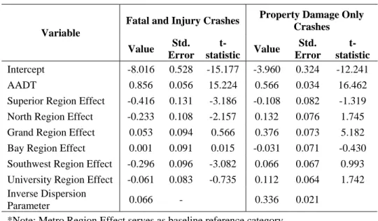
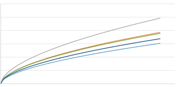
For 2U segments, the FI crashes tend to be more elastic with AADT than the PDO crashes, as can be seen by the coefficients in Table 4. The regional effects also differ between FI and PDO. Of particular note is the fact that the signs of several of the regional indicators change between FI and PDO crashes. For example, the coefficient for the North region is -0.233 for FI crashes (meaning there are fewer FI crashes with respect to AADT compared to the Metro region) and 0.132 for PDO crashes (meaning there are more PDO crashes with respect to AADT compared to the Metro region). This change can be seen in the graphs below. In Figure 2, the orange line that shows the crashes per mile in the North region is below the blue line that represents crashes per mile in the Metro region (base case). In Figure 3, the orange line for the North region is above the blue line that represents crashes per mile in the Metro region. This shows the differences that can appear between the two types of crashes and highlights the need to model them separately.

(33)

Table 4. SPF for Crashes on 2U Segments with AADT and Regional Indicators

Variable

Fatal and Injury Crashes Property Damage Only Crashes Value Std. Error t-statistic Value Std. Error t-statistic Intercept -8.016 0.528 -15.177 -3.960 0.324 -12.241 AADT 0.856 0.056 15.224 0.566 0.034 16.462

Superior Region Effect -0.416 0.131 -3.186 -0.108 0.082 -1.319

North Region Effect -0.233 0.108 -2.157 0.132 0.076 1.745

Grand Region Effect 0.053 0.094 0.566 0.376 0.073 5.182

Bay Region Effect 0.001 0.091 0.015 -0.031 0.071 -0.430

Southwest Region Effect -0.296 0.096 -3.082 0.066 0.067 0.993

University Region Effect -0.061 0.083 -0.735 0.112 0.064 1.742

Inverse Dispersion

Parameter 0.066 - 0.336 0.021

*Note: Metro Region Effect serves as baseline reference category

Figure 2. FI Crashes per Mile for 2U Segments with Regional Effects

0 0.5 1 1.5 2 2.5 0 5000 10000 15000 20000 25000 30000 35000 C rashes per M il e AADT

(34)

Figure 3. PDO Crashes per Mile for 2U Segments with Regional Effects

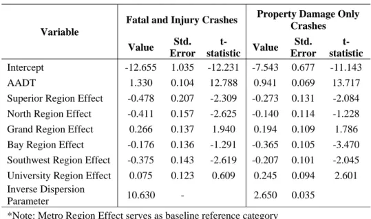
For the 4U segments, PDO crashes are fairly elastic with AADT, but as AADT increases, the rate of FI crashes also increases (coefficient is greater than 1). This can be seen in the slopes of the lines in Figure 4. While the PDO line reaches a higher number of crashes, its slope is mostly linear, with a slight tendency towards concave down. The FI line, on the other hand, has a distinct concave up shape. The regional effects for this facility type are more consistent, with no coefficients changing signs. The coefficients can be found in Table 5. 0 2 4 6 8 10 12 0 5000 10000 15000 20000 25000 30000 35000 C rashes per M il e AADT

(35)

Table 5. SPF for Crashes on 4U Segments with AADT and Regional Indicators

Variable

North Region Effect -0.411 0.157 -2.625 -0.140 0.114 -1.228

Bay Region Effect -0.176 0.136 -1.291 -0.365 0.105 -3.470

Southwest Region Effect -0.375 0.143 -2.619 -0.207 0.101 -2.045

University Region Effect 0.075 0.123 0.609 0.245 0.094 2.601

Inverse Dispersion

Parameter 10.630 - 2.650 0.035

Figure 4. Annual Crashes per Mile for 4U Segments in Metro Region

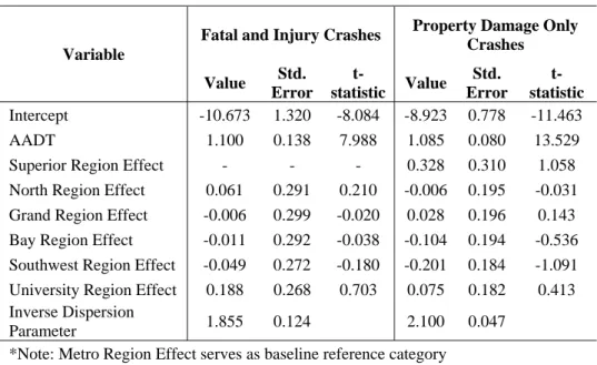
The relationship between AADT and crashes is more uniform between FI and PDO crashes for the 3T facility type. Both crash types are very elastic with regards to AADT as well. The coefficients are in Table 6.

0 2 4 6 8 10 12 14 16 0 5000 10000 15000 20000 25000 30000 35000 40000 45000 50000 C rashes per M il e AADT FI PDO

(36)

Table 6. SPF for Crashes on 3T Segments with AADT and Regional Indicators

Variable

Superior Region Effect - - - 0.328 0.310 1.058

North Region Effect 0.061 0.291 0.210 -0.006 0.195 -0.031

Grand Region Effect -0.006 0.299 -0.020 0.028 0.196 0.143

Bay Region Effect -0.011 0.292 -0.038 -0.104 0.194 -0.536

Inverse Dispersion

Parameter 1.855 0.124 2.100 0.047

For both FI and PDO crashes, the graph is concave up. All but the Superior region have positive coefficients for the regional indicators for the 5T facility type, as seen in Table 7.

Table 7. SPF for Crashes on 5T Segments with AADT and Regional Indicators

Variable

North Region Effect 0.040 0.096 0.418 0.366 0.075 4.880

Bay Region Effect 0.057 0.080 0.717 0.243 0.063 3.876

Southwest Region Effect 0.086 0.083 1.035 0.295 0.065 4.545

Inverse Dispersion

Parameter 2.910 0.032 2.202 0.022

(37)

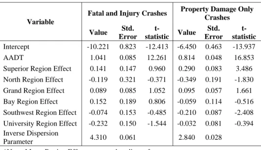
For the 4D segments, FI crashes are elastic with AADT, but PDO crashes are somewhat inelastic with that variable. The coefficients can be found in Table 8.

Table 8. SPF for Crashes on 4D Segments with AADT and Regional Indicators

Variable

Superior Region Effect 0.141 0.147 0.960 0.290 0.083 3.486

North Region Effect -0.119 0.321 -0.371 -0.349 0.191 -1.830

Bay Region Effect 0.152 0.189 0.806 -0.059 0.114 -0.516

University Region Effect -0.232 0.150 -1.544 -0.032 0.081 -0.394

Inverse Dispersion

Parameter 4.310 0.061 2.840 0.028

The effect of AADT on the crashes for 6D segments results in a concave up graph shape, as can be inferred from the coefficients in Table 9.

Table 9. SPF for Crashes on 6D Segments with AADT and Regional Indicators

Variable

Superior Region Effect - - - -

North Region Effect - - - -

Bay Region Effect - - - -0.074 0.497 -0.149

Southwest Region Effect 0.036 0.744 0.048 -0.073 0.458 -0.159

University Region Effect -0.518 0.272 -1.906 -0.339 0.162 -2.090

Inverse Dispersion

Parameter 2.690 0.073 1.740 0.057

(38)

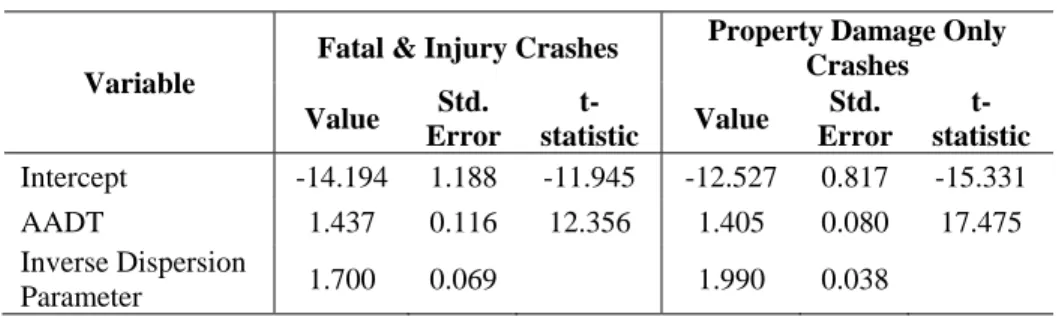
Due to a lack of 8D segments outside the Metro region, regional effects were not estimated for this facility type. The coefficients in Table 10 represent the AADT only model for 8D segments. The high coefficient for AADT shows a strong relationship between AADT and crashes.

Table 10. SPF for Crashes on 8D Segments with AADT

Variable

Fatal & Injury Crashes Property Damage Only Crashes Value Std. Error t-statistic Value Std. Error t-statistic Intercept -14.194 1.188 -11.945 -12.527 0.817 -15.331 AADT 1.437 0.116 12.356 1.405 0.080 17.475 Inverse Dispersion Parameter 1.700 0.069 1.990 0.038 3.2 SDF Development

The SDFs were developed generically for the two way urban and suburban trunkline system as part of a project for Michigan DOT (Savolainen et al. 2016). The SDFs can be used to estimate the proportion of crashes that result in specific injury severity levels based on the KABCO scale. For this scale, K represents a fatal crash where at least one person involved in the crash was killed, A represents an incapacitating injury, B represents a non-incapacitating injury, C represents possible injury, and O is a property-damage-only (or no-injury) crash. This determination is made by the police officer responding to the crash and is recorded in the crash reporting form. The SDFs use some geometric characteristics to individualize the estimated proportions to the site.

A multinomial logit (MNL) model was used to estimate the probabilities. The following equations were used:

(39)

K P ₌ B A K K V V V V e e e e    1 3.2 A P ₌ B A K A V V V V e e e e    1 3.3 = K A B B V V V V e e e e    1 3.4 = 1 PK  PA  PB 3.5 where: j

P

= probability of the occurrence of crash severity j;

j

V

= systematic component of crash severity likelihood for severity j.

The following equations were used to calculate the components of the above equations: K V ₌

_ASC

_b

_I

_b

_I

_b

_PSL

K psl div K div ter K ter K



,





,





,



3.6 A

V ₌

ASC

_A



b

_ter_,_A



I

_ter



b

_div_,_A



I

_div



b

_psl_,_A



PSL

3.7

B

V ₌

ASC

_B



b

_ter_,_B



I

_ter



b

_div_,_B



I

_div



b

_psl_,_B



PSL

_3.8

where:

ter

I

= terrain indicator variable (=1.0 if level, 0.0 if it is rolling);

div

I

= divided road indicator variable (=1.0 if divided, 0.0 otherwise); PSL _{= posted speed limit on the segment, miles per hour;}

= alternative specific constant for crash severity j; and = calibration coefficient for variable k and crash severity j.

The parameter estimates for the SDFs are severity specific. The variables included in this model provided the best fit for the data while at the same time being logical. The

B P C P j ASC j k b_,

(40)

variables included for consideration were the variables that, considered when developing a fully specified model, had an impact on crashes. The coefficients can be found in Table 11.

Table 11. Parameter estimation for SDFs (Savolainen et al. 2016)

Coefficient Variable Fatality (K) Incapacitating injury (A) Non-Incapacitating injury (B) Value t-statistic Value t-statistic Value t-statistic ASC Alternative specific constant -4.930 -7.49 -2.631 -8.28 -1.427 -6.99 ter

b

Terrain (1=level; 0=rolling) -0.656 -2.54 -0.256 -1.69 -0.130 -2.53 div

b

Divided road (1=divided; 0=others) -0.355 -1.99 -0.354 -4.16 -0.130 -2.53 PSL Posted speed limit, mph 0.042 3.49 0.018 3.28 0.013 3.74 Observations 10,021 crashes (K=173; A=809; B=2,340; C=6,699)

(41)

CHAPTER 4: TOOL DEVELOPMENT

For a tool to be valuable, accessibility and ease of use are two of the main concerns that must be considered. Although SPFs and SDFs can provide a solid statistical basis for evaluating the effect of safety countermeasures – something that matters as transit agencies seek to use data to drive the decision making process – the complexity of the statistical equations can be a concern when it comes to usability. As described in Chapter 2, tools for using the methods in the HSM exist, but they require large amounts of data. Therefore, this tool was developed in order to leverage the advantages provided by using SPFs and SDFs at the pre-feasibility stage while reducing the complexity of running comparisons.

Rather than write a stand-alone program, the decision was made to use a common spreadsheet program as the tool framework. This software is widely prevalent and most users will already be familiar with basic operations, reducing the learning curve and achieving the goal of making the tool accessible and easy to use. This tool is intended for use as a project-level planning tool to do simple pre-feasibility analyses. It calculates a benefit/cost ratio based on the SPFs loaded into it. It does not calculate time of return, nor does it utilize observed crashes. The predictive models included in the model were developed using data from Michigan state-maintained urban and suburban non-interstate roadways. The underlying SPFs can be modified to allow other jurisdictions to utilize the framework for their own roadways.

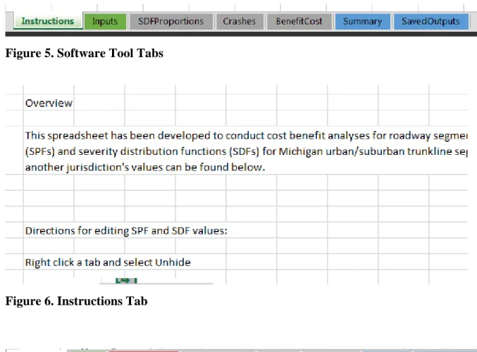
The spreadsheet consists of multiple tabs, as seen in Figure 5. The Instructions tab (Figure 6) details the process of how to modify the predictive equations to suit the

jurisdiction. The Inputs tab prompts for the inputs necessary to estimate the benefit/cost ratio of the countermeasure. Intermediate calculations are presented in the SDF Proportions,

(42)

Crashes, and Benefit/Cost tabs. Finally, the Summary and Saved Outputs tabs display the results of the analysis. The Tables and Lists tab, normally hidden from the user (displayed visibly in Figure 7), contains the coefficients for the predictive equations, various lists, and a series of helper cells.

Figure 5. Software Tool Tabs

Figure 6. Instructions Tab

Figure 7. Software Tool Tabs with Tables and Lists

4.1 Inputs

The inputs tab (pictured in Figure 8) asks for three 3 different types of information from the user: roadway and traffic characteristics, safety countermeasure/treatment

(43)

Figure 8. Inputs Tab

4.1.1 Roadway/Traffic characteristics

The first input for the roadway and traffic characteristics is facility type. As discussed in Chapter 3, this refers to the number of lanes and configuration of those lanes. The models preset in the spreadsheet tool are for Michigan urban and suburban trunkline segments, which have facility types ranging from 2U to 8D. Figure 9 contains examples of each facility type.

(44)

2 Lane Undivided (2U) 3 Lane with a TWLTL (3T)

4 Lane Undivided (4U) 5 Lane with a TWLTL (5T)

4 Lane Divided (4D) 6 Lane Divided (6D)

8 Lane Divided (8D)

(45)

In the Inputs tab, facility type is selected using a dropdown list, as shown in Figure 10. Facility type is extremely important for the tool, as it dictates which SPF is used for calculating crashes and is used to set the divided roadway variable in the SDF. By using a dropdown list, the inputs are standardized, allowing the formulas embedded in the

spreadsheet to reference other values based on facility type, which is particularly important for the SPFs as discussed in Chapter 3. The list of facility types for the dropdown menu can be changed if necessary and is pulled from the tables and lists tab.

Figure 10. Facility Type Dropdown Menu

The next input, Region, also utilizes a dropdown menu for consistency and for ease of use. By using the dropdown menu, the user will not have to remember which regional

identifiers were used in order to select the appropriate regional coefficients. The input options can be seen in Figure 11. Like the facility type dropdown, this list is pulled from the tables and lists tab. As discussed in section 3.1, region was chosen as the 3rd variable in the SPF (after AADT and length) because it captures some of the differences in roadway design between areas of the state, such as lane and shoulder widths, weather, and driver behavior.

(46)

Figure 11. Region Dropdown Menu

AADT, the next input, is a numeric value from the analyst. Values for this cell have been restricted to integers greater than 0. If the AADT input is greater than 80,000, the cell will turn red to indicate that an AADT far outside the model ranges has been entered and the results should be treated with caution. Table 12 contains the model AADT ranges, rounded down to the nearest 100 for the minimums and up to the nearest 100 for the maximums.

Table 12. Model AADT Ranges

Facility Type Min AADT Max AADT

2U 200 30200 3T 2400 31100 4U 3700 43900 5T 4100 51300 4D 1800 35900 6D 3400 77600 8D 6000 77600

A dropdown menu with 2 choices is the input for Terrain type, used in the SDF calculations. The options for this are Level and Rolling. The spreadsheet tool menu can be seen in Figure 12. Examples of level and rolling terrain can be seen in Figure 13. Crashes on rolling terrain tend to be more severe, which matters when considering the economic impact of a safety countermeasure.

(47)

Figure 12. Terrain Dropdown Menu

Figure 13. Level (left) and Rolling (right) Terrain

The next input is the speed limit of the road. Like AADT, this is a numeric input from the analyst. The value input into this cell is restricted to integer values between 15 and 85 miles per hour. This range can be modified in the future if higher speed limits are introduced. Details on the modification process can be found in chapter 5.

The length of the road is the final input in the roadway and traffic characteristics. Road length here measures the segment length that the safety countermeasure is being considered on and is given in miles.

4.1.2 Safety countermeasure/treatment

The first input for the safety countermeasure/treatment characteristics is the CMF. There are 3 different ways to use CMFs with the spreadsheet tool. A dropdown menu allows the analyst to select one of these 3 options: Preset, Input Single Value, and Input Severity Specific. Figure 14 shows this menu. Depending on the input method selected, different rows

(48)

are visible. Selecting Preset displays a row with a 2nd_{dropdown menu that contains several} preset CMFs, taken from CMF Clearinghouse. The values included for cable median barrier come from 2 different studies (Elvik, 2004; Olson et al. 2013). The 4U to 3T lane diet CMF came from an EB study (Persaud et al., 2010). The rumble strips CMF comes from a NCHRP report (Torbic et al., 2009). More CMFs can be added as they are developed. If the

jurisdiction develops CMFs for countermeasures in their area, these can be used in place of values from the CMF Clearinghouse. This list can be seen in Figure 15. Modifying the values available will be discussed in Chapter 5. Selecting Input Single Value provides a row labeled ‘Single Value’ for the input of the relevant CMF, as shown in Figure 16. Selecting Input Severity Specific displays a series of rows where CMFs can be manually input for crashes on the KABCO severity scale, as seen in Figure 17.

Figure 14. CMF Dropdown Menu

(49)

Figure 16. Input Single Value

Figure 17. Input Severity Specific

The next inputs have to do with the cost of installing and maintaining the proposed countermeasure. During the development of the tool, incorporating the cost values into the presets with the CMFs was considered. However, due to vastly differing costs across the country, and the desire to have this tool be usable easily by any jurisdiction, it was

determined that leaving the cost values as an input for the analyst would allow for the most flexibility for the tool. The first of these two inputs calls for the capital expense cost per mile, or the initial installation cost. The second of these two inputs calls for the yearly maintenance cost per mile. As with the capital expense cost, this is left as a numeric input by the analyst. The values for these two cells are restricted to values greater than 0 for the capital expense and greater than or equal to 0 for the maintenance cost. The values seen in the sample input in Figure 8 are for cable barrier installation in the Greater Minnesota area. As of December 2016, the Minnesota DOT estimated that cable barrier cost $140,000 to $150,000 per mile to install and $6000 per mile per year in maintenance (MnDOT 2016).

(50)

The decimal discount rate is another analyst input, which is used to allow for inflation to be taken into account when looking at the value of the benefits and costs in the future. Default values for this field can range from 0.025 to 0.04.

Service life is the final input used in calculations. The number of years that a countermeasure is in the field determines the total cost of the countermeasure (given the maintenance costs) as well as the total benefit (given the crashes prevented each year).

4.1.3 Analysis information

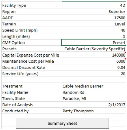
This group of inputs, seen in Figure 18, is used for identification of the site in question and the person who is running the analysis. The first input is the name of the

treatment being considered. This allows easy identification of which countermeasure is being evaluated for a given benefit/cost ratio in the saved outputs tab for later comparison. The next field is for facility name. This can be however specific the analyst desires. The 3rd_{field is the} town and state where the facility is located. This information can be used in conjunction with the previous input to determine the specific street. The 4th field is the date the analysis was conducted. The final input is the name of the analyst.

(51)

4.2 Calculation Tabs

This series of tabs is used for the intermediate calculations. The proportions of crashes for each severity level are determined on the SDF Proportions tab as seen in Figure 19. Values from the inputs are inserted into the SPF equations from chapter 3 to calculate the predicted crashes on the Crashes tab, Figure 20. The CMFs are also applied on that tab. The net change in crashes is then used to calculate the total comprehensive crash costs associated with the countermeasure on the BenefitCost tab (Figure 21) and present values of the benefits and costs are determined. The following sections will go into more detail on what the tabs contain.

4.2.1 SDF proportions

This tab (shown in Figure 19) calculates the proportions of FI crashes that fit into each severity type on the KABCO scale. Using the models presented in section 3.2, the values of the utility functions for K, A, and B crashes are calculated. Following that, the proportions of the K, A, and B crashes can be calculated. The proportion of C crashes is found by subtracting the proportions of the other 3 severities from 1.

(52)

4.2.2 Crashes

This tab (displayed in Figure 20) contains the calculations for the SPFs. PDO crashes and FI crashes are calculated based on the inputs outlined in section 4.1. Using these

numbers, the total crashes are calculated. Once the total crashes predicted are known, it applies the CMFs. In the cases where a single CMF applies to all severity types, then the one value is multiplied to each of the predicted crashes. In the cases where there are severity specific CMFs, the appropriate CMF value is multiplied to each severity. After the predicted crashes post countermeasure installation are calculated, the total crashes reduced are

determined by subtracting the post CMF crashes from the predicted totals.

Figure 20. Crashes Tab

4.2.3 BenefitCost

The BenefitCost tab (pictured in Figure 21) shows the calculations for the benefit/cost ratio. First, the monetary value of the crashes after the safety countermeasure is installed is calculated. In cases where the treatment increases crashes for some severity levels, these

(53)

values will be negative. The total of the values is the present value of the crashes per year. To compare all costs and benefits in the current year, a formula is used that calculates a

multiplier for the present value of an annuity given the number of years and an interest rate (FHWA 2016). These values are taken from the inputs, as the service life of the

countermeasure and the discount rate. The formula used is as follows:

| , , _∗ 4.1

where:

I = discount rate

n = service life

The result of this equation, (P|A,I,n), is multiplied to the present value for 1 year to calculate the total value over the service life. The same value is multiplied to the maintenance cost, to determine the present value of the yearly maintenance. The present value of the benefits and the present value of the costs are both summed. The benefit value is then divided by the cost value to determine the benefit cost ratio.

If this value is greater than 1, then from an economic standpoint, the safety

countermeasure being examined would be a net benefit. The larger the number, the greater the benefit is in comparison to the cost of implementation and maintenance. If this value is less than one but is still positive, then the costs outweigh the benefit and the countermeasure is not feasible from an economic standpoint. If the value is negative, then there is no

(54)

Figure 21. BenefitCost Tab

4.3 Tables and Lists

The backbone of the spreadsheet is the Tables and Lists tab (excerpt in Figure 22), which contains all the lists and cell references used to make the spreadsheet work. Changes to this spreadsheet are unnecessary for normal use, except when modifying the tool to use SPFs and SDFs calculated for the local area, and have the potential to break the tool if changed accidentally. However, it is not possible to lock this spreadsheet to prevent accidental editing (as is done for the calculations tabs) because the user does need the

capability to edit this spreadsheet in order to modify the tool for their jurisdiction. Therefore, the tab is simply hidden from view during normal use.

(55)

This tab contains all the lists used for the dropdown menus in the Inputs tab. The coefficients for the SPFs and SDFs are present in this tab as well. All the cell references between sheets are done using named cell ranges, for reasons discussed in Chapter 5.

Figure 22. Section of Tables and Lists Tab

4.4 Output Tables

The summary table presents the results of the calculations, as seen in Figure 23. The analysis information (from section 4.1.3) is all listed in the summary table, as well as the benefit/cost ratio, present value of both the benefits and the costs, the net changes in crashes, and the AADT and length values, as well as the service life and discount rate used. Included on the tab are 3 buttons. The first button, labeled ‘Copy Data to Saved Outputs’ does exactly that. Pressing it copies the formatting and values of the summary table to the saved outputs tab. The second button, labeled ‘Go To Saved Outputs’ makes the Saved Outputs tab the active tab. The third button, ‘Return to Inputs’, makes the Inputs tab the active tab. These buttons are used to make it easier to navigate between tabs, as well as save the data from the summary table so that more iterations can be completed.

Development of a framework to compare the cost-effectiveness of traffic crash countermeasures