An Accelerated MDM Algorithm for SVM
Training
´
Alvaro Barbero, Jorge L´opez, Jos´e R. Dorronsoro∗
Dpto. de Ingenier´ıa Inform´atica and Instituto de Ingenier´ıa del Conocimiento Universidad Aut´onoma de Madrid, 28049 Madrid, Spain
Abstract. In this work we will propose an acceleration procedure for the Mitchell–Demyanov–Malozemov (MDM) algorithm (a fast geometric algo-rithm for SVM construction) that may yield quite large training savings. While decomposition algorithms such as SVMLight or SMO are usually the SVM methods of choice, we shall show that there is a relationship between SMO and MDM that suggests that, at least in their simplest implemen-tations, they should have similar training speeds. Thus, and although we will not discuss it here, the proposed MDM acceleration might be used as a starting point to new ways of accelerating SMO.
1
Introduction
The standard formulation of SVM training seeks to maximize the margin of a separating hyperplane by minimizingkWk2/2 subject toyi(W·X
i+b)≥1, i= 1, . . . , N; we assume a linearly separable training sample S = {(Xi, yi)} with
yi = ±1. Any pair (W, b) verifying the previous restrictions is said to be in canonical form. However, in practice the problem actually solved is the simpler dual problem of maximizing LD(α) = Piαi−12
P
i,jαiαjyiyjXi·Xj subject now to αi ≥ 0,
P
iαiyi = 0. The optimal weight Wo can be then written in the so–called dual form asWo =Pαo
iyiXi and patterns for which αoi >0 are called support vectors (SV). Among the many methods proposed to maximize
LD(α), Joachim’s SVMLight [1] is probably the fastest one. It repeatedly solves simpler maximization problems working with a restricted set ofqcandidate SVs. Whenq= 2 these reduced problems can be solved analytically and SVMLight coincides then with Platt’s SMO algorithm [2], also a popular, efficient and quite simple algorithm.
SVM training can also alternatively cast [3] as a Nearest Point Problem (NPP), where we want to find the closest points W∗
± in the convex hulls of the
positive (i.e.,y= 1) and negative samples. More precisely we want to minimize
kW+−W−k2= P i,jαiαjyiyjXi·Xjwhere PN i=1αi= 2, PN i=1yiαi= 0αi≥0. If we work with a zero bias term b (which can be compensated working with extended vectors X0 = (X,1)), NPP can be further reduced [4] to a Minimum
Norm Problem (MNP), where we want to find the vectorW in the convex hull
C( ˜S) of the set ˜S with the smallest norm. More precisely, we want to minimize nowkWk2=P
i,jαiαjyiyjXi·Xj with
PN
i=1αi= 1, αi≥0.
∗With partial support of Spain’s TIN 2004–07676 and TIN 2007–66862 projects. The first
MNP is a much older problem than SVM training and two algorithms to solve it have been adapted to SVM construction, the Gilbert–Schlesinger–Kozinec (GSK) [5, 6, 4] and the Mitchell–Demyanov–Malozemov (MDM) [7, 6]. The MDM algorithm iteratively updates a weight vectorWt=
P αt
jyjXj, selecting two vectors Xt
L = arg min{yjWt·Xj},XUt = arg max
©
yjWt·Xj, αtj>0
ª
, at each step and updating Wt to Wt+1 =Wt+λt(yLtXLt −yUtXUt) =Wt+λtDt, where λt= min ½ αt U, −Wt·Dt kDtk2 ¾ = min ½ αt U, ∆t kDtk2 ¾ .
These updates can be expressed in terms of theαmultipliers asαt+1
L =αtL+λt,
αtU+1 = αt
U −λt, αti+1 = αti ∀i 6= L, U. We note in passing that the above formulae allow an easy kernel extension of the MDM algorithm that only requires keeping track of theαt
j coefficients, the approximate marginsdtj =yjWt·Xj and the normskWtk2. Observe that ifλt=αtU,αtU+1= 0. Thus, the MDM algorithm can remove previous wrong SV choices (something that GSK cannot).
At first sight, one could look at the MDM algorithm as too far away from state–of–the–art SVM training methods such as SVMLight or SMO. However, notice that at each step MDM chooses two updating vectors XL and XU and adjusts two multipliers, just as SMO does. Thus, an alternative way of solving the MNP problem could be to proceed a la SMO. In fact, we shall show in section 2 that, after minor simplifications, doing so results in just the MDM algorithm. While much faster than GSK, in some problems MDM may also require too many iterations for wrong SV removal (see figure 1). In this work we propose a procedure to accelerate MDM training in which we detect the possible presence of training “cycles” and use them to construct a better updating vector. Although those updates have a higher computational cost than the standard ones, we shall illustrate in section 4 that significant training savings can be achieved. Moreover, the previously mentioned MDM-SMO relationship suggests that similar procedures could be successfully applied to accelerate SMO SVM training. We will not, however, discuss them here, and the paper will end with a short conclusion and some pointers to further work.
2
MDM and SMO
As just mentioned, one possibility when solving MNP could be to do it a la SMO; that is, to work at each step with two coefficients that we denote asαi1,αi2, fixing
all the otherαj and arriving at an analytical solution for this restricted version of MNP. The new multipliers to be considered are thus α0
i1 =αi1 +δi1, α
0
i2 =
αi2+δi2 andα
0
j=αj for all other. In dual form, the new vectorW0 considered has thus the form W0 = W +δ
i1yi1Xi1 +δi2yi2Xi2. While several different
heuristics can be used in SMO to choose the first coefficientαi1 [8], the second
multiplierαi2 is selected so that there is a maximum decrease inkW
0k2. Taking
into account the restrictionPiα0
i= 1, we must have δi2=−δi1 and, therefore,
we have W0 =W +δ
i1(yi1Xi1−yi2Xi2) = W +δi1D and kW
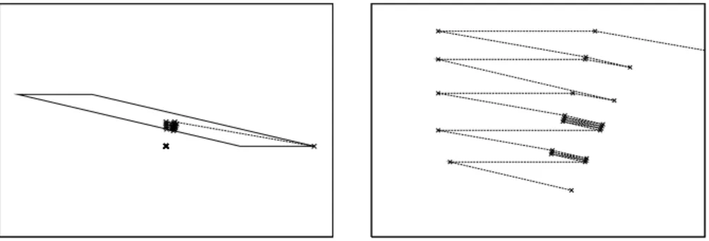
Fig. 1: The MDM algorithm may require many iterations even in simple prob-lems. However (right) they may have a cyclical structure.
2δi1W ·D+δi21kDk
2 = Φ(δ
i1), where D =yi1Xi1 −yi2Xi2. The last equation
implies that the optimalδ∗
i1 is given byδ
∗
i1=−W·D/kDk
2. In turn, this yields
Φ(δ∗
i1) =kW+δ
∗
i1Dk
2=kWk2−(W·D)2/kDk2. Thus, once the multiplierα
i1
has been chosen, we can selecti2 as i2 = arg maxjn(W·Dj)2/kDjk2
o
, where
Dj =yi1Xi1−yjXj. We can simplify the choice ofi2if we drop the denominator
kDjk2, selecting theni2 as
i2= arg maxjn(W·Dj)2
o
= arg maxj{|W ·(yi1Xi1−yjXj)|}.
The usual choice in SMO forαi1 is to take as the vectorXi1 the one that most
violates the KKT conditions. It is not clear how to bring this to an MNP setting but a way of doing so is to observe that the patternXi1 for which the KKT
con-ditions are violated most is the one that sets the margin of the current vectorW
and that, moreover, the SMO update will improve the margin of the new vector
W0 at the selectedX
i1. The same heuristic can be applied in the MNP setting
if we choosei1 = arg mini{yi(W·Xi)}. Now, since we also want to maximize
|W ·(yi1Xi1 −yjXj)|, we can simply take i2 = arg maxj{yjW·Xj}. Further-more, the optimal δ∗
i1 becomes now δ ∗ i1 = −W ·D/kDk 2 > 0, and, therefore, δ∗ i2 = −δ ∗
i1 < 0. Since we must ensure that α
0
i2 remains positive, αi2 must be
positive to begin with. Hence, we have to slightly refine our selection of i2 to
i2 = arg maxj,αj>0{yjW ·Xj}. Now, and as discussed in the previous section,
the choices for i1 and i2 are exactly the updates that are used in the bias-free MDM problem, i.e., we haveL=i1, U =i2. In other words, solving the MNP problem a la SMO yields the MDM algorithm.
3
Update Cycles in MDM Training
The main reason for the slow convergence of the GSK algorithm is that it requires many iterations to remove a wrong initial choiceXi of a support vector, i.e., to
BCW HD GCr PID Ban Thy Spl 2σ2 104 103.5 103 102 1 1 101.5
C 10 10 1000 10 10 101.5 1
Table 1: SVM 2σ2 andC parameters used.
achieve αi = 0. On the other hand, we can remove a SV Xi2 in the MDM
algorithm if we would have δ∗
i2 = W ·D/kDk
2 = −α
i2. However, this is not
guaranteed to happen and, in fact, wrong initial choices of support vectors may also be hard to correct by the MDM algorithm. This is shown in figure 1: it is clear that the optimalW∗ must be placed on the rhomboid face closer to 0;
however, if we start the MDM iterations on the lower right vector, it may take quite a few iterations before the MDM updates reach that face. In other words, the MDM will eventually reach the appropriate lower dimensional face removing thus the wrong initial vector choice, but quite often after many iterations as those described in figure 1, right.
The zigzags in that figure illustrate the more general presence of cycles within MDM training, where if a certain update vectorDT has reappeared afterKsteps from a former instance DT−K, it is likely that, somewhere later in training, the intermediate updates DT−j,1 ≤ j ≤K−1, will also be repeated, that is
Dt−j =DT−jfor somet > T. For instance, this is what happens in figure 1, that also suggests a possible way out of this. Notice that if we usedV =λ1D1+λ2D2, with D1, D2 the first updates in figure 1, right, as an updating direction, we could reach the right face in a single update minimizing kW2+λVk2. Once
there, just another step brings us to the optimalW∗. For a more general cycle
DT−K, DT−K+1, . . . , DT−1, DT =DT−K, we could defineV =
PK
j=1λT−jDT−j and, instead of the MDM standard update, consider one of the form WT+1 = WT+λTV, whereλT minimizes the normkWT+λVk2. It can be easily seen that the optimal λT is given by λT = −WT ·V /kVk2. These new updates require the efficient computation of WT+1 ·V and kVk2, as well as that of the new
coefficientsαTj+1 and approximate marginsdjT+1=yjWT+1·Xj.
LetI ={i1, . . . , iM}be the index set of those patternsXih that appear as
ei-therXLorXUinV. We have thenV =
PK j=1λT−j ³ yTL−jXLT−j−yUT−jXUT−j ´ = PM
h=1µhyihXih , where for T −K ≤ p, q ≤ T −1 we use the notation µh = P
Xih=Xp Lλp−
P
Xih=Xq
Uλq. It is clear now thatkVk 2=P
m,nµmµnyimyinXim· Xin. As for the newd
T+1
j , we havedTj+1=yjWT+1·Xj and, hence,
dTj+1=yjWT ·Xj+yjλT M X h=1 µhyihXih·Xj.=d T j +yjλT M X h=1 µhyihXih·Xj. Finally,PjαTj+1yjXj =WT+1=WT+λTV = P jαTjyjXj+λT PM h=1µhyihXih,
and it follows that αTj+1 = αTj ifj /∈ I, αiTh+1 = α
T
Std. MDM Accel. MDM
Dataset # KOs # iters. # KOs # iters. # KO reduct.
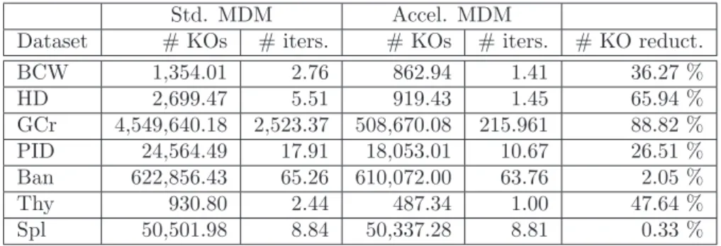
BCW 1,354.01 2.76 862.94 1.41 36.27 % HD 2,699.47 5.51 919.43 1.45 65.94 % GCr 4,549,640.18 2,523.37 508,670.08 215.961 88.82 % PID 24,564.49 17.91 18,053.01 10.67 26.51 % Ban 622,856.43 65.26 610,072.00 63.76 2.05 % Thy 930.80 2.44 487.34 1.00 47.64 % Spl 50,501.98 8.84 50,337.28 8.81 0.33 %
Table 2: Average number of kernel operations and iterations (both in thousands) for the standard and accelerated MDM algorithm and % reduction in kernel operations achieved by the second method.
updates must also verify 0 ≤ αT+1
ih = α
T
ih+λTµih ≤ 1. If µih > 0, the
rele-vant bound is the upper one, while the lower one has to be checked ifµih <0.
This implies that for these special cycle updates we must clipλT from above as
λT ≤min
©
(1−αT
ih)/µih :µih >0 ª
and also asλT ≤min
© −αT
ih/µih :µih <0 ª
. We will numerically illustrate next the proposed procedure.
4
Numerical Experiments
We shall illustrate the previous procedure over the datasets breast cancer– Wisconsin (BCW), heart disease (HD), Pima Indians’ diabetes (PID), German credit (GCr), banana (Ban), thyroid (Thy) and splice (Spl). While originally in the UCI database, we shall work here with their versions in G. R¨atsch’s Bench-mark Repository [9]. These problems are not linearly separable and, as usual, we will consider margin slacksξiand use a square penalty termC
P
iξ2i, whereCis an appropriately chosen parameter. An advantage of this is that the linear theory extends straightforwardly to the square penaly setting by considering extended vectors and kernels [8]. The original patterns have 0 mean and 1 variance compo-nentwise and work with the Gaussian kernel k(x, x0) = exp¡−kx−x0k2/2σ2¢.
Table 1 summarizes the 2σ2 and C values used. These last values have been
obtained by an optimal grid search. In the experiments we have not used the train–test splits in [9], performing instead a random 10 × 10 cross validation procedure. Notice that at the optimalW∗ we must have for all support vectors
yjW∗·Xj=m∗, wherem∗denotes the optimal margin. We have thus stopped training at the first iterationt at which 0≤yt
UWt·XUt −yLtWt·XLt ≤γkWtk2, for some precision parameterγ.
We have compared standard MDM training with the accelerated procedure described in section 3 in terms of both the average number of iterations and of kernel operations required. We report them in table 2 forγ= 0.001. The table also shows as a percentage the reduction of the number of kernel operations
achieved. As it can be seen, while the efficiency gain is small for the splice and banana datasets, there are large savings for the other five, that can go above 65 % for the heart disease problem and above 88% for German credit datasets (similar results are obtained for the less preciseγ= 0.01). These gains come without any loss in accuracy efficiency. We do not report here by space limitations, but they are essentially the same for standard and accelerated MDM, and mostly coincide with those reported in [10] (see also [9]). Notice however that accuracies are not really comparable: remember that our train–test splits are different from those used in [10] and we use square penalties instead of the linear ones in [10].
5
Conclusions and Further Work
In this work we have shown that we can take advantage of the presence of cycles in the updating sequence Dj used by the MDM algorithm by collapsing these vectors in a single update that gives a better minimizing direction. As we have seen, very large savings in the number of iterations and kernel operations can be obtained for some problems (although they can be more modest in some others). While initially designed to solve the Minimum Norm Problem, we have shown that the MDM algorithm can be related to SMO, one of the most efficient and popular SVM training methods. This suggests that it may be worthwhile to study in more detail the relationship between the SMO and MDM algorithms in the general non zero bias case and to try to derive direct acceleration methods for SMO. This, the relationship between the MDM and the q = 2 SVMLight algorithm and the characterization of those problems for which the proposed procedure is likely to produce larger training savings, are being studied.
References
[1] T. Joachims. Making large-scale support vector machine learning practical. Advances in Kernel Methods - Support Vector Machines, pages 169–184, 1999.
[2] J.C. Platt. Fast training of support vector machines using sequential minimal optimiza-tion. Advances in Kernel Methods - Support Vector Machines, pages 185–208, 1999. [3] K.P. Bennett and E.J. Bredensteiner. Duality and geometry in svm classifiers.Proc. 17th
Int. Conf. Machine Learning, pages 57–64, 2000.
[4] V. Franc and V. Hlavac. An iterative algorithm learning the maximal margin classiffier. Pattern Recognition, 36:1985–1996, 2003.
[5] E.G. Gilbert. Minimizing the quadratic form on a convex set. SIAM J. Contr., 4:61–79, 1966.
[6] S.S. Keerthi, S.K. Shevade, C. Bhattacharyya, and K.R.K. Murphy. A fast iterative nearest point algorithm for support vector machine classifier design.IEEE Transactions on Neural Networks, 11(1):124–136, 2000.
[7] B.F. Mitchell, V.F. Dem’yanov, and V.N. Malozemov. Finding the point of a polyhedron closest to the origin. SIAM J. Contr., 12:19–26, 1974.
[8] N. Cristianini and J. Shawe-Taylor. An Introduction to Support Vector Machines and Other Kernel-Based Learning Methods. Cambridge University Press, Cambridge, 2000. [9] G. R¨atsch. Benchmark repository. ida.first.fraunhofer.de/projects/bench/benchmarks.htm. [10] G. R¨atsch, T. Onoda, and K.-R. M¨uller. Soft margins for AdaBoost.Machine Learning,