IST Project N° 027568
Project co-funded by the European Commission within the Sixth Framework
Programme (2002-2006)
Integrated Project
IRRIIS
Integrated Risk Reduction of Information-based
Infrastructure Systems
Deliverable D 2.2.5
Provision of Prototype “Leontief-Based Tool”
Due date of deliverable: January 30, 2008
Actual submission date: March 10, 2008
Version 1.0
Organisation name of lead contractor for this deliverable:
ENEA
Dissemination Level
PU
Public
D 2.2.5 Provision of Prototype “Leontief-Based Tool” 2
Editor(s) E. Djambazova (ENEA)
Author(s) E. Djambazova (ENEA), V Rosato (ENEA), G.
Vicoli (ENEA)
Contributor(s)
Work package WP 2.2 : “LCCI Interdependency Analysis”
D 2.2.5 Provision of Prototype “Leontief-Based Tool” 3
Contents
CONTENTS ... 3
FIGURES ... 5
1. THE NETWORK ANALYSIS TOOLS (NAT) PLATFORM ... 6
1.1 NAT Database... 7
1.2 Net Builder... 7
1.2.1 Types of Complex Networks ... 7
1.2.2 Usage... 8
1.3 Unweighted Networks ... 9
1.3.1 Topology analysis of unweighted networks ... 9
1.3.2 Topological properties of a graph... 9
1.3.3 Usage... 10
1.4 Weighted Networks ... 10
1.4.1 Topological properties of a weighted graph ... 10
1.4.2 Usage... 11
1.5 The Simulator... 12
1.5.1 Communication Networks Traffic Simulator ... 12
1.5.2 Description of the elements of the Traffic Simulator... 12
1.5.3 Usage... 13
1.6 Interdependency Leontief-Based Simulator... 14
2. INTRODUCTION TO THE LEONTIEF-BASED MODEL... 14
2.1 The Leontief economic model ... 14
2.2 Adapting the Leontief model to critical infrastructures ... 15
2.3 The Leontief-based simulation tool: the algorithm... 16
2.3.1 Inoperability dynamics of interdependent networks... 16
2.3.2 The system ... 16
2.3.3 The simulation ... 16
2.3.4 Optimisation ... 17
3. INTRODUCTION TO THE LEONTIEF-BASED SIMULATION (LBS) TOOL ... 20
3.1 Home page ... 20
3.2 Creating an account to the tool ... 20
3.3 Downloading documentation ... 20
3.4 User login to the Leontief-based tool... 20
3.5 Managing a Leontief account... 20
3.5.1 Executing the algorithm... 21
3.5.2 Creation of a network ... 22
D 2.2.5 Provision of Prototype “Leontief-Based Tool” 4
3.5.4 Uploading the network ... 22
3.5.5 Starting the execution ... 22
3.5.6 Stopping the execution... 22
4. REFERENCES... 22
D 2.2.5 Provision of Prototype “Leontief-Based Tool” 5
Figures
Figure 1. A node and its input and output ... 14
Figure 2. Results of the inoperability dynamics for a system of 5 nodes subject to disturbance.. 17
Figure 3. Output of LBS for a system of 5 networks in the first mode of presentation. ... 19
Figure 4. Output of LBS for a system of 5 networks in the second mode of presentation. ... 19
Figure 5. Organization of the Home page ... 20
D 2.2.5 Provision of Prototype “Leontief-Based Tool” 6
1.
The Network Analysis Tools (NAT) Platform
The Network Analysis Tools (NAT) [NAT] is a platform for the analysis of topological parameters of a graph. It has been conceived and realized to apply ideas and methods of the Complexity Science in the area of the analysis of Large Complex Critical Infrastructures (LCCI). The NAT platform can be accessed at: http://irriis.nat.ylichron.it/default.aspx?fl=0.
Each LCCI can be ultimately represented by a network containing the logical position of its different constitutive elements, connected through (logical or physical) links. Networks can be subsequently mapped onto graphs which constitute the ultimate, and more abstract, layout of a technological infrastructure, where only the mathematical structure of its constitutive elements and their connections are kept.
Graphs can, thus, be analyzed by methods typical for the Graphs Theory. The goal is to estimate relevant network properties from the analysis of the associated graph and, thus, to gain insights on the effective properties of the "real" technological network represented by the graph.
There are two other functionalities that have been added to the NAT platform. The first one considers the possibility of simulating a specific graph as representing a communication network. A simplified version of a data traffic simulator has been introduced in order to allow the user to simulate the efficiency of a given network in processing the data flow among the nodes.
The second functionality deals with the simulation of the effects which networks’ interdependency introduces into infrastructures’ behaviour. As technological infrastructures are mutually dependent, a linear Leontief model for evaluating the effects on network operability induced by the presence of an "interdependency matrix" has been provided. This matrix quantifies the extent of perturbation that a network produces on the others when its operability is reduced.
The NAT platform contains different tools to solve different problems associated with the analysis of LCCIs:
• A Database containing the graphs of several LCCIs • A graph generator (Net Builder)
• A topological analysis of unweighted graphs • A topological analysis of weighted graphs
• A simplified simulator of a communication network
• An interdependency simulator (based on the Leontief model)
Since the analyses and simulation of the networks usually take time, the tool does an off-line analysis. The requested results are then sent to the user by e-mail. The NAT interface with the user is organized as follows:
1. The user uploads a network descriptor file. For the Net Builder that step is not necessary. 2. The user enters an e-mail address, where the NAT results will be sent.
3. He/she selects the parameters and all initial information needed to perform: generation of a network, analysis of different types of networks or simulation of a network.
4. The user is then prompted to enter a name for the current run. 5. At the end he/she launches the analysis or resets all values.
D 2.2.5 Provision of Prototype “Leontief-Based Tool” 7
1.1
NAT Database
The NAT Database offers a variety of network descriptor files (.ndf format) and the results from the performed analysis (.zip format).
The .ndf format (“NDF'' stands for Extensible N-Dimensional Data Format) is a standard file format for storing data which represent N-dimensional arrays of numbers, such as spectra, images, etc. and it, therefore, forms the basis of many spectral and image-processing applications [Starlink].
The descriptor files available are:
• DIMES (World-wide graph of the Internet network at the level of AS-level routers) • German Motorways
• Italian Motorways
• Italian Electricity Transmission Network
The results from the analysis of the respective network are available in ZIP format. The results are represented in graphical (JPG files) and numerical (text files with the data) form. They display the following parameters: node betweenness distribution, node clustering coefficient, degree distribution, input “aiSee”, K-pruning, shortest path lengths distribution, and for some networks also graph spectrum of the adjacency matrix and information centrality.
1.2
Net Builder
1.2.1 Types of Complex Networks
The Networks Builder tool of the NAT suite enables the user to generate different kinds of complex networks, distinguished by their topological properties and, thus, generated with different growing mechanism. Networks are represented by graphs, particularly by undirected and unweighted graphs. An undirected graph is a graph, for which the relations between pairs of nodes are symmetric, so that each edge has no directional character (as opposed to a directed graph). This means that, if an edge between the nodes i and j (represented by (i, j)) exists, the reverse edge (j, i) also exists. An unweighted graph, instead, is a graph, in which all edges have no label and the same unitary weight. The network topologies created by the Networks Builder tool are the following:
Random Graphs
A random graph is a graph that is generated by some random process. In the NAT Networks Builder, the growing mechanism used is the Erdös-Rényi one. The growing mechanism for the creation of a random graph G=(N, L) starts with a set of N nodes with no connections. The process continues iteratively, adding new nodes at each iteration, according to an unconditional probability P.
It means that the edge creation probability between two nodes, the new node i and the pre-existing node j (P(i > j)), is constant and node independent:
(
i j)
NP → = 1 (1)
Scale-Free Networks
Recent studies about "real networks" in several domains, such as biology, sociology, telecommunications, have shown that the homogenous nodes' degree distribution typical of random graphs is not the best way to represent these systems. Nodes' degree distribution of these systems seems to follow a Power Law function:
( )
k k−γ
D 2.2.5 Provision of Prototype “Leontief-Based Tool” 8
where 2 < γ < 3 according to single system’s peculiarities. These kinds of networks are defined as scale-free, because the Power Law is the unique functional form that remains unchanged, except for a multiplicative factor, after a scale modification.
Scale-free networks are characterized by an extremely inhomogeneous nodes' degree distribution, with the presence of few nodes highly connected (known as hubs) and a lots of minimally connected ones (known as leaves).
To reproduce scale-free networks the NAT Networks Builder tool uses the Barabási-Albert (BA) growing model. This model is based on two elements: the growing process and the Preferential Attachment (PA). The model is inspired by the "rich get richer" principle, in which highly connected elements have higher probability to attract new connections.
Internet-Like Scale-Free Model
The Barabási-Albert (BA) mechanism can reproduce most of the "real" networks but, as each network type has its own peculiarities, to reproduce the relevant properties of different networks, several modifications to the growing mechanism should be added. The Internet network, for instance, has been shown to display an "extreme" scale-free topology, with the presence of higher degree hubs, a bigger number of leaves, an extremely different clustering coefficient with respect to "normal" scale-free networks. To reproduce better the Internet topology, a new growing mechanism has been proposed. The proposed mechanism modifies the BA mechanism in two ways: 1) by varying the probability exponent of the PA mechanism; and 2) by “adding” a mechanism able to produce the very high clustering coefficient experienced in the Internet topology (c~0.42-0.43). The first modification is taken to mimic higher degree hubs typical for the Internet and the PA mechanism has been generalized by introducing an adjustable parameter a:
(
)
∑
= = → P j j j k k j i P 1 2 α (3)If a < 1 the strength of a hub to attract new links is reduced, while if a > 1 it is increased.
The second modification is the insertion of a mechanism able to increase the clustering of a network. Such a mechanism is known as “Triad Formation” (TF). The TF mechanism applies when more than one link can be drawn for a new node. The first link of a new node is selected on the basis of the BA mechanism, while the others, instead of being chosen to stick on a randomly selected pre-existing node, are forced to be stuck to the nearest neighbour of the previously selected node. This obviously realizes the formation of triangles (“triads”). A suitable combination of BA and TF allows the reproduction of several topological properties of the Internet, as they appear from recent observations (projects DIMES and RouteViews) [Rosa08].
1.2.2 Usage
The NAT Networks Builder tool can be used via registration and authentication at the NAT Homepage.
Input Data
• A valid e-mail address for the results: once the tool has created the network in a text file (.txt), the file is sent by e-mail to the user.
• Type of network: the network type that is to be created. There are three possible types of network: random graphs, scale-free networks, and Internet-like scale-free networks.
• Number of nodes in the network. The number of edges is defined according to the network's type and the number of nodes.
D 2.2.5 Provision of Prototype “Leontief-Based Tool” 9
• The m0 parameter: this parameter is used only in case of a scale-free (Barabási-Albert or Internet-like) network.
Output Data
The output data of the Networks Builder tool consist of a text file (.txt), in which the network structure is stored. The network structure is represented as follows:
• Each node is represented by an identification number (ID), the numbering starts from 0. • Each edge is represented by a couple of nodes. In the tool, all graphs are undirected. • Each edge is stored in a single line.
1.3
Unweighted Networks
1.3.1 Topology analysis of unweighted networks
As it was mentioned above, the networks can be represented by graphs and then analysed using the graphs theory.
A graph can be described as a set G = G(N, L) of N nodes and L arcs (or links). A graph can be mathematically defined by its adjacency matrix A with elements aij.
The "conceptual" layout of this analysis is the following:
• The physical (or logical) map of the infrastructure should be transformed into a network; • The network is transformed into an adjacency matrix;
• The adjacency matrix is elaborated to provide the estimate of the topological properties. 1.3.2 Topological properties of a graph
The NAT suite enables the user to evaluate different topological properties of a user-defined graph, which can be uploaded on the tool’s Web site from the user repository.
The considered topological properties evaluated by the NAT platform are the following: • Connectedness
Verification if the graph is connected or disconnected. A graph is defined as connected if there is a path connecting each pair of nodes i and j (with i ≠ j).
• Graph Degree
Evaluation of the degree distribution, P(k), which is the fraction of nodes in the graph displaying degree k.
• Graph Spectrum
Evaluation of the graph spectrum, corresponding to the set of eigenvalues of its adjacency matrix A. • Min Cut
Evaluation of the min cut, consisting in the optimal partitioning of the graph into two connected subgraphs (of dimensions N1 and N2, such as N = N1 + N2) separated by k edges.
• Cluster
Evaluation of the clustering coefficient, C, derived from the average over all nodes of the graph of the node clustering coefficient, ci.
D 2.2.5 Provision of Prototype “Leontief-Based Tool” 10
• Diameter
Evaluation of: (a) the distribution of the "shortest path" (or geodesic) lengths, dij, of the graph, where dij is the length of the geodesic from node i to j; (b) the diameter, Diam(G), which is the maximum value of dij; (c) the matrix, d, of the shortest path lengths.
• Betweenness Node
Evaluation of the Node Betweenness Centrality, bi, of node i, also known as load. • Betweenness Edge
Evaluation of the Edge Betweenness Centrality, eil, of the edge between nodes i and l, that is determined similarly to the node betweenness.
• Information Centrality
Evaluation of the Information Centrality, Ii, of node i, which defines the importance of node i by the ability of the network to remedy the deactivation of that node.
• Kshell
Evaluation of the k-shell decomposition of the graph. Given a graph G = G(N, K) with N nodes and K edges, a k-core (or core of order k) is defined through the subgraph H(C, K(C)) induced by the subset C of N, such that for each node n of C the degree(n) ≤ k, and H is the maximum subgraph with this property. The k-shell decomposition is the recursive removal of all nodes of degree k (or less) until all nodes of the remaining subgraph have at least degree k+1, i.e., the subgraph is a (k+1)-core. The decomposition starts with k and carries on increasing k at each step. The process stops when no further nodes remain; the last not empty k-core provides a very robust definition of the heart (or nucleus) of a graph.
1.3.3 Usage Input Data
• Types of analysis to be executed on the network. The user can select among: degree distribution, node betweenness centrality, graph spectrum, edge betweenness centrality, min cut, information centrality, shortest path length distribution, K-pruning, shortest path length values, clustering coefficient.
• The query network must be undirected, resulting in a symmetric adjacency matrix, such that for its elements: aij = aji.
• A text file (.ndf) with each line reporting a single couple of numbers, which identifies the linked nodes, is accepted. Each pair of numbers can be separated by space(s) and/or tab(s).
Output Data
Analysis replies can be in the form of text (.txt) and/or figure (.jpg) and all together are zipped in a file (.zip) sent by e-mail as attachment.
1.4
Weighted Networks
1.4.1 Topological properties of a weighted graph
The NAT suite enables the user to evaluate different topological properties of a user-defined weighted graph which can be uploaded on the server Web site from the user repository. The topological properties of weighted networks evaluated by the NAT platform are the following:
D 2.2.5 Provision of Prototype “Leontief-Based Tool” 11
• Connectedness
Verifies if the graph is connected or disconnected. A graph is defined as connected if there is a path connecting each pair of nodes i and j (with i ≠ j). Moreover, in case of a disconnected graph, the tool discovers the subgraphs whose nodes are completely connected.
• Degree Distribution Calculates:
- the degree distribution, P(k), which is the fraction of nodes in the graph displaying degree k. The degree ki of a node i is the number of edges incident to that node.
- the node weighted connectivity (or strength). • Clustering
Calculates the weighted clustering coefficient, CW, as the average of the local weighted clustering coefficients, ciW, of all nodes of the graph.
• Diameter Calculates:
- the weighted shortest path lengths, dij, of the graph, where dij is the smallest sum of the edge lengths throughout all possible paths in the graph from node i to j.
- the diameter, which is the maximum dij, and the average of the weighted shortest paths. - the node closeness centrality, CC, which quantifies the closeness of a node i to all other nodes. • Weighted Betweenness Centrality
Calculates the weighted betweenness of the nodes and edges. • Node Information Centrality
Calculates the information centrality of the nodes. Information centrality, CI, assesses a node importance by the ability of the network to remedy the deactivation of that node.
• Edge Information Centrality
Calculates the information centrality of the edges. Information centrality, CI, assesses an edge importance by the ability of the network to remedy the deactivation of that edge.
• Min Cut
Evaluation of the min cut, consisting in the optimal partitioning of a graph of N nodes into two connected subgraphs of dimensions N1 and N2 (such that N = N1 + N2) separated by a minimum number of K edges. In the partitioning the weight of the edges is also considered.
1.4.2 Usage Input Data
• Types of analysis to be executed on the network. The user can select among: connectedness, betweenness centrality, degree distribution, node information centrality, clustering coefficient, edge information centrality, closeness centrality (+diameter), weighted min cut, shortest path length values.
D 2.2.5 Provision of Prototype “Leontief-Based Tool” 12
• A text file (.ndf) with each line reporting a single triple of numbers is accepted. The first two numbers identify the linked nodes and the third one is corresponding to the weight of the link. The numbers of each triple must be separated by space(s) and/or tab(s).
Output Data
Analysis replies can be in the form of text (.txt) and/or figure (.jpg) and all together are zipped in a file (.zip) and sent by email as attachment.
1.5
The Simulator
1.5.1 Communication Networks Traffic Simulator
The NAT Communication Networks Traffic Simulator tool enables the user to simulate the traffic dynamics in a packet-switched communication network. Packet-switched networks have a crucial relevance in our world; they are the backbone for all our communications and lots of critical infrastructures rely on them. The aim of this tool is to allow the study of the influence of network's structure on the traffic dynamics. Therefore, the NAT Communication Networks Traffic Simulator tool enables the simulation of the traffic dynamics on a switched network, composed by routers, lines.
Packets are sent through the network. The model includes the main features of a data network: a send/receive mechanism, the routing nodes which have a static routing table, a policy to route packets of data, a buffer able to contain an unlimited number of data packets (handled by using a FIFO policy). (For further details on the model see [Rosa08]).
The NAT platform has been also conceived to assess the influence of topology on the network traffic management.
1.5.2 Description of the elements of the Traffic Simulator
The simulator takes as input the network topology described as an undirected unweighted graph, in which each node represents a router of the network and each edge represents a connection between two routers (link). Along that link the data can be exchanged in data units referenced to as packets. Routers are identified by an identification number (ID), i, (0 < i < (N-1)), where N is the total number of routers in the network. Links are identified by the couple of routers that they connect and each link is supposed to have an infinite bandwidth. In the simulator, the packets are identified by: creation time, origin router, destination router.
Each packet is assumed to have zero size and the time needed to cross each link is supposed to be unitary.
The dynamical evolution in time is presented in time steps (TS). At each TS, a router can send a packet to another router with a certain probability. A node cannot send a packet to itself. The amount of traffic present in the network is measured by the variable λ (0 < λ < 1), which measures the frequency with which a node emits a packet (or, equivalently, the fraction of nodes that, at a given TS, emits a packet). The packet is generated by a randomly chosen "emitting" node and directed to a randomly chosen "destination" node. Each router hosts a routing table (RT), where information about the next hop to reach every other router in the network is stored. The RTs present on each node are evaluated, once and forever, via the Breadth-first search algorithm. The strategy, which rules packet dispatching, is based, in fact, on the shortest path between sender and receiver: each pair of nodes (origin - destination) is associated with a routing path, which is formed by the nodes joining the minimal-distance path between the two nodes. In the present model, at a given TS, a node can send a fixed number of data packets and, in turn, can receive as many packets as needed (i.e., if more than one neighbour sent it a packet at the previous TS). In order to host multiple
D 2.2.5 Provision of Prototype “Leontief-Based Tool” 13
packets arriving simultaneously and to dispatch them at later time, each node has an infinite-size buffer, where packets are stored. When a packet arrives to a router, two cases are taken into account:
• If the router is the packet's destination, the packet is eliminated from the network,
• Otherwise, the packet is stored in the last position of the router's buffer, where it waits for being delivered.
The buffer management complies with the First In - First Out (FIFO) policy: at each TS, each router picks the first packet (in order of arrival) from its queue and forwards it according to its routing table. All remaining packets get ahead in the queue.
The simulation starts with an "empty" network, i.e., with no traffic and all buffers empty. In the course of simulation, buffers start filling and it takes a certain time (i.e., a certain number of simulation TS) for the emitted packets to reach the destination node. In the best possible case, the packet is re-emitted by a node the TS after its arrival to that node. However, if the buffer of that node is already filled by packets arrived at earlier time steps, the packet must remain on that node a number of TS equal to the number of packets waiting in the buffer, according to the FIFO policy. 1.5.3 Usage
The NAT Communication Networks Traffic Simulator tool can be used via registration and authentication at the NAT Homepage.
Input Data
• Simulation parameters:
Insert simulation parameters, i.e., Lambda Start, Lambda Stop and Simulation Model to be applied. For a suggestion about Lambda Start and Lambda Stop values the user can refer to the tables. The suggestions are related with:
• Type of network utilized, • Simulation model,
• Number of nodes in the network. The Simulation Model can be:
• Fixed Routing, No Power Routers • Fixed Routing, High Power Routers • Fixed Routing, Low Power Routers
• Deterministic Routing, High Power Routers • Deterministic Routing, Low Power Routers • Probabilistic Routing, High Power Routers • Probabilistic Routing, Low Power Routers • A valid e-mail address for the results.
• A valid Network Description File (.ndf).
• The initial value of θ parameter (θmin). It defines the lower traffic level simulated.
• The final value of θ parameter (θmax). It defines the maximum traffic level simulated in the run. • Run identification name.
Output Data
Simulation replies consist of a text (results.txt), a figure (results.jpg) and a log (simulation.log) file. • results.txt
D 2.2.5 Provision of Prototype “Leontief-Based Tool” 14
The file consists of a set of lines. Each line represents the results of a simulation for a fixed value of
λ.
• results.jpg
The file contains the graphical representation of results, in .jpg format. The x axis of the graph represents the value of λ, the y axis represents the mean packets arrival time <T>; both axes are in logarithmic scale.
• simulation.log
Contains simulation logs information. In case of errors, the file reports the cause of the error, if known.
1.6
Interdependency Leontief-Based Simulator
The interdependency Leontief-based simulator is an independent simulation environment that can be accessed from the NAT platform at Web address http://ciip.casaccia.enea.it/leontief.
2.
Introduction to the Leontief-Based Model
2.1
The Leontief economic model
The Leontief economic model as described in [HaJi01] considers the economy of a nation or region. This economy is divided into n distinct sectors or industries. Each of these sectors can be connected to any one of the other sectors. Thus, the economy can be regarded as an n nodes network. Each sector or node xk takes as an input some goods or services (xk1, xk2, …, xkn) that were produced by other sectors and, to some extent, by itself. It then produces an output (x1k, x2k, …, xnk), which in turn can serve as an input for other sectors or the public sector.
The nodes in the system produce and consume some goods or services produced by other nodes. In addition, they can produce some output that will be consumed by the public sector. In this case, the system is called an open Leontief model, as opposed to a closed system, where all goods produced are consumed by the system’s own elements. A node can also consider some additional input ck which could represent some external or system influence, not caused by other nodes (external demand). Figure 1 depicts a representation of a node within a Leontief model network.
At each point in time, depending on its inputs, a node will be more or less able to produce its due output, thus, the node will be in some describable state. The aggregated production of all nodes leads to the system having a state that can be assessed depending on whether all nodes and the public sectors are provided with the goods or not. In case of perfect functionality (all nodes produce flawlessly), the system is said to be in the ground state or at equilibrium.
Figure 1. A node and its input and output
In case of a modification in the behaviour of some nodes (e.g. one node produces less than expected), the Leontief model offers a means to predict the behaviour of the system, i.e., how the change will propagate within the system and what will be the overall consequence of this change. It also helps compute which modifications are necessary for the system to return to equilibrium.
xk xk1 xk2 xkn x1k x2k xnk ck
D 2.2.5 Provision of Prototype “Leontief-Based Tool” 15
2.2
Adapting the Leontief model to critical infrastructures
The Leontief model can also be transferred to the problem of interdependent infrastructures. In [HaJi01], the production or consumption of a node in the economic model is replaced by its inoperability. Inoperability of a node or system means its inability to provide the expected good or service in the expected quality. The second measure is the dependency between nodes. Each pair of nodes can be described in terms of how strong the dependence of one on another is. The dependence relation can also be bidirectional. In this case, we say that the nodes or subsystems are interdependent.
The input of a node is the inoperability of all nodes it depends on and its output is its own inoperability, which will influence the nodes that depend on it. Thus, at each point in time, a node is characterised by its inoperability value and the list and values of its dependencies upon other nodes. Dependency values can be assumed constant, while inoperability varies over time.
The dynamics model
In order to observe how a critical infrastructure system evolves over time, the inoperability values for the nodes are calculated and updated at each time period. At the beginning all values are set to 0 (all system components are operable).
If we denote the inoperability of node xk also with xk, fk is a failure that can occur at time t, e.g. due to machine failure, natural catastrophe or external attack, then at each time t+1, the update equation for xk is:
( )
( )
(
)
(
+
∑
=⋅
)
=
+
k in ki i kt
f
t
d
x
t
x
1 ,,
1
min
)
1
(
(4)where dk,i expresses the dependency of node xk upon node xi. The min operator guarantees that a node or subsystem can not fail more than 100%. This is the simplest version implemented. Under normal circumstances fk = 0.
The basic Leontief economic model offers a basis for studying the interconnectedness and interdependencies within complex infrastructures. If a change occurs in the system, then the Leontief model helps to calculate which state the system will end up in. Setting the due values in the new state and solving the system brings out which values are necessary to get the system back to equilibrium.
Moreover, one can determine how network’s behaviour upon fault propagates within the system over time. With this knowledge one can develop the mitigation strategies necessary for the system to recover. The principle of Leontief model can be enhanced by using a hierarchical model of the complex infrastructures. This permits to decompose and aggregate the system where necessary. Although the Leontief model presents several advantages, it also has some limitations. One of the major disadvantages is the assumption that all dependency values among the network components are known in advance. Determining how one component depends exactly upon another can be a difficult task. Therefore, diverging models have also been considered, that can be used in combination with the Leontief model.
There are studies [Seto07] that propose methodologies to assess the interdependency among critical infrastructures. In [Seto07], an Input-Output Inoperability Model, based on the Leontief model, is presented to analyze how the presence of dependencies and interdependencies among different sectors of the society may facilitate the spreading of degradation. Using sector specific questionnaires the approach acquires data from domain experts that assess the impact on the respective infrastructure of a malfunction of other infrastructures. The estimates of the experts are graded according to the level of influence their infrastructures take from the others. The estimates
D 2.2.5 Provision of Prototype “Leontief-Based Tool” 16
are done in five different time slots, using the time of the event as a reference point. The time evolution of some Leontief matrix entries, the degree of dependency of one infrastructure on the other (dependency index), and the influence that an infrastructure has on the other (influence gain) is shown.
2.3
The Leontief-based simulation tool: the algorithm
2.3.1 Inoperability dynamics of interdependent networks
The Leontief-Based Simulation (LBS) tool simulates a system composed of a set of interconnected networks (a network of networks). It allows the evaluation of the impact a fault in one network has on the rest of the system in terms of networks' inoperability. The basic assumption of this approach is that each network produces some product or gives some service. The interdependency is introduced by the fact that the products/services of one network are consumed by other network/s. 2.3.2 The system
The Leontief-based simulation system can be formulated as follows:
Consider a system S = {1, …, n} consisting of n interdependent subsystems. Each subsystem is also called a node of S. If node i sends a product or gives some service to node j, there is an edge from node i to node j. The edge's magnitude implies the strength of the dependency between each two nodes of the system i, j ∈ S. It is denoted as ρij and is assumed to be constant in time, its values range between zero and one. We denote the matrix of the dependencies as ρ and ρij are also referred to as the Leontief technical coefficients. It is further assumed that each of the nodes is characterized by its inoperability denoted as xi. A node i is said to be fully operable, if xi = 0, and non operable, if xi = 1.
In a normal situation, i.e., when no disturbance is introduced to the system, all subsystems are assumed to be fully operable, hence xi = 0 ∀ i ∈ S. To estimate the impact of a disturbance in one or more of the nodes the following inoperability dynamics equation is introduced: (For the derivation of this equation please consult [Tron06].)
( )
( )
( )
⎭ ⎬ ⎫ ⎩ ⎨ ⎧ + = +∑
= n j i i j ij i t x t d t x 1 , 1 min 1 ρ γ (5)where ρ is the Leontief coefficients matrix, di(t) ∈ [0, 1] is the disturbance (fault injection) at node i and γi is the sensibility of node i to faults.
2.3.3 The simulation
Given a set S of nodes and their initial inoperability xi(t=t0) the LBS tool computes the inoperability of all nodes for t > t0 according to equation (5).
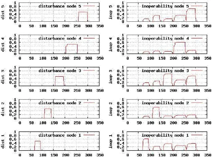
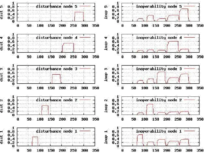
The result of the computation is presented to the user in the form of 2N plots showing the disturbance applied to the nodes and node's inoperability.
D 2.2.5 Provision of Prototype “Leontief-Based Tool” 17
Figure 2. Results of the inoperability dynamics for a system of 5 nodes subject to disturbance.
As an example Figure 2 presents a simulation done on a system of 5 nodes, disturbance plots are on the left-hand side, inoperability is on the right.
As can be seen in Figure 2 the disturbances applied to the nodes are not fixed in time. This is because the LBS operates as a controller, that is, in an endless loop it reads the networks state allowing to change the disturbance in “real time”. In other words, it is possible to introduce new disturbances and to eliminate, increase or decrease existing disturbances at any given moment of the simulation.
2.3.4 Optimisation
While the first LBS dynamics feature gives the user the possibility to gain some intuition of how networks react to a disturbance coming from other networks or, in other words, how inoperability spreads over a network of networks, the second feature suggests a way to control that reaction by increasing the inoperability of a single network (system's node) artificially. As in case of a cascade in an electrical grid, a controlled increase of inoperability of one part of the system (e.g., a shut down of a line such that a whole area gets disconnected) can prevent the cascade from reaching other areas and, thus, the total damage decreases. Therefore, the goal is to increase the inoperability of a node in order to prevent the disturbance from propagating to the other nodes, thus, decreasing the total inoperability. For this aim an objective function, which represents a measure of the total inoperability, should be defined and then minimized. “Total inoperability” is the inoperability of the network of networks, which the LBS system stands for. To implement this strategy two additional elements are introduced to the system: a sink node (denoted as node zero), representing any external demand, and nodes’ buffers. The buffers function as a “store house” of the nodes.
D 2.2.5 Provision of Prototype “Leontief-Based Tool” 18
Let node i produce for node j an amount wij of its product. If, for reason of disturbance, node j is unable to collect the product, then node i simply puts it in its buffer to be used once node j is again operable. If now for some reason node i has a reduction in its operability that is a decrease in its production, it can compensate this decrease “taking” what is stored in the buffer. This behaviour of the buffers can be described as:
( ) ( ) ( )
∑
( )
= + − = + n j ij ij i i i t b t x t x t b 0 1 ρ (6)where xij(t) is the inoperability between networks (nodes) i and j, that is the relative amount of product not delivered to j from i at time t:
( )
( )
ij ij ij ij W t w W t x = − (7)Wij is what should be produced and wij(t) < Wij is the amount produced at time t.
In [Tron06], the relation between system productivity and system inoperability is used to formulate the problem of minimizing the total inoperability as a Mixed Integer Linear Problem (MILP). The objective function to minimize is:
⎟ ⎠ ⎞ ⎜ ⎝ ⎛ +
∑
∑
∑
= = − = n i n i t i i t i i h t t x y 1 1 , , 1 0 θ μ γ (8)where yi,t = xi0(t) denotes the inoperability of the networks (nodes) versus the external demand represented as the sink node (node zero)
and
μi defines how important is to us subsystem i with respect to all others subsystems in the network;
θi defines how important is to us the output of subsystem i with respect to all other subsystem outputs;
γt defines the importance in our planning horizon h of the overall system inoperability at time t defined by expression (8).
Given a network and initial inoperability settings of all nodes, the LBS tool computes new inoperability settings, so as to minimize the objective function defined above.
The optimisation simulation also works as a controller. That is, in an endless loop it reads the network state and computes the new settings for node inoperabilities on a given horizon. The outputs are: node's inoperability, node's external demand inoperability, buffer values and the objective function values.
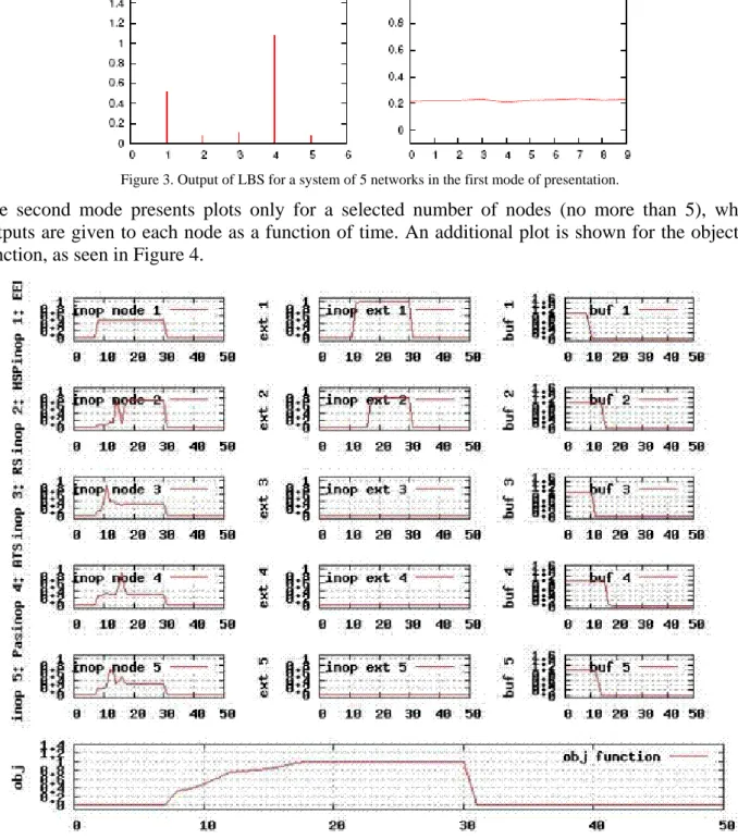
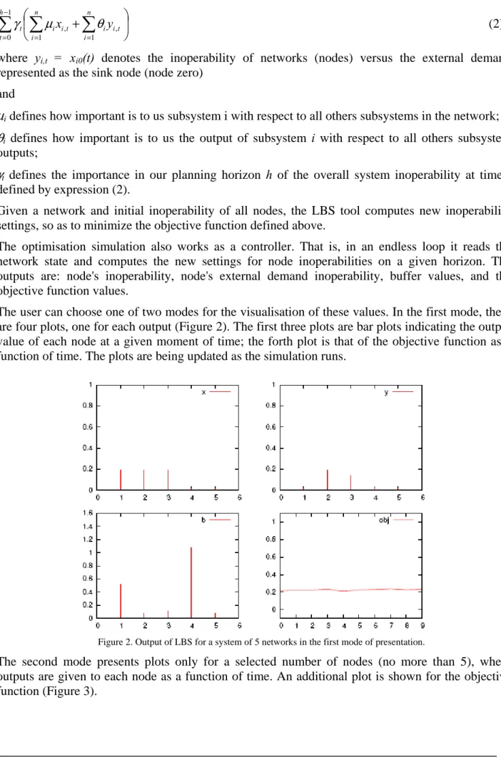
The user can choose one of two modes for the visualisation of these values. In the first mode, there are four plots one for each output, as can be seen in Figure 3. The first three plots are bar plots indicating the output value of each node at a given moment of time, the forth plot is that of the objective function as a function of time. The plots are being updated as the simulation runs.
D 2.2.5 Provision of Prototype “Leontief-Based Tool” 19
Figure 3. Output of LBS for a system of 5 networks in the first mode of presentation.
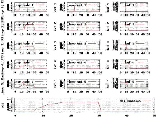
The second mode presents plots only for a selected number of nodes (no more than 5), where outputs are given to each node as a function of time. An additional plot is shown for the objective function, as seen in Figure 4.
D 2.2.5 Provision of Prototype “Leontief-Based Tool” 20
Figure 4 shows the output of LBS for a system of 5 networks in the second mode of presentation. Each column of plots contains 5 plots representing the 5 networks of the system. The three columns from left to right are the measures of inoperability, external inoperability and buffer contents. At the bottom are the objective function values during the 50 time steps of the simulation.
3.
Introduction to the Leontief-Based Simulation (LBS) Tool
3.1
Home page
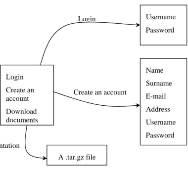
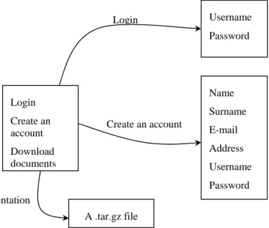
Figure 5. Organization of the Home page
The Home page of the Leontief-Based Simulation Tool is the entrance to the simulator. Its Web address is http://ciip.casaccia.enea.it/leontief. From this page the user can (Figure 5):
• Login to the tool,
• Download documentation, • Create a Leontief account.
3.2
Creating an account to the tool
In order to create an account, the user has to fill in some obligatory fields: name, surname, an e-mail address, username, and password. That information is necessary for the administration of the tool.
3.3
Downloading documentation
The user can download the documentation of the tool in .tar.gz format. The zipped file contains a brief tutorial of how to create the input files, a technical report describing the tool and the input files used in the technical report.
3.4
User login to the Leontief-based tool
The login to the LBS tool is made via user name and password.
3.5
Managing a Leontief account
From the page of management (Figure 6) the user can run the Leontief algorithm selecting the maximum execution time in seconds or minutes.
Login Create an account Download documents Username Password Login Name Surname E-mail Address Username Password Create an account A .tar.gz file Documentation
D 2.2.5 Provision of Prototype “Leontief-Based Tool” 21
Figure 6. Management of the network
Before the execution the following actions can be done: • creating a network with maximum 5 nodes,
• uploading the network giving the respective files size.dat, rho.dat, inop.dat, fail.dat, and beta.dat,
• or executing the network that is already created during the last user’s access to the site (download the network).
From this page the user can start or stop the execution. 3.5.1 Executing the algorithm
If the user chose to start the execution of the Leontief algorithm, a new window opens showing the diagrams of inoperability and disturbance of the network nodes at run time.
The diagrams for the five network nodes (subnetworks) are shown in two columns. The first column displays the disturbance for every node of the network as a function of time. The second column depicts nodes’ inoperability as a function of time.
The algorithm’s execution can be stopped at any time. At the end of the execution the diagrams (the plots) can be saved (downloaded) for future use and examination. They are displayed as a JPEG file. Create a network Upload a network Download the network Run the network Number of nodes Size.dat Leontief technical coefficients Rho.dat Inoperability values Inop.dat Sensibility to failure Beta.dat Disturbance values Fail.dat Number of nodes Size.dat Leontief technical coefficients Rho.dat Inoperability values Inop.dat Sensibility to failure Beta.dat Disturbance values Fail.dat Number of nodes n Leontief technical coefficients ρij Inoperability values xij Sensibility to failure γi Disturbance values di New network Upload Download Diagrams
D 2.2.5 Provision of Prototype “Leontief-Based Tool” 22
3.5.2 Creation of a network
To create a new network the user can select the option “Create a Network” in the main menu. He/she can select up to five nodes (subnetworks) for the network.
Then he/she is prompted to insert the Leontief technical coefficients, ρij, for the network arcs in a table. A file rho.dat is created that contains the coefficients chosen.
The creation of the network continues with the insertion of the inoperability values, xij, for the network nodes. A file inop.dat is created with the values chosen.
In the next window, the values of the failure sensibility of the nodes, γi, are inserted. A file beta.dat is created.
The disturbance values, di, for the network nodes are inserted in the next window. A file fail.dat is created.
In that way, the network is created and the user can proceed with its execution. 3.5.3 Downloading the network
From the main menu the user can download the network that is present in the account for future use and experimentation. The following files are downloaded: rho.dat, size.dat, beta.dat, fail.dat, and inop.dat. If the user follows the links to the files, he/she can see the values of the parameters inserted.
3.5.4 Uploading the network
If the user wants to use a network that is already created during the previous access of the user to the modelling tool, he/she can upload the files rho.dat, size.dat, beta.dat, fail.dat, and inop.dat. 3.5.5 Starting the execution
There are three options for the user before he/she starts the execution of the model:
• If no network is specified, the LBS tool starts to execute the network from the last user’s access to the tool.
• If the user wants to create a new network, after he/she inserts the input parameters, the LBS tool executes the network just created.
• If the user has uploaded a network of his/her choice, then the LBS tool executes that network. 3.5.6 Stopping the execution
The execution of the model can be stopped at any point.
For a detailed description of the Leontief-based tool see Appendix A.
4.
References
[NAT] http://irriis.nat.ylichron.it/default.aspx?fl=0
[Starlink] http://www.starlink.rl.ac.uk/star/docs/sun33.htx/sun33.html
[Leontief] http://ciip.casaccia.enea.it/leontief or http://leontief.casaccia.enea.it/Leontief/.
[HaJi01] Pu Jiang and Y. Y. Haimes, “Risk Management for Leontief-Based Interdependent Systems”, Risk Analysis, Vol. 24, No. 5, 2004
[Seto07] R. Setola and S. De Porcellinis, “A Methodology to Estimate Input-Output Inoperability Model Parameters”
D 2.2.5 Provision of Prototype “Leontief-Based Tool” 23
[Tron06] E. Tronci, “Methods and Instruments for Evaluation of Interdependencies among Technological Networks and Minimization of Inoperability Caused by Natural and/or Deliberate Events”, Technical Report, Nov. 2006
[Rosa08] V.Rosato et al., “Is the topology of the Internet network really fit to sustain its function?”, Physica A 387 (2008), pp. 1689-1704.
D 2.2.5 Provision of Prototype “Leontief-Based Tool” 24
Appendix A
Leontief-Based Simulation Tool
User’s Guide
1. The Leontief-based simulation tool: the algorithm
1.1 Inoperability dynamics of interdependent networks
The Leontief-Based Simulation (LBS) tool [Leontief] simulates a system composed of a set of interconnected networks (a network of networks). It allows the evaluation of the impact a fault in one network has on the rest of the system in terms of networks' inoperability. The basic assumption of this approach is that each network produces some product or gives some service. The interdependency is introduced by the fact that the products/services of one network are consumed by other network/s.
1.2 The system
The LBS system can be formulated as follows:
Consider a system S = {1, …, n} consisting of n interdependent subsystems. Each subsystem is also called a node of S. If node i sends a product or gives some service to node j, there is an edge from node i to node j. The edge's magnitude implies the strength of the dependency between each two nodes of the system i, j ∈ S. It is denoted as ρij and is assumed to be constant in time, ρij∈
[ ]
0,1. The matrix of the dependencies is denoted as ρ and ρij are also referred to as the Leontief technical coefficients. It is further assumed that each of the nodes is characterized by its inoperability denoted as xi. A node i is said to be fully operable, if xi = 0, and non operable, if xi = 1.In a normal situation, i.e., when no disturbance is introduced to the system, all subsystems are assumed to be fully operable, hence xi = 0 ∀ i ∈ S. To estimate the impact of a disturbance in one or more of the nodes the following inoperability dynamics equation is introduced [Tron06]:
( )
( )
( )
⎭ ⎬ ⎫ ⎩ ⎨ ⎧ + = +∑
= n j ij j i i i t x t d t x 1 , 1 min 1 ρ γ (1)where ρ is the Leontief coefficients matrix, di(t) ∈ [0, 1] is the disturbance (fault injection) at node i and γi is the sensibility of node i to faults.
1.3 The simulation
Given a set S of nodes and their initial inoperability xi(t=t0) the LBS tool computes the inoperability of all nodes for t > t0 according to equation (1).
The result of the computation is presented to the user in the form of 2N plots showing the disturbance applied to the nodes and node's inoperability.
As an example Figure 1 presents a simulation done on a system of 5 nodes, disturbance plots are on the left-hand side, inoperability is on the right.
D 2.2.5 Provision of Prototype “Leontief-Based Tool” 25
As can be seen in Figure 1 the disturbances applied to the nodes are not fixed in time. This is because the LBS tool operates as a controller, that is, in an endless loop it reads the networks’ state, allowing change of the disturbance in “real time”. In other words, it is possible to introduce new disturbances and to eliminate, increase or decrease existing disturbances at any given moment of the simulation.
Figure 1. Results of the inoperability dynamics for a system of 5 nodes subject to disturbance.
1.4 Optimisation
While the first LBS dynamics feature gives the user the possibility to gain some intuition of how networks react to a disturbance coming from other networks or, in other words, how inoperability spreads over a network of networks, the second feature suggests a way to control that reaction by increasing the inoperability of a single network artificially. For example, in case of a cascade in an electrical grid, a controlled increase of inoperability of one part of the system (such as a shut down of a line to disconnect the whole area) can prevent the cascade from reaching other areas and, thus, the total damage decreases. The goal is to increase the inoperability of a node in order to prevent the disturbance from propagating to the other nodes, thus, decreasing the total inoperability. For this aim an objective function, which represents a measure of the total inoperability, should be defined and then minimized. By “total inoperability” we mean the inoperability of the network of networks, which the LBS system stands for. To implement this strategy two additional elements are introduced to the system: a sink node (denoted as node zero), representing any external demand, and nodes’ buffers. The buffers function as a “store house” of the nodes.
D 2.2.5 Provision of Prototype “Leontief-Based Tool” 26
⎟ ⎠ ⎞ ⎜ ⎝ ⎛ +
∑
∑
∑
= = − = n i n i t i i t i i h t t x y 1 1 , , 1 0 θ μ γ (2)where yi,t = xi0(t) denotes the inoperability of networks (nodes) versus the external demand represented as the sink node (node zero)
and
μi defines how important is to us subsystem i with respect to all others subsystems in the network;
θi defines how important is to us the output of subsystem i with respect to all others subsystem outputs;
γt defines the importance in our planning horizon h of the overall system inoperability at time t defined by expression (2).
Given a network and initial inoperability of all nodes, the LBS tool computes new inoperability settings, so as to minimize the objective function defined above.
The optimisation simulation also works as a controller. That is, in an endless loop it reads the network state and computes the new settings for node inoperabilities on a given horizon. The outputs are: node's inoperability, node's external demand inoperability, buffer values, and the objective function values.
The user can choose one of two modes for the visualisation of these values. In the first mode, there are four plots, one for each output (Figure 2). The first three plots are bar plots indicating the output value of each node at a given moment of time; the forth plot is that of the objective function as a function of time. The plots are being updated as the simulation runs.
Figure 2. Output of LBS for a system of 5 networks in the first mode of presentation.
The second mode presents plots only for a selected number of nodes (no more than 5), where outputs are given to each node as a function of time. An additional plot is shown for the objective function (Figure 3).
D 2.2.5 Provision of Prototype “Leontief-Based Tool” 27
Figure 3. Output of LBS for a system of 5 networks in the second mode of presentation.
Figure 3 shows the output of the LBS tool for a system of 5 networks in the second mode of presentation. Each column of plots contains 5 plots representing the 5 networks of the system. The three columns from left to right are the measures of inoperability, external inoperability and buffer contents. At the bottom are the objective function values during the 50 time steps of the simulation.
2. Introduction to the Leontief-Based Simulation (LBS) Tool: The User
Prospective
2.1 Home page
The Home page of the Leontief-Based Simulation Tool is the entrance to the simulator. Its Web address is http://ciip.casaccia.enea.it/leontief. From this page the user can (Figure 4):
• Login to the tool,
• Download documentation, • Create a Leontief account.
D 2.2.5 Provision of Prototype “Leontief-Based Tool” 28
Figure 4. Organisation of the Home page
Figure 5. The Leontief-Based Simulator Home page.
Login Create an account Download documents Username Password Login Name Surname E-mail Address Username Password Create an account A .tar.gz file Documentation
D 2.2.5 Provision of Prototype “Leontief-Based Tool” 29
2.2 Creating an account to the tool
In order to create an account (Figure 6), the user has to fill in some obligatory fields: name, surname, an e-mail address, username, and password. That information is necessary for the administration of the tool.
Figure 6. Creating an account
2.3 Downloading documentation
The user can download the documentation of the tool in .tar.gz format. The zipped file contains a brief tutorial of how to create the input files, a technical report describing the tool and the input files used in the technical report.
2.4 User login to the Leontief-based tool
The login to the LBS tool is made via user name and password.
2.5 Managing a Leontief account
From the page of management (Figure 8) the user can run the Leontief algorithm selecting the maximum execution time in seconds or minutes. Before the execution the following actions can be done (Figure 7):
• creating a network with maximum 5 nodes,
• uploading the network giving the respective files size.dat, rho.dat, inop.dat, fail.dat, and beta.dat,
D 2.2.5 Provision of Prototype “Leontief-Based Tool” 30
• or executing the network that is already created during the last user’s access to the site (download the network).
From this page the user can start or stop the execution.
Figure 7. Management of the network
Create a network Upload a network Download the network Run the network Number of nodes Size.dat Leontief technical coefficients Rho.dat Inoperability values Inop.dat Sensibility to failure Beta.dat Disturbance values Fail.dat Number of nodes Size.dat Leontief technical coefficients Rho.dat Inoperability values Inop.dat Sensibility to failure Beta.dat Disturbance values Fail.dat Number of nodes n Leontief technical coefficients ρij Inoperability values xij Sensibility to failure γi Disturbance values di New network Upload Download Diagrams
D 2.2.5 Provision of Prototype “Leontief-Based Tool” 31
Figure 8. The Management page 2.5.1 Executing the algorithm
If the user chose to start the execution of the Leontief algorithm, a new window opens showing the diagrams of inoperability and disturbance of the network nodes at run time (Figure 9).
The diagrams for the five network nodes (subnetworks) are shown in two columns. The first column displays the disturbance for every node of the network as a function of time. The second column depicts nodes’ inoperability as a function of time.
The algorithm’s execution can be stopped at any time. At the end of the execution the diagrams (the plots) can be saved (downloaded) for future use and examination. They are displayed as a JPEG file.
D 2.2.5 Provision of Prototype “Leontief-Based Tool” 32
Figure 9. Executing the algorithm 2.5.2 Creation of a network
To create a new network the user can select the option “Create a Network” in the main menu. He/she can select up to five nodes (subnetworks) for the network.
D 2.2.5 Provision of Prototype “Leontief-Based Tool” 33
Then he/she is prompted to insert the Leontief technical coefficients, ρij, for the network arcs in a table. A file rho.dat is created that contains the coefficients chosen.
The creation of the network continues with the insertion of the inoperability values, xij, for the network nodes. A file inop.dat is created with the values chosen.
In the next window, the values of the failure sensibility of the nodes, γi, are inserted. A file beta.dat is created.
The disturbance values, di, for the network nodes are inserted in the next window. A file fail.dat is created.
In that way, the network is created and the user can proceed with its execution.
2.5.3 Downloading the network
From the main menu the user can download the network that is present in the account for future use and experimentation (Figure 10). The following files are downloaded: rho.dat, size.dat, beta.dat, fail.dat, and inop.dat. If the user follows the links to the files, he/she can see the values of the parameters inserted.
Figure 10. Downloading the network 2.5.4 Uploading the network
If the user wants to use a network that is already created during the previous access of the user to the modelling tool, he/she can upload the files rho.dat, size.dat, beta.dat, fail.dat, and inop.dat (Figure 11).
D 2.2.5 Provision of Prototype “Leontief-Based Tool” 34
Figure 11. Uploading a network 2.5.5 Starting the execution
There are three options for the user before he/she starts the execution of the model:
• If no network is specified, the LBS tool starts to execute the network from the last user’s access to the tool.
• If the user wants to create a new network, after he/she inserts the input parameters, the LBS tool executes the network just created.
• If the user has uploaded a network of his/her choice, then the LBS tool executes that network.
2.5.6 Stopping the execution
The execution of the model can be stopped at any point.
2.6 Some examples
Scenario 1:
We consider a network with five nodes representing five infrastructures (Figure 12). The example is taken from [Bald05]. The five infrastructures are: electrical energy provider (denoted with 1 in Figure 12), hospital service system (node 2 in Figure 12), railway system (node 3 in Figure 12), alternative transport system (node 4 in Figure 12), and passengers (node 5 in Figure 12).
D 2.2.5 Provision of Prototype “Leontief-Based Tool” 35
Figure 12. Network with five nodes.
The values of ρij are (as in [Tron06]):
0 . 0 5 . 0 0 . 0 2 . 0 0 . 0 0 . 0 0 . 0 1 . 0 0 . 0 5 . 0 5 . 0 0 . 0 0 . 0 2 . 0 1 . 0 1 . 0 0 . 0 0 . 0 0 . 0 1 . 0 1 . 0 1 . 0 5 . 0 1 . 0 0 . 0
The initial inoperabilities, xi, are all 0.0, i.e., all nodes are operable. The sensitivity to faults, γi, is: 0.1; 0.4; 0.0; 0.0; 0.0. The disturbance, di, is: 0.5; 0.0; 0.0; 0.0; 0.0. The model is run for 60 sec.
Figure 13. Disturbance at node 1 (electrical grid) and its influence on the system
5 2
4
D 2.2.5 Provision of Prototype “Leontief-Based Tool” 36
Scenario 2
A network with three nodes. The Leontief technical coefficients are:
17 . 0 27 . 0 37 . 0 55 . 0 25 . 0 15 . 0 3 . 0 4 . 0 0 . 0
Initial inoperability: 0.1; 0.2; 0.3. Disturbance: 0.9; 0.2; 0.0. Sensitivity to fault: 0.05; 0.9; 0.0. Execution time: 30 sec.
Figure 14. Disturbance and inoperability of a network with 3 nodes.
3. Comments and Concluding Remarks
The Leontief-based simulation tool is still in process of development. Both the underlying algorithm and the tool have to be elaborated in order to obtain satisfying results. From the user prospective, the fact that the tool is Web-based facilitates its use. The user has the opportunity to upload a network and analyze it under different conditions. The disturbance values can be changed to investigate different scenarios.
The optimization of the algorithm aims at minimizing the objective function of total inoperability. That part of the simulation is available only under Linux and is not Web-based yet. A user-friendly interface has to be designed to make the analysis easy to carry out.
There are also many interesting questions to be answered about the algorithms and methods to study interdependencies of critical infrastructures:
D 2.2.5 Provision of Prototype “Leontief-Based Tool” 37
• To obtain more realistic data about the interdependencies – Leontief technical coefficients. • To study if these coefficients are a function of time; to see the process.
• To apply different disturbances.
• To study different scenarios of optimisation.
References
[Tron06] E. Tronci, “Methods and Instruments for Evaluation of Interdependencies among Technological Networks and Minimization of Inoperability Caused by Natural and/or Deliberate Events”, Technical report, Nov. 2006
[Leontief] http://ciip.casaccia.enea.it/leontief or http://leontief.casaccia.enea.it/Leontief/
[Bald05] C. Balducelli, S. Bologna, A. Di Pietro, and G, Vicoli, “Analysing Interdependecies of Critical Infrastructures Using Agent Discrete-Event Simulation”, Int. Journal of Emergency Management, 2005.