Gemini Observations of Galaxies in Rich Early Environments (GOGREEN) I: survey description

Gemini Observations of Galaxies in Rich Early Environments

(GOGREEN) I: survey description

Michael L. Balogh,

David G. Gilbank,

Adam Muzzin,

Gregory Rudnick,

Michael C. Cooper,

Chris Lidman,

Andrea Biviano,

Ricardo Demarco,

Sean L. McGee,

Julie B. Nantais,

Allison Noble,

Lyndsay Old,

Gillian Wilson,

Howard K. C. Yee,

Callum Bellhouse,

Pierluigi Cerulo,

Jeffrey Chan,

Irene Pintos-Castro,

Rane Simpson,

Remco F. J. van der Burg,

Dennis Zaritsky,

Felicia Ziparo,

Mar´ıa Victoria Alonso,

Richard G. Bower,

Gabriella De Lucia,

Alexis Finoguenov,

Diego Garcia Lambas,

Hernan Muriel,

Laura C. Parker,

Alessandro Rettura,

Carlos Valotto

and Andrew Wetzel

†

Affiliations are listed at the end of the paper

Accepted 2017 May 31. Received 2017 May 29; in original form 2017 May 3

A B S T R A C T

We describe a new Large Program in progress on the Gemini North and South telescopes: Gemini Observations of Galaxies in Rich Early Environments (GOGREEN). This is an imaging

and deep spectroscopic survey of 21 galaxy systems at 1<z<1.5, selected to span a factor

>10 in halo mass. The scientific objectives include measuring the role of environment in the

evolution of low-mass galaxies, and measuring the dynamics and stellar contents of their host haloes. The targets are selected from the SpARCS, SPT, COSMOS, and SXDS surveys, to be the evolutionary counterparts of today’s clusters and groups. The new red-sensitive Hamamatsu detectors on GMOS, coupled with the nod-and-shuffle sky subtraction, allow simultaneous

wavelength coverage overλ∼0.6–1.05µm, and this enables a homogeneous and statistically

complete redshift survey of galaxies of all types. The spectroscopic sample targets galaxies

with AB magnitudesz<24.25 and [3.6]µm<22.5, and is therefore statistically complete for

stellar massesM_∗1010.3_{M, for all galaxy types and over the entire redshift range. Deep,}

multiwavelength imaging has been acquired over larger fields for most systems, spanningu

throughK, in addition to deep IRAC imaging at 3.6µm. The spectroscopy is∼50 per cent

complete as of semester 17A, and we anticipate a final sample of∼500 new cluster members.

Combined with existing spectroscopy on the brighter galaxies from GCLASS, SPT, and other sources, GOGREEN will be a large legacy cluster and field galaxy sample at this redshift that spectroscopically covers a wide range in stellar mass, halo mass, and clustercentric radius. Key words: galaxies: clusters: general – galaxies: evolution.

1 I N T R O D U C T I O N

Galaxy clusters are extraordinarily valuable as laboratories for a wide range of tests and experiments. They play a central role in studies of cosmology (e.g. Carlberg et al. 1996; Wang & Stein-hardt 1998; Haiman, Mohr & Holder2001; Sehgal et al.2011;

_{E-mail:mbalogh@uwaterloo.ca} †Caltech-Carnegie Fellow.

Benson et al.2013), galaxy and structure formation (e.g. Dressler 1980; Butcher & Oemler1984; Balogh et al.1999b; Ellingson et al. 2001; van den Bosch et al.2008; Peng et al.2012; Wetzel et al. 2013), high-energy physics (e.g. Mohr, Mathiesen & Evrard1999; Tozzi & Norman2001; Pfrommer & Enßlin2004; Bialek, Evrard & Mohr2001; Balogh, Babul & Patton1999a; Cavagnolo et al. 2008; Fabian et al. 2000; Aharonian et al.2017), supermassive black hole growth (e.g. McNamara & Nulsen2007; Alexander & Hickox2012), and for the determination of the nature of dark matter (e.g. Clowe et al.2006; Randall et al.2008; Bradaˇc et al.2008; Jee

C

et al.2012). Their enormous gravitational potentials allow them to act as cosmic ‘calorimeters’, maintaining an observable record of all the energy inputs and outputs associated with galaxy formation over the history of the Universe (e.g. Voit & Bryan2001; Gon-zalez, Zaritsky & Zabludoff2007; Balogh et al.2008; Vikhlinin et al.2006; Puchwein, Sijacki & Springel 2008). They host the most massive galaxies, whose stars are among the first to form (e.g. Lidman et al.2012; Lin et al.2013; Marchesini et al.2014; Fassbender et al.2014). Clusters are also the ideal places to study rare and extraordinary perturbations to galaxy evolution, such as hydrodynamic stripping of gas (e.g. Vollmer et al.2000; Merluzzi et al.2013; Boselli et al.2016), tidal stripping of matter (Natara-jan, Kneib & Smail2002), and high-speed gravitational encounters. Much of what we have learned about galaxy evolution is thanks to years of research on these systems.

Atz>1, when the gas accretion rates, relative gas masses, and star formation rates (SFRs) of galaxies were much higher than they are today, the interactions between galaxies and their environments are also expected to be very different. Large spectroscopic samples have now been built up in clusters approachingz∼1 (Muzzin et al. 2012; Balogh et al.2014; Bayliss et al.2016), but little is known about the physical properties of typical galaxies inz>1 clusters. Those spectroscopic studies that do exist are generally restricted to the most massive galaxies (e.g. Snyder et al.2012; Lotz et al.2013) or emission-line galaxies (e.g. Zeimann et al.2013; Nanayakkara et al.2016) in the most massive clusters (e.g. Nantais et al.2013; Martini et al.2013; Stanford et al.2014). Studying the faint, and more common, galaxy population at 1< z < 1.5 usually relies heavily on photometric redshifts (e.g. Nantais et al.2016).

Thus for the first round of Gemini Large and Long Programs in 2014, we proposed an ambitious distant cluster legacy survey, titledGemini Observations of Galaxies in Rich Early ENvironments (GOGREEN), using the GMOS instruments on the North and South telescopes. GMOS has several capabilities that make it ideally suited to studies of galaxy clusters atz∼1. The nod-and-shuffle (n&s) mode (Glazebrook & Bland-Hawthorn2001) allows excellent sky subtraction at red wavelengths, resulting in much greater efficiency for faint galaxies (as exploited by the GDDS1_{; Abraham et al.2004).}

Moreover, the n&s microslits are up to three times smaller than normal slits, allowing them to be placed with a very high surface density. Together with the new Hamamatsu detectors, which have good sensitivity up toλ∼1.05µm, GMOS spectroscopy of faint objects is now feasible at 1.0<z<1.5.

The objective of the survey is to build directly on the work we have done with Gemini in constructing the GCLASS2

clus-ter (Muzzin et al.2012) and GEEC23_{group (Balogh et al.2014)}

surveys. GCLASS was a GMOS survey consisting of∼450 spectro-scopically confirmed members of 10 massive clusters at 0.86<z<

1.34. Among other things, this enabled new insight into the environ-mental transformation of galaxies (Muzzin et al.2014; Foltz et al. 2015; Noble et al.2013,2016), the stellar mass content and distri-bution in clusters (van der Burg et al.2013,2014), cluster dynamics (Biviano et al.2016), and growth of the brightest cluster galaxies (Lidman et al.2012). An independent but highly complementary survey was GEEC2, which used a sample of 10 X-ray-detected groups in the COSMOS field to address similar questions of galaxy evolution (Balogh et al.2011; Mok et al.2013,2014) and group

1_{Gemini Deep Deep Survey.}

2_{Gemini CLuster Astrophysics Spectroscopic Survey.} 3_{Galaxy Environment Evolution Collaboration 2.}

dynamics (Hou et al. 2013). The combination of GEEC2 and GCLASS provides a sample that spans more than two orders of magnitude in halo mass, allowing the measurement of halo mass effects on the environmental quenching measurement (Balogh et al. 2016).

GOGREEN uses a similar strategy to extend these works to 1.0

<z<1.5 with comparably dense spectroscopy on 21 systems span-ning a wide range in halo mass. An important feature of GOGREEN is that our systems are chosen to be representative of the progeni-tors of today’s clusters; this is complementary to efforts focused on the most massive clusters at high redshift, which have few, if any, local descendants. The survey will obtain spectroscopy on a large sample of very faint targets,z<24.25 and [3.6]<22.5 to obtain a sample of confirmed cluster members, measure cluster dynam-ics and galaxy stellar populations, and provide critical calibration of photometric redshifts. The survey design is driven by three key science goals, and an aim to provide a legacy data set that is useful to the broader community. These goals are described in more detail below.

1.1 Environmental quenching and growth of the stellar mass function

Despite a solid theoretical foundation for the gravitational growth of dark matter structure, galaxy formation models have great dif-ficulty simultaneously reproducing the rate of decline in global SFR, the mass dependence of this decline, and the star formation histories of satellite galaxies (Bower, Benson & Crain2012; Wein-mann et al.2012; Hirschmann et al.2014; De Lucia et al.2012; Henriques et al.2015; Genel et al.2014; Trayford et al.2015). These problems may be related, as they are all sensitive to assumptions about how gas accretion, ejection and heating processes depend on epoch, environment, and halo mass (McGee, Bower & Balogh 2014). The conventional picture of the interaction between galax-ies and their surroundings is that galaxgalax-ies enter dense environments with a reservoir of gas (either in the stellar disc, or the halo), and that star formation declines as this reservoir is removed (e.g. Balogh, Navarro & Morris2000; Bower et al.2006; Schawinski et al.2014; Fillingham et al.2015). However, cosmological simulations show that galaxies grow as a result of continuous infall from surrounding filaments (e.g. Kereˇs et al.2005), a scenario that is supported by in-direct observational arguments (e.g. Dav´e, Finlator & Oppenheimer 2012; Lilly et al.2013). While a reservoir may play a role at low redshift, at higher redshift the supply of fresh gas fully dominates over the consumption of the reservoir. This change leads to a predic-tion that dense environments shut down star formapredic-tion even more rapidly atz>1 than at low redshift (McGee et al.2014; Balogh et al.2016; van de Voort et al.2017). The sensitivity of the observed galaxy population to gas accretion and outflow rates on large scales allows us to use trends with environment to put constraints on feed-back and accretion models that may be relevant to the evolution of all galaxies.

Simple but powerful indicators of SFR suppression (or ‘quench-ing’) are the evolution of the quiescent galaxy stellar mass function, and the stellar mass dependence of the quiescent fraction (e.g. van den Bosch et al.2008; Peng et al.2010; Fillingham et al.2016; Balogh et al.2016). From these measurements alone, it is possi-ble to put strong constraints on the quenching time-scale and its evolution (e.g. Tinker & Wetzel2010), which is a powerful indica-tor of how gas-supply and removal mechanisms change with time (McGee et al.2014; Balogh et al.2016; Fossati et al.2017). In the field population, the quiescent galaxy mass function evolves rapidly,

as star formation is shut down first in the most massive galaxies, and later in dwarfs (e.g. Muzzin et al.2013a). In massive clusters, this is clearly seen as the growth of the ‘red sequence’ (e.g. De Lucia et al.2004; Tanaka et al.2005; Gilbank & Balogh2008; Rudnick et al.2009,2012). Atz<1, most models predict many more low-mass, quiescent galaxies than are observed, a consequence of the well-established overquenching problem (Weinmann et al.2011; Hirschmann et al. 2014; De Lucia et al. 2012; Henriques et al. 2015; Genel et al.2014; Trayford et al.2015).

The situation is much less clear at higher redshift (e.g. Nantais et al.2016), where the gas content, accretion rates, and SFRs of galaxies are so much higher, and even galaxies in cluster cores have only been satellites for a few Gyr. Moreover, the higher average SFR of field galaxies, and the increased rate at which they are ac-creted by the cluster, translates directly into a much higher fraction of galaxies observed in the ‘transition phase’ between actively star forming and quiescent (Poggianti et al.2009; Mok et al.2014). Ex-ceptional sensitivity to the galaxy transformation time-scale can be obtained from fairly straightforward modelling of the radial gradi-ents and projected phase space distribution of such subpopulations, compared with the quiescent and star-forming galaxies (e.g. Balogh et al.2000; Ellingson et al.2001; McGee et al.2009; Noble et al. 2013; Taranu et al.2014; Muzzin et al.2014; Haines et al.2015).

GOGREEN is designed specifically to measure the quiescent fraction of galaxies at 1.0< z<1.5, over a factor>10 in halo mass, with a spectroscopic sample statistically complete for all galaxy types down to stellar masses ofM_∗∼1010.3_M

. In addi-tion to the targeted clusters and groups, the survey will result in a comparably-sized field sample selected in the same way. The deep, multiwavelength imaging ensures a robust and homogeneous sep-aration of passive from star-forming galaxies, and a photometric redshift catalogue that is essential to account for the spatial incom-pleteness of the spectroscopic sample. When complete, the total spectroscopic sample size, including bright galaxy spectroscopy from GCLASS and other published catalogues, will be comprised of∼1000 cluster members; about half of these will be newly ac-quired via GOGREEN. This will ensure that statistical uncertain-ties on the quenched fraction, in bins of stellar and halo mass, are small enough to distinguish between different physical models as described in Balogh et al. (2016).

1.2 The hierarchical assembly of baryons

It is a fundamental prediction ofcold dark matter (CDM) theory that massive clusters are built from haloes of lower mass: groups and isolated galaxies (e.g. Berrier et al.2009; De Lucia et al.2012; Bullock, Kravtsov & Weinberg2001). Since it is difficult to pref-erentially remove stars from dark matter dominated systems, when these systems merge the fraction of total mass in stars can only increase (via star formation) or remain constant. Therefore, mea-surement of the stellar fraction, gas fraction, and SFR in haloes of a given mass provide one of the closest possible links between galaxies and this basic prediction of theCDM theoretical frame-work (Kravtsov, Nagai & Vikhlinin2005; Gonzalez, Zaritsky & Zabludoff2007; Balogh et al.2008; Giodini et al.2009; Gonzalez et al.2013; Leauthaud et al.2011,2012). Precision measurements of this type are essential for calibrating and constraining models, and are an essential complement to abundance-matching or halo occupation distribution model approaches (e.g. Behroozi, Wechsler & Conroy2013).

With GOGREEN, we will directly measure the central and total stellar mass of haloes at 1.0<z<1.5. The spatial and

dynami-cal distribution of cluster galaxies is sensitive not only to the field accretion rate, but also to the dynamical friction time and galaxy merger and disruption time-scales. These rates are not well under-stood theoretically (e.g. De Lucia et al.2010), despite being primar-ily gravitational processes, and observations of these distributions provide valuable constraints, as we have shown with GCLASS (e.g. van der Burg et al.2014).

1.3 Cluster dynamics and halo masses

At low redshift, the total mass content and distribution of galaxy clusters can be estimated by gravitational lensing, from the proper-ties of the intracluster plasma under the assumption of hydrostatic equilibrium, or from the distribution and kinematics of cluster galax-ies. The latter method always provides critical independent infor-mation from the other two, and is especially important for clusters at high redshifts, which are notoriously difficult to detect by their X-ray emission or weak-lensing signal. Atz>1.0, our knowledge of the mass profiles of galaxy clusters is therefore limited to only a few individual clusters.

Dynamical analyses of nearby clusters have shown theirM(r) to be well characterized by either an NFW (Navarro, Frenk & White 1997) or an Einasto, Kaasik & Saar (1974) profile, passive galaxy orbits to be isotropic and star-forming galaxy orbits to be radially elongated (e.g. Biviano & Girardi2003; Biviano & Katgert2004). The NFW and Einasto models appear to also fit well theM(r) of

z∼0.6 clusters, but the orbits of passive galaxies evolve withz, and atz∼0.6 are more similar to those of star-forming galaxies (Biviano & Poggianti2009; Biviano et al.2013).

Using a stack of∼400 galaxies in 10 clusters of the GCLASS sample, Biviano et al. (2016) have shown that theM(r) ofz∼1 clusters is still well described by the NFW model, with a concen-tration as predicted by numerical simulations, and that the orbits of passive and star-forming cluster galaxies are indistinguishable and mildly radially elongated. With GOGREEN we will trace this evolution toz∼1.5. We will be able to measure whether the NFW and Einasto models remain valid representations of the clusterM(r), which is particularly interesting as the onset of dynamical equilib-rium in galaxy clusters is still a poorly understood process (e.g. Dehnen & McLaughlin 2005). Combined with the velocity anisotropy profile β(r), we can measure the more fundamental pseudo-phase space profile (Dehnen & McLaughlin2005; Lapi & Cavaliere2009). Evolution in this profile can distinguish between cluster assembly via fast, violent relaxation processes, and smooth accretion of matter from the field (Hansen et al.2009).

1.4 Legacy science

GOGREEN will provide deep, multiwavelength imaging, and spec-troscopy over 21 systems spanning a factor >10 in halo mass. Future surveys like eRosita, Euclid and LSST will find large sam-ples of high-redshift clusters. These surveys rely on spectroscopic studies to calibrate their observable quantitites in way that is nec-essary for cosmological applications. The depth and completeness of GOGREEN spectroscopy is a good complement to efforts like Bayliss et al. (2016) and Stanford et al. (2014), which aim to sparsely sample relatively massive galaxies in a much larger set of clusters. A byproduct of our survey will be a deep spectroscopic field survey of>600 galaxies at 1.0<z<1.5, with homogeneous and well-understood selection criteria. At present, none of the existing wide-field spectroscopic surveys have the red sensitivity to match GOGREEN depth at 1.3<z<1.5. Claims about evolution in the

stellar mass function and star formation history, for example are based on photometric redshifts, which are notoriously unreliable in regions of parameter space where spectroscopic calibration is unavailable. The GOGREEN field survey will be twice the size of GDDS (Abraham et al.2004), and 0.5 mag deeper, allowing an unparalleled spectroscopic measurement of the galaxy mass func-tion, separated by galaxy type. It will provide a crucial calibration sample for photometric redshifts out toz=1.5, needed by surveys like LSST and PanStarrs.

In this paper, we describe the survey design (Section 2), spectro-scopic observations (Section 3), and the current status of the project (Section 4). All magnitudes reported in this paper are on the AB system.

2 S U RV E Y D E S I G N

2.1 Objectives

GOGREEN is designed primarily to learn about the stellar popula-tions in galaxies that inhabit massive haloes,M5×1013_M

, at 1.0<z<1.5. To do this, it is essential to cover a large range in both stellar mass and halo mass. In particular, it is important to study low stellar mass galaxies, which are rarely quenched in the field population. At 1.0<z<1.5, such galaxies are faint and red, making it challenging to even obtain a redshift since most strong absorption features are redshifted to wavelengths where night sky emission lines are strong. To take advantage of the range in halo mass, it is important to be able to characterize those haloes, which, in part, requires redshifts for as many cluster members as possible, including the brightest ones. These two goals – very deep spec-troscopy of faint galaxies, together with a large number of redshifts for bright galaxies – are difficult to achieve, and most cluster sur-veys aim to do one or the other. GOGREEN is specifically designed to achieve both goals within the same program.

2.2 Cluster sample

GOGREEN is constructed to enable robust measurements of the populations and dynamics of cluster members at 1.0<z<1.5, as a function of clustercentric radius and stellar mass. The greatest power of the survey will come from combining the sample with comparable data on lower redshift systems, such as EDisCS (White et al.2005), MeNEACS (Sand et al.2012), CCCP (Hoekstra et al.2012), CNOC (Yee, Ellingson & Carlberg1996), GEEC (Wilman et al. 2005; McGee et al.2011), and CLASH (Postman et al.2012; Rosati et al. 2014). These surveys cover a halo mass range∼1013_M

–∼5× 1015_M

, forz<1. In order to sample the antecedents of the lower redshift systems, we select galaxy systems in three approximate bins of richness: groups (M<1014_M

), typical clusters (1014_<

M/M<5×1014_{), and very massive clusters (M>5×10}14_M

). The initial focus of our spectroscopy is on the typical and massive clusters, with the groups at a lower priority until we are assured the total time available is not unduly compromised by weather loss.

For the cluster sample, it is natural and efficient to build on the existing investment in GCLASS (Muzzin et al.2012), so we include five GCLASS clusters atz>1 for much deeper follow-up spec-troscopy. These clusters were themselves selected from SpARCS (Wilson et al.2009; Muzzin et al.2009; Demarco et al.2010b), a survey that identified clusters based on overdensities of ‘red-sequence’ galaxies (e.g. Gladders & Yee2000) using shallowzand IRAC 3.6µm images over 42 deg2_{. In addition to the five GCLASS}

clusters, we also include the next richest systems within the target

Table 1. The table presents the 21 galaxy clusters and groups in the GOGREEN sample, in ordered by RA within three mass classes. Red-shifts are given in column (4); values in parentheses are estimates. The final column gives the (z−[3.6]) colour of the identified red sequence, used in mask design (see Section 2.4.3).

Name RA Dec. z (z−[3.6])RS (J2000) (AB) Massive SPT clusters SPT-CL J0205−5829 31.43900 −58.48290 1.320 2.61 SPT-CL J0546−5345 86.65616 −53.75800 1.067 2.01 SPT-CL J2106−5844 316.51912 −58.74110 1.132 2.17 SpARCS clusters SpARCS0035−4312 8.95708 −43.20678 1.335 3.0 SpARCS0219−0531 34.93156 −5.52494 (1.3) 2.5 SpARCS0335−2929 53.76487 −29.48219 1.368 3.1 SpARCS1033+5753 158.35650 57.89000 1.455 3.0 SpARCS1034+5818 158.70599 58.30917 (1.4) 3.0 SpARCS1051+5818 162.79680 58.30087 1.035 1.9 SpARCS1616+5545 244.17180 55.75714 1.156 2.2 SpARCS1634+4021 248.64751 40.36433 1.177 2.3 SpARCS1638+4038 249.71517 40.64525 1.196 2.5 Groups SXDF60XGG 34.18937 −5.16353 1.410 3.29 SXDF64XGG 34.32375 −5.17140 1.030 2.41 SXDF87XGG 34.52729 −5.05699 1.402 2.81 SXDF49XGG 34.53474 −5.07140 1.059 2.20 SXDF76XGG 34.74128 −5.32334 (1.4) 3.01 COSMOS-28 149.45758 1.67241 1.258 2.5 COSMOS-63 150.35332 1.93337 1.234 2.45 COSMOS-221 150.57024 2.49864 1.146 2.41 COSMOS-125 150.62720 2.15920 (1.45) 3.21

redshift range; these are expected to be comparable to, or slightly less massive than, the GCLASS systems.

To sample the most massive clusters, we include three spectro-scopically confirmed clusters detected via their Sunyaev–Zeldovich signature from the South Pole Telescope (SPT) survey. Like the GCLASS sample, the SPT clusters have existing spectroscopy avail-able on the brighter galaxies (Brodwin et al.2010; Foley et al.2011; Stalder et al.2013), so GOGREEN is primarily targeting the fainter objects.

For the groups, we selected nine X-ray-detected systems from the COSMOS and Subaru–XMM Deep Survey (SXDS) fields, in an analogous way to the selection made for GEEC2 (Balogh et al. 2014). Deep, multiwavelength imaging and exquisite photometric redshifts already exist for these systems, enabling efficient targeting. The COSMOS and SXDS groups are selected from updated versions of the catalogues described in Finoguenov et al. (2010,2007) and George et al. (2011). For target selection in COSMOS, we use the UltraVISTA photometric catalogues of Muzzin et al. (2013b). For SXDS, we use an updated version of the UDS catalogues from Williams et al. (2009) and Quadri et al. (2012), kindly provided by R. Quadri.

The coordinates and redshifts of the 21 systems selected are given in Table1. We select the targets to ensure they are reasonably distributed in redshift between 1.0<z<1.5, and in RA and Dec. for efficient observability from Gemini North and South.

Table 2. The GMOSz-band images acquired as part of GOGREEN are described in this table. Images taken on GMOS-N, with the older EEV detector (GN/EEV in column 3), required longer integration times to accommodate the lower sensitivity, compared with the Hamamatsu detectors on GMOS-S (GS/Ham). Depths in column (6) are based on analysis of the Gemini standard pre-imaging pipeline reduction. Position angles (column 5) are chosen to ensure appropriate guide star availability for the MOS follow up. Notes: (1) Saturated pixels alter the background level across the amplifier. (2) Image quality affected by poor active optics correction.

Target Date Telescope/ Integration PA Depth Conditions/

detector time (ks) (deg) 5σ(AB) notes

SPT0205 2014 September 28 GS/Ham 5.4 90 25.2 IQ 0.7, (1)

SPT0546 2014 October 1, 13, and14 GS/Ham 7.4 0 24.8 IQ 0.7, (1,2)

SPT2106 2015 April 11 GS/Ham 5.4 100 24.1 IQ 0.6,(1)

SpARCS0035 2014 September 28 GS/Ham 5.4 0 24.75 IQ 0.65, (1)

SpARCS0219 2014 October 14 GS/Ham 5.4 0 25.0 IQ 0.65, (1)

SpARCS0335 2014 September 28 GS/Ham 5.4 185 25.6 IQ 0.65, (1)

SpARCS1033 2015 March 29 GN/EEV 8.91 0 25.9 IQ 0.75

SpARCS1034 2015 March 28 GN/EEV 8.91 90 25.4 IQ 0.7

SpARCS1051 2015 May 8 and 14 GN/EEV 8.91 90 25.1 IQ 0.8

SpARCS1616 2015 May 14–15 GN/EEV 8.91 0 25.6 IQ 0.8

SpARCS1634 2015 May 14 GN/EEV 5.22 215 25.7 IQ 0.7

SpARCS1638 2015 May 14–15 GN/EEV 8.91 90 25.6 IQ 0.7

2.3 Multiwavelength imaging

We obtained deepz-band imaging on our 12 massive cluster targets, using GMOS-N (EEV) and GMOS-S (Hamamatsu) detectors, at the start of our program (end of 2014). The nine group targets already have sufficiently deepz-band data for spectroscopic target selection from COSMOS and SXDS. The GMOS observations are described in Table 2. GMOS-S observations, which were taken with the red-sensitive Hamamatsu detectors, were typically taken with integration times of 1.5 h. For the northern systems, integration times were typically 2.5 h, to account for the lower sensitivity of the EEV detector. There is some variation in these times to account for differences in observing conditions. Most systems were observed under 70 percentile seeing conditions (∼0.7 inz), 70 percentile cloud cover (up to ∼0.3 mag extinction), and 80 percentile sky brightness. A 3×3 dither grid pattern was executed, with 6steps.

2.3.1 GMOSzband

The GMOSz-band data were reduced using the GeminiIRAF pack-ages and standard procedures, including fringe correction. Before 2015 May, saturated pixels on the detector would affect the back-ground level along the entire row of that amplifier. An example is shown in Fig.1, for SpARCS0035. This is primarily a cosmetic nuisance, but does eliminate a small fraction of the detector area from spectroscopic follow up.

Zero-points for the imaging were determined by comparing with pre-existing, but shallower, z imaging from SpARCS (Canada– France–Hawaii Telescope, CFHT/MegaCAM) and the SPT collab-oration (CTIO/MOSAIC-II). The SpARCS zero-points were ob-tained from standard stars taken during night time observations in the CFHT queue; the zero-points are applied during the initial re-duction stages byTERAPIX. We note that the GMOSzband

(particu-larly for the GMOS-S Hamamatsu chips) has a different wavelength coverage than thez band on most cameras. This is because while the transmission of thez-band filter itself typically extends up to 1.3µm, the effective wavelength is set by the declining quantum efficiency of the chips being used. For most cameras, the transmis-sion atλ >9500Å is negligible. Both the deep depletion EEV chips and the Hamamatsu chips used here are more red-sensitive than typical CCDs, extending past 10 000Å, and therefore the effective wavelength of thezband is longer. However, a direct comparison of

Figure 1. The GMOS-Sz-band image of SpARCS0035, highlighting the variable background across an amplifier in the presence of saturated stars. The problem was fixed when the video board was replaced in 2015 May.

zmagnitudes taken with Gemini-S Hamamatsu and CFHT shows no significant offset, relative to the photometric uncertainties, as a function of magnitude. We therefore neglect any colour term in the photometry.

Magnitude limits are determined from the rms of 10 pixel (1.6) blank-sky aperture measurements across the field. Preliminary 5σ limits determined this way are given in Table2.

2.3.2 Spitzer IRAC imaging

All but three of our clusters have publicly available deep (5σdepth of at least 2µJy, or AB = 23.1) [3.6]µm imaging fromSpitzer

IRAC. Most of the data come from SERVS (Mauduit et al.2012), S-COSMOS (Sanders et al.2007) and SpUDS (PI: J. Dunlop, as described in Galametz et al.2013). The three SPT clusters were

Table 3. Deep imaging observations of the SpARCS and SPT clusters in our sample, as of semester 2017A. Table entries indicate instruments from which imaging data have been obtained, or for which observations are scheduled. These are GMOS (z), VIMOS (UBVRIz) on the VLT, Suprimecam (SC) and HyperSuprimeCam (HSC) on Subaru (grizY), Fourstar on Magellan (J1JKs), HAWK-I on VLT (YJKs), and WIRCAM on CFHT (YJKs). Target depths are

indicated in the column headings, and listed observations are expected to be close to those depths. We do not list a target depth foru/Uas this (non-critical) band is more heterogeneous. Imaging is mostly complete apart from the northern clusters (SpARCS 10 h and 16 h clusters) for whichJandKsobservations

are still required. All targets also have deepSpitzerIRAC imaging with depths of at least 23.1 at 3.6µm. Entries marked with ahave been scheduled as of the time of writing.

Cluster u/U g/B/V r/R i/I z/z Y/J1 J Ks

Target depth 26.5 26.5 25.0 26.0 24.5 24.0 23.5

SpARCS0035 VIMOS VIMOS VIMOS VIMOS GMOS/VIMOS Fourstar HAWK-I HAWK-I

SPT205 VIMOS VIMOS VIMOS VIMOS GMOS/VIMOS Fourstar Fourstar Fourstar

SpARCS0219 VIMOS VIMOS VIMOS VIMOS GMOS/VIMOS Fourstar Fourstar Fourstar

SpARCS0335 VIMOS VIMOS VIMOS VIMOS GMOS/VIMOS HAWK-I Fourstar Fourstar

SPT0546 VIMOS VIMOS VIMOS VIMOS GMOS/VIMOS Fourstar Fourstar Fourstar

SpARCS1033 SC SC SC GMOS/HSC HSC WHT

SpARCS1034 SC SC SC GMOS/HSC HSC+WIRCAM WIRCAM WIRCAM

SpARCS1051 Megacam SC SC SC GMOS/HSC HSC

SpARCS1616 Megacam SC SC SC GMOS/HSC HSC

SpARCS1634 Megacam SC SC SC GMOS/HSC HSC WIRCAM WIRCAM

SpARCS1638 Megacam SC SC SC GMOS/HSC HSC

SPT2106 VIMOS VIMOS VIMOS VIMOS GMOS/VIMOS Fourstar Fourstar HAWK-I

observed as PI programmes (PI: Brodwin, from programme ID 70053 and 60099).

The remaining three clusters only had imaging from SWIRE (Lonsdale et al.2003), which has a 5σ depth of 7µJy, sufficient only for the brighter targets in our sample. We therefore obtained 1200 s pixel−1_{integrations over 3×2 maps at [3.6]µm and [4.5]µm}

from Cycle 13 (PI: McGee, GO programme 13046).

2.3.3 Other optical and near-infrared imaging

Multiwavelength imaging is required both to quantify the spectro-scopic completeness and to determine the stellar masses and star formation histories of our galaxies. In particular, broad wavelength coverage is crucial for classifying galaxies from their rest-frame colours. We also require good photometric redshifts to understand the relevant completeness for cluster members (e.g. van der Burg et al. 2013). Well-calibrated photometric redshifts will allow us to determine membership at radii outside of those probed by our GMOS spectroscopy.

The nine group targets have existing deep, multiwavelength imag-ing spannimag-ing the full optical–near-infrared (NIR) spectrum from COSMOS and SXDS, and our goal is to obtain comparably deep coverage in the same bands (ugrizYJK) for the other systems. To this end, we have been using available resources to obtain homogeneous imaging on all systems. The current status is described in Table3. Through observations on VLT, Magellan, Subaru, and CFHT, we expect to have obtained all required data exceptJKsfor the northern

systems, by the end of semester 17A. Fig.2shows a typical field layout for two fields, SPT0205 in the south and SpARCS1034 in the north.

2.4 Spectroscopy

To obtain even low-quality (S/N∼2 per Å) spectroscopy on very faint (z ∼ 24) galaxies requires exposure times of∼15 h with GMOS. To simultaneously achieve high completeness at brighter magnitudes, we observe each cluster with multiple slit masks, spread over several semesters. Typically 25–30 slits can be assigned to priority targets on each mask, owing to geometrical constraints. We allocate∼15 of the faintest galaxies (23.5<z <24.25) to every

mask, such that they obtain 15 h of total integration time. Another 5–10 slits per mask on brighter galaxies are different for each mask. For massive clusters in which we have little or no existing data, we observe six masks of 3 h each, to maximize the number of brighter targets. By spreading the masks over three semesters we can make adjustments between observations; for example by replacing faint targets that have reached the desired signal-to-noise ratio (S/N) prematurely. Most of the SpARCS clusters already have extensive spectroscopy from the GCLASS program; for these we plan only four masks of 5 h each, focusing on the fainter galaxies.

The groups are significantly less rich, and there are fewer bright candidate members. Therefore, we plan only three masks on each, with 5 h exposures.

2.4.1 Spectroscopic selection catalogues

Spectroscopic targets are selected directly from our deep z -band imaging, described in Section 2.3.1. Target selection (see Section 2.4.3) is made using simple magnitude and colour cuts from combinedz-band and IRAC 3.6µm photometry. Fig.3shows an example of our deep imaging in these two bands for SpARCS1634, compared with the original CFHT image from which the cluster was detected in SpARCS.

Photometric catalogues for the spectroscopic selection were made following the methods laid out in Muzzin et al. (2008,2009) and Wilson et al. (2009) for the SpARCS survey, and we refer the reader to those papers for full details. In brief, for a given cluster, objects were detected separately in both thez band and 3.6µm using the SEXTRACTORpackage (Bertin & Arnouts1996). Detection

in separate filters has the advantage of being able to easily flag sources blended in the IRAC images, as well as being able to detect both extremely red and blue objects not detected in complementary filters.

Photometry in thezband was performed in a fixed aperture of 3.66 radius, which is chosen as a multiple of the IRAC native pixel scale (1.22), and the SEXTRACTORmag_autovalue was also recorded as the totalz-band magnitude. The 3.6µm filter photometry was performed in multiple fixed apertures ranging from 3.66 to 24.0 radius. The total IRAC magnitude was calculated using the method of Lacy et al. (2005), which effectively uses as the total magnitude

Figure 2. Examples of the imaging footprints for typical clusters, SPT-0205 (left-hand panel) and SpARCS1034 (right-hand panel). The smaller circle marks the cluster location and the larger circle is 1 Mpc (physical) at the cluster redshift,z=1.32 and 1.40 respectively. The rectangles (from smallest to largest) show the imaging fields of GMOS, FOURSTAR, and VIMOS (left) and GMOS, WIRCAM, and Suprime-Cam (right). For the four chip mosaic cameras (FOURSTAR, WIRCAM, HAWK-I, and VIMOS), the cluster has been placed at the centre of one quadrant to ensure the full exposure depth is reached around the cluster centre in a single chip. The gaps in these mosaic cameras result in a region of lower exposure time in a central cross of the image.

Figure 3. An example of our imaging is shown, for SpARCS1634. The left image shows the central 2.4 of the original SpARCS imaging available from CFHT MegaCam, from which the clusters were detected. In the middle panel, we present our newzimage from GMOS, and on the right, we show the deep IRAC image. All images are oriented with north up and east to the left.

the magnitude measured in the fixed aperture that is closest in size to the estimated isophotal radius of the galaxy as determined with SEXTRACTOR.

Once objects are detected and fluxes measured in each band, objects are matched using a tolerance of 1.0. This is smaller than the full width at half-maximum (FWHM) of the 3.6µm data, and therefore minimizes the number of spurious matches (e.g. Lacy et al. 2005). Muzzin et al. (2008) estimated that this induces a spurious match rate of∼4 per cent, most of which are caused by blended sources where the IRAC centroid is misplaced. Therefore, we note that there may be catastrophic photometry for as many as 4 per cent of sources in the selection catalogues. However, since it is caused by random blends primarily of foreground/background galaxies, this should not bias the selection of spectroscopic GOGREEN targets.

We emphasize that these methods are only used for constructing catalogues for selecting spectroscopic targets. Future multiwave-length catalogues will use point spread function (PSF) matching and fitting techniques to mitigate the effect of blending (e.g. van der Burg et al.2013).

Thez-3.6µm colours are measured using the 3.66 radius aper-tures, with an aperture correction for the flux lost from the non-Gaussian wings of the IRAC PSF (Lacy et al.2005). PSF homog-enization is not done for the colours because degradation of the deep z-band image quality (∼ 0.7) to the poorer image quality of the IRAC data (∼ 1.8) would cause significant blending and affect the colour measurements. The 3.66 radius aperture is larger than the FWHM in bothz band and 3.6µm, and larger than the typical size of high-redshift galaxies (∼1.0) and therefore provides

an unbiased colour without the need for PSF homogenization, at the sacrifice of some S/N. This method for photometry was used ex-tensively in SpARCS (e.g. Muzzin et al.2009) and other wide-field

Spitzersurveys (e.g. Eisenhardt et al.2004) and has been shown to provide reliable colours. For all clusters, a clear red sequence is visible (see Sections 2.4.3 and 4), which gives confidence that the photometry is of sufficient quality to select spectroscopic targets.

Stars are identified in thezband using the SEXTRACTORclass_star

parameter. This is important both for marking potential mask align-ment stars and telluric standards, and for avoiding selecting stars as science targets.

2.4.2 Instrument configuration

Spectroscopy is obtained with the GMOS-S and GMOS-N instru-ments, which cover a 5.5×5.5 field of view. All observations on GMOS-S were obtained with the Hamamatsu detector array, which consists of three chips. Two of these have enhanced red response, while the chip at the blue end has enhanced blue response. Pixels are 15µm on a side, corresponding to 0.080 pixel−1_{. All our}

obser-vations are obtained with the detector binned 2×2, resulting in a pixel scale of 0.16. On GMOS-N, observations prior to 2017 were obtained with an array of identical EEV deep depletion detectors. These detectors have a pixel scale of 0.0727; as with the GMOS-S data we bin×2 for a final pixel scale of 0.145. In 2017, the GMOS-N detector was replaced with a Hamamatsu array identical to the one on GMOS-S.

We observe all fields with the R150 grating, in n&s mode. The low resolution is chosen to maximize the wavelength coverage on the detector, ensuring that redshift completeness is high. With the 2×2 detector binning, the dispersion is 3.9Å for the Hamamatsu detectors (GMOS-S), and 3.5 Å for the EEV (GMOS-N). Slits are 1wide, resulting in a spectral resolution of∼460, or∼20 Å.

The slits are 3long, and we centre the object 0.725 away from the centre of the slit. The telescope is then nodded by 1.45, placing the object 0.725 on the other side of the centre. Most of our masks are observed in microshuffle mode, where charge is shuffled by a little more than a slit width. For most clusters we also observe a mask in band-shuffle mode, where the charge is shuffled by a third of the detector height. This is done to achieve maximum target density in the core of the rich clusters.

Fig.4shows how our wide wavelength range enables coverage of key spectral features, from the MgIIabsorption line at 2800 Å to

theGband at 4300 Å, over the full redshift range 1.0<z<1.5. We use spectral dithers, observing each mask at three different central grating settings (8300, 8500, and 8700 Å). This allows con-tiguous wavelength coverage in the presence of chip gaps and bad columns on the detector.

2.4.3 Spectroscopic target selection and mask design

Galaxy targets are selected based on their 3.6µm andz-band flux from deep IRAC and GMOS imaging. Specifically, galaxies must have total magnitudes [3.6]<22.5 andz <24.25. To target this range efficiently requires some colour pre-selection to remove fore-ground and backfore-ground galaxies. We take different approaches for the 12 clusters (SpARCS and SPT systems), which are fairly rich but lack photometric redshifts, and for the nine groups which are poor but have the advantage of exquisite photometric redshifts.

For the cluster samples, we use a colour cut for avoiding low-redshift (z<1) contamination. This is determined by examining the colour–magnitude distribution of galaxies in UltraVISTA with good

Figure 4. The coverage of key spectral features is shown as a function of redshift, over the target redshift range 0<z<1.5. While good data are obtained over the full-wavelength range 5500–10 500 Å, the wavelength calibration is unreliable below 6000 Å, indicated as the shaded region. With the good red sensitivity and accurate sky subtraction, we are able to identify the usual UV and optical line indices over the full redshift range.

Figure 5. (z−[3.6]) as a function of [3.6] magnitude for a random subset of UltraVISTA data (Muzzin et al.2013b), coloured by photometric red-shift. Targets are selected to be redder than the solid black line, to remove contamination fromz<1 galaxies. Thez-band limit of the survey,z< 24.25, is shown by the dashed line and naturally excludes most high-redshift galaxies. Galaxies withz>1.7 are shown by red crosses, and will gener-ally not get a measured redshift because [OII]λ3727 is shifted out of our wavelength range.

photometric redshifts (Muzzin et al.2013b). A random subset of this sample is shown in Fig.5, with different symbols representing galaxies atz<1, 1.0<z<1.5, andz>1.7. The latter will have the [OII] emission line redshifted beyond our wavelength range and thus

we are unlikely to be able to measure a redshift. A simple colour cut (z−[3.6])>2−0.5([3.6]−19) is made to exclude low-redshift galaxies. The effectiveness of these cuts is shown in Fig.6. The solid black line shows the expected fraction of all primary targets that lie in the desired redshift range 1.0<z<1.5 in an average patch of UltraVISTA. This is∼40 per cent, roughly independent of magnitude. However, our target fields are not average patches,

Figure 6. The expected success of our colour selection is shown as a function of totalz magnitude. The solid black line shows the fraction of targeted galaxies that are expected to lie in the redshift range 1.0<z< 1.5, based on the UltraVISTA (Muzzin et al.2013b) photometric redshift sample. The red line shows the fraction of targeted galaxies expected to lie atz>1.7, for which it is unlikely that we would be able to obtain a redshift. These fractions are derived from a field average, while our targeted areas have massive clusters in the target redshift range. If we assume the 1.0<z< 1.5 slice distributed over the GMOS field of view is moderately overdense by a factor∼2, we obtain the dashed lines. Thus, we expect about 50 per cent of our targets to lie in the required redshift range, with only∼20 per cent high-redshift contamination at the faintest magnitudes.

but host massive clusters; thus our success rate is expected to be significantly higher than that. The dashed line shows the result if the field is overdense in the 1.0<z<1.5 redshift slice by a modest factor of two, and this raises the efficiency to∼60 per cent. The red lines show the fraction ofz>1.7 galaxies that will be targeted; this rises to at most∼30 per cent at the faintest magnitudes, and only∼20 per cent in the presence of an overdense region. The blue colour cut shown in Fig.6excludes about 7 per cent of 1.0<z<

1.5 galaxies atz<24.25 and [3.6]<22.5.

For the mask design, in addition to the broad cuts described above, we fit the red sequence inz−[3.6] colour, with a slope of zero. An initial estimate of the colour is made based on the redshift of the cluster and the models of Bruzual & Charlot (2003) as described in Muzzin et al. (2009). When necessary, this is adjusted based on the overdensity of galaxies on the colour–magnitude diagram. The adopted colours are given in Table1. Only galaxies up to 0.2 mag redder than this red sequence are considered primary targets.

In order to optimize the mask design, we then use a Monte Carlo technique, whereby the complete set (3–6 masks) is designed to-gether, and 1000 realizations of each set is performed. The overall aim of the design is to obtain high numbers of galaxies in the bright (z<23.5) and faint (z>23.5) bins, and ensure reasonable com-pleteness in the cluster core where geometry maximally constrains slit placement and would otherwise lead to underrepresented galax-ies simply due to slit collisions. In order to do this, we use the following figure of merit (FOM) to evaluate the mask designs: FOM=

0.5nf+0.05nb, ifnf<11

0.2nf+1.0nb, otherwise (1)

Figure 7. The colour–magnitude diagram of SPT0546 is shown, with all galaxies detected inzand IRAC within the GMOS field of view shown as small dots. The thick black lines outline the selection area for our primary target sample. This is bounded by the IRAC limit of 22.5 (solid, vertical magenta line), the 21<z<24.5 limits (thick, blue dashed lines), a colour cut to exclude foreground galaxies (thick blue solid line), and a cut 0.2 mag brighter than the red sequence (dashed red line, with the red sequence itself shown as the solid, red line). The dotted blue line indicatesz =23.5; primary targets fainter than this are observed on multiple masks to increase exposure time. Six masks were designed for this cluster, and four have been observed. Large, filled points indicate galaxies already observed, while large open symbols are those allocated to masks that have not yet been observed. Some targets that lie outside the colour selection boundaries are included in the masks as ‘fillers’, once the mask is fully populated with priority targets.

wherenbandnfrepresent the number of bright and faint objects,

re-spectively, within 1 Mpc of the cluster core allocated slits. This natu-rally downweights masks where there are insufficient faint galaxies in the final mask (r≤1 Mpc). These are the most difficult to allocate as they must be allocated on every mask, and so negating this step naturally favours bright galaxies which need only be allocated to a single mask. The set of masks with the highest score from the 1000 realizations is used. As mentioned above, for cluster targets, one of the masks is typically band-shuffled, and so covers the central third of the GMOS field but with higher target density. This mask only contains bright galaxies, which would otherwise be underrepre-sented in the final sample due to geometry constraints. An example of the final target selection in colour–magnitude space for one of the clusters, SPT0546, is shown in Fig.7. The figure shows the to-tal sample from six GMOS masks, with galaxies already observed indicated with filled points.

For the massive group sample, the exquisite deep optical and X-ray data in COSMOS, CDFS, and SXDS make it possible to perform similar analysis on much lower mass haloes, following the GEEC2 strategy (Balogh et al.2011). In particular, the high-precision photometric redshifts available improve target selection efficiency to a level comparable to that of the colour-selected cluster fields, without introducing significant bias. Instead of a straight sum of the number of galaxies, a weightWis applied based on each galaxy’s photometric redshift (zph), uncertainty (σzph), and its

relation to the cluster redshift (zclus)

W= ⎧ ⎪ ⎨ ⎪ ⎩ 1, if|zph−zclus| ≤2σzph 0.5 if 0.7≤zph≤2.0 0.0 otherwise. (2)

These weights are summed as in equation (1) to determine the best mask set.

Once the optimal set of primary target masks has been designed, the masks are examined to see where space for additional slits exists, and filler targets outside the primary sample are added. These extra targets are drawn from all galaxies in the mergedz and IRAC catalogue.

3 S P E C T R O S C O P I C O B S E RVAT I O N S A N D DATA R E D U C T I O N

The spectroscopic data reduction is based on theIRAFtools provided

by Gemini, via theUrekadistribution. A variance and data quality (DQ) plane are propagated through all the reduction steps. Table4 describes when the spectroscopic data were acquired, as of mid-semester 2017A. Forty-six independent masks have been observed, of which seven are in band-shuffle configuration. The weather con-dition constraints for this program are CC70 (<0.3 mag extinction) and IQ70 (0.5–0.7inzat zenith). However, most of these obser-vations were carried out in Priority Visitor mode, where the visiting observers are able to choose when to execute their program, within an observing run that is generally longer than the allocated time. In many cases, this allowed us to take advantage of better conditions than planned for.

3.1 Detrending and sky subtraction

Bias frames observed close to each observation are combined and subtracted from all data. Bad pixel masks are created from the masks provided in theIRAF distribution, with additional bad pixels and

columns identified from dark frames. Dark frames were observed in every semester, and these are also subtracted from the data. In semester 2016B, structure at the level of several hundred counts appeared in the GMOS-S detectors. This is correctable with bias subtraction, but the structure is variable from night to night. For these data, a unique bias frame is generated for every science frame, by linearly interpolating the two bias frames that bracket the science data, based on the time of observation.

Flat-field frames are interspersed with science frames, to allow accurate slit identification. The data are not flat-field corrected, how-ever, as the statistical noise introduced by flat fielding is generally larger than any systematic effect it corrects. Cosmic ray rejection is performed usinggemcrspec, which is a wrapper for the LA Cosmic routine (van Dokkum2001).

The GMOS-S detector has three CCDs, each with a different QE as a function of wavelength. This is corrected using thegqecorr rou-tine provided by Gemini, which generates a wavelength-dependent correction given a wavelength-calibrated frame (in our case an arc) and a flat-field frame. This correction is then applied to the wavelength-calibrated, sky-subtracted science frame. All our sci-ence data are taken in n&s mode. Thus, sky subtraction is done simply by subtracting the science image from the corresponding sky image. We also produce a ‘sky’ spectrum byaddingthe two images. This is useful for checking the wavelength calibration (see below) and for distinguishing sky residuals from emission lines in our science data.

3.2 Wavelength calibration

Wavelength calibration is done using CuAr arc lamps, usually taken after a night’s observing. At our low resolution, this lamp provides

∼10 useful lines over the wavelength range 6200< λ <10700 Å.

The typicalrmsof the wavelength solution is∼0.5 Å. All spectra (from both GMOS-S and GMOS-N) are linearized and rebinned to 3.91 Å pixel−1_{, and forced to span 5500< λ <10 500 Å. In general,}

the wavelength calibration is not robust forλ6000 Å, due to the lack of good arc lines at this resolution.

To account for simple shifts in the zero-point due to instru-ment flexure, we cross-correlate each sky spectrum with that of a reference slit, ideally chosen to have an accurate wavelength solution. The median shift for each mask is computed, and ap-plied to the wavelength solution of that mask. Shifts are typi-cally<0.5 pixels, though on occasion can be two or three times larger.

The final wavelength calibration is applied to the ‘sky’ spec-tra described above; all slits in a mask are then aligned in wave-length and displayed for a careful visual check of the wavewave-length solution.

3.3 Charge diffusion correction

Charge on the detector diffuses away from its original pixel, by a distance that increases with wavelength. This effect was described by Abraham et al. (2004). Because of the wavelength dependence, it is even more of a concern when using the Hamamatsu detectors, which have significant sensitivity beyond 1µm. In our data, charge from bright sky lines spreads as far as 10 binned pixels, or 1.6. This is a serious problem in microshuffle mode, where the charge from the two nodded positions is typically separated by only one or two pixels. This results in sky residuals that do not subtract, in every slit. An example is shown in the top spectrum of Fig.8. The same effect will also cause residuals in neighbouring slits when placed close together; however as this is much more difficult to correct for, and affects 10 per cent of slits, we neglect it for now.

Because of our large data volume, we are able to implement an empirical correction that works well for most of the masks. First, we combine a set of sky-subtracted, wavelength-calibrated two-dimensional science spectra. All spectra must have the same shuffle distance, which was either 38 or 40 pixels for the GMOS-S data. We need to consider each science slit, as well as its associated sky slit (produced by adding, rather than subtracting, data from the two nod positions). Slits with mean counts>30 within the wavelength range 9000< λ <9250 Å are excluded; this was determined em-pirically as necessary to exclude some bad slits. Finally, we exclude data with 57 000< MJD< 57 100 andxccd< 1000 because, as

we discuss below, these data are affected by an additional contribu-tion. The selected slits are then combined with a weighted average, masking pixels with either a DQ flag, NaNs in either the science or sky frame, values of<0 in the sky frame or absolute values>100 in the science frame. The weights are the inverse of the mean sky counts within the wavelength range 9800< λ <10 000 Å; this is a region of bright sky emission lines that produce the most detri-mental effect on our science data. This produces a clean, high-S/N average of all our spectra; it includes the average science signal as well as any residuals not removed from n&s sky subtraction. We also average the corresponding sky spectra, in exactly the same way.

The next step is to remove the average science signal from the average spectrum above. We do this by constructing an average of the sky-subtracted, wavelength-calibrated data from all band-shuffle slits. Since band-band-shuffle spectra are well separated on the detector, slit pairs are not contaminated by the charge diffusion, and

Table 4. A log of all spectroscopic data obtained as of 2017 April (mid-semester 2017A). All data were acquired in Priority Visitor mode unless otherwise indicated in the final column.

Target Date Mask Band/Micro Telescope/ Integration Notes

Detector time (ks)

SPT0205 2014 November 16 and 18 GS2014BLP001−06 Microshuffle GS/Ham 6.48

2016 October 29–30 and November 3 GS2016BLP001−02 Microshuffle GS/Ham 10.8

2016 October 28–29 GS2016BLP001−09 Microshuffle GS/Ham 9.36

SPT0546 2014 November 15–16 GS2014BLP001−09 Microshuffle GS/Ham 5.76

2014 November 17 and 19 GS2014BLP001−10 Microshuffle GS/Ham 7.2

2015 November 20 GS2015BLP001−15 Microshuffle GS/Ham 7.92

2015 November 21 GS2015BLP001−16 Microshuffle GS/Ham 2.16

2016 February 10 GS2015BLP001−16 Microshuffle GS/Ham 14.4

SpARCS0035 2015 November 21 GS2015BLP001−05 Band shuffle GS/Ham 9.36

2015 November 20 GS2015BLP001−06 Microshuffle GS/Ham 7.2

2016 October 28 GS2016BLP001−01 Microshuffle GS/Ham 7.9

2016 October 27 GS2016BLP001−07 Microshuffle GS/Ham 10.8

SpARCS0219 2015 November 20 GS2015BLP001−17 Microshuffle GS/Ham 10.8

2016 October 30 GS2016BLP001−03 Microshuffle GS/Ham 8.64

2016 October 27–28 GS2016BLP001−12 Microshuffle GS/Ham 9.36

SpARCS0335 2014 November 18–19 GS2014BLP001−01 Band shuffle GS/Ham 7.2

2017 February 1 GS2016BLP001−13 Band shuffle GS/Ham 9.36

2016 October 26–29 GS2016BLP001−14 Band shuffle GS/Ham 10.8

SpARCS1051 2016 February 18 and 29 GN2016ALP004−03 Microshuffle GN/EEV 18.0 Queue

2017 April 25 GN2017ALP004−08 Microshuffle GN/Ham 12.0

2017 April 26 GN2017ALP004−07 Microshuffle GN/Ham 13.8

SpARCS1033 2017 April 18 GN2017ALP004−01 Band shuffle GN/Ham 7.2

2017 April 19 GN2017ALP004−02 Microshuffle GN/Ham 10.08

2017 April 20 GN2017ALP004−03 Microshuffle GN/Ham 10.08

SpARCS1034 2017 April 24 GN2017ALP004−04 Band shuffle GN/Ham 4.3

2017 April 12 and 27 GN2016ALP004−05 Band shuffle GN/Ham 10.08

SpARCS1616 2016 June 1 GN2016ALP004−06 Microshuffle GN/EEV 14.4

2016 June 2 GN2016ALP004−07 Microshuffle GN/EEV 18.0

2017 April 18 and 27 GN2016ALP004−09 Microshuffle GN/Ham 17.28

SpARCS1634 2016 May 30 GN2016ALP004−04 Microshuffle GN/EEV 10.8

2016 May 30–31 GN2016ALP004−05 Microshuffle GN/EEV 18.0

2017 April 19/26 GN2016ALP004−10 Microshuffle GN/Ham 18.0

SpARCS1638 2016 May 28–20 GN2016ALP004−01 Microshuffle GN/EEV 10.8

2016 May 29/June 2 GN2016ALP004−02 Microshuffle GN/EEV 18.0

2017 April 20/28 GN2017ALP004−11 Microshuffle GN/Ham 18.0

COSMOS-28 2016 January 30 GN2015BLP004−03 Microshuffle GN/EEV 18.0 Queue

COSMOS-63 2016 January 31 GN2015BLP004−02 Microshuffle GN/EEV 18.0 Queue

COSMOS-125 2016 January 31 GS2016ALP001−02 Microshuffle GS/Ham 15.12

2015 February 25 GS2015ALP001−02 Microshuffle GS/Ham 12.25

COSMOS-221 2015 February 24 GS2015ALP001−01 Microshuffle GS/Ham 10.08

2015 February 23 GS2014BLP001−05 Microshuffle GS/Ham 5.04

2016 February 13 GS2016ALP001−01 Microshuffle GS/Ham 10.8

SXDF49 2015 October 9 GN2015BLP004−01 Microshuffle GN/EEV 18.0 Queue

SXDF64 2014 November 17 GS2014BLP001−08 Microshuffle GS/Ham 7.2

SXDF76 2014 November 15 GS2014BLP001−02 Microshuffle GS/Ham 5.76

SXDF87 2014 November 15 GS2014BLP001−07 Microshuffle GS/Ham 8.64

the stack yields a two-dimensional spectrum of the average science data, free from residuals. For large enough samples like ours, where the input targets are identically selected, the average continuum from these masks should be a good match to the average continuum in the microshuffle masks, and we find this to be the case. This continuum can then be subtracted from the averaged microshuffle

slit, after a renormalization to the average counts4_{in the range 9000} < λ <9280 Å. The result is a two-dimensional image that contains 4_{In practice, we average the absolute value of the three pixels near the peak} of each of the positive- and negative-flux spectra; the average of a n&s observation with perfect sky subtraction should be zero.

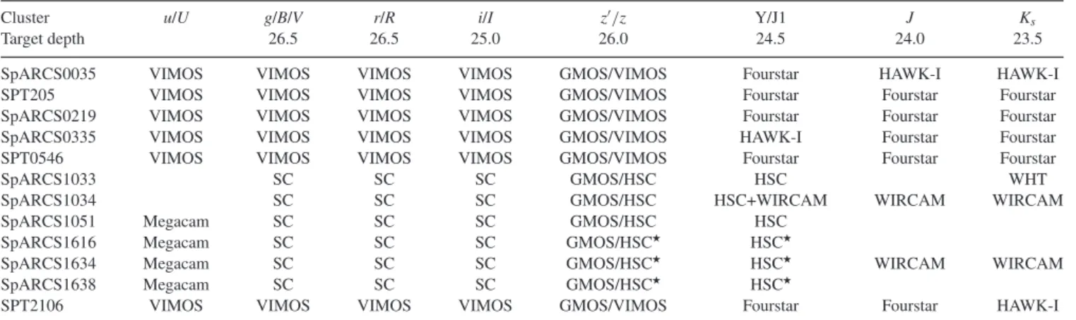
Figure 8. The top image shows the red end of a sky-subtracted, two-dimensional spectrum from a single slit in mask GS205ALP001-02. Strong residuals are evident atλ >9500 Å as positive flux near the bottom of the frame, and negative flux near the top. This is due to charge diffusion from the n&s pair, as described in the text. To correct this, we create a template from a stack of sky-subtracted spectra, with continuum removed. This is shown in the middle panel, where the charge diffusion residuals are the only feature. After applying this correction to the data, we obtain the spectrum in the bottom panel. The grey scale is the same in all three images, ranging from−10 to+10 counts.

only the residuals due to charge diffusion, as shown in the middle spectrum of Fig.8.

What remains is to subtract this ‘master residual’ from the data, after appropriate rescaling. The amplitude of the residual is expected to be directly proportional to the flux in the corresponding sky spectrum, since this light dominates over the object and uniformly fills the slit. Thus, we measure the mean signal of each column in the sky spectrum that corresponds to a given science slit. Pixels with DQ flags, or sky values<0 or>5000, are masked. The average is taken only of the four central rows, which are relatively free from science target flux. We take the ratio of this average to the average of the same pixels in the combined sky spectrum, and use this to scale the master residual image. Finally, this scaled image is subtracted from the science data, atλ >8000 Å, where the effect is significant. The resulting science spectrum is free from these residuals, as shown in the bottom panel of Fig.8. The subtracted flux is stored in a new extension labelled ‘REDFIX’.

Three masks taken in early 2015 (two in COSMOS-221 and one for COSMOS-125) had to be dealt with separately. The charge diffusion here is larger than predicted by the simple scaling of the master residual described above.5_{Having identified this, these}

images were excluded from the master residual described above. To deal with these frames, a similar process was followed, but using stacked residual frames in bins of date,xccdandyccd. With significant

trial and error to choose appropriate bin sizes, corrections were found that work reasonably well for these three masks.

The effect is also present on the EEV images from GMOS-N. It does not present as much of a problem here, as the detector sensi-tivity has died off by the time the effect becomes most problematic, beyond∼9600 Å. Since we do not plan to obtain any band-shuffle masks with the EEV detectors on GMOS-N, a different procedure is required to remove the continuum from the residual stack. We take the band-shuffle continuum image described above and first rescale in the spatial direction to match the EEV pixel size, using a second-order spline. We then scale the intensity as a function of wavelength by the ratio of the EEV sensitivity relative to the Hama-matsu, using standard star observations. This serves to adequately model the average EEV continuum image, at least forλ >8000 Å. This is subtracted from the combined microshuffle data as for the Hamamatsu observations, to produce an appropriate master residual frame.

5_{This may be related to a detector controller problem that was noted by} Gemini a few weeks later, and which led to a much more severe charge smearing effect.

3.4 Extraction and flux calibration

We fully reduce each mask, including wavelength calibration, sky subtraction, and (where necessary) charge diffusion correction, and then median combine the slits usinggemcombine, first rejecting the lowest and highest pixels. The reduced, two-dimensional image of each slit is 3high, with an object spectrum at the top and an inverted spectrum at the bottom. We first compute an average spatial profile of the slit, by computing the median within 8000< λ <9750 Å, rejecting bad pixels using the DQ mask. We ignore the two pixels closest to either edge of the slit. This profile is fit with two Gaussian distributions, one with amplitudeAand the other with amplitude

−A. Both are forced to have the same width,σ, and to be separated by a fixed amount given by the nod distance of 1.45. Next, we repeat the process for small intervals of wavelength (typically 250 or 500 Å), but keepingσfixed. Thus, we fit for only two parameters at each wavelength bin: the overall normalization, A(λ), and the position of the bottom peak,y(λ). Finally, we ploty(λ) as a function of λ, and fit a polynomial to it with 2σ rejection. The order of the polynomial, and the wavelength range of the fit, is determined interactively by the user. Typically, the order is 0–2, and the fit is done over 6500< λ <9500 Å.

The spectral extraction is then a weighted sum of all pixels in a column (again omitting the top and bottom two pixels), where the weights are given by the double Gaussian function with vertical position at each wavelength given by the polynomial fit. Thus, most of the weight is given to the pixels at the centre of each spectrum. The amplitude is irrelevant, but the sign of the function ensures that the spectrum with negative flux is subtracted from the one with positive flux.

The extraction is made via a tool which shows the median ex-traction profile, the plot ofy(λ) versusλas well as the fit, the fit locations of both Gaussian peaks overlaid on the two-dimensional spectrum, and the spectrum extracted from this fit. Polynomial or-der, wavelength coverage, and binning are chosen interactively to ensure a good fit to each spectrum. The extraction parameters are stored in the header of the extracted spectrum.

Spectral flux standard observations are taken once each semester. The standards are reduced using the same pipeline described above, including the QE correction for GMOS-S. As these are not observed in n&s mode, however, sky subtraction is done classically by defin-ing a sky region adjacent to the source. The extracted spectrum is compared with tabulated values in theIRAFdata base to generate a

sensitivity function which is then applied to the extracted science data.

Bands of telluric absorption at 6850< λ/Å∼6940 (Bband), 7550 < λ/Å < 7710 (A band), 8120 < λ/Å < 8370, and

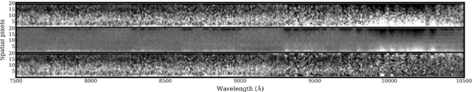
Figure 9. Sample data are shown for five galaxies in a range ofzmagnitudes, indicated by the numbers on the right. Redshifts are given in the top left corner of each panel, and key identifiable spectral features are labelled (Calcium H and K, HδandG-band absorption, and [OII] emission). The stamps on the right show thez-band image, scaled to the minimum and maximum counts within the subimage. The red and yellow rectangles show the predicted slit position in both nod positions. To the left are the one-dimensional (top) and two-dimensional (bottom) reduced spectra, after all reduction including sky subtraction, charge diffusion correction, and telluric/sensitivity correction (the latter applied only to the one-dimensional spectrum). All spectra shown here are from 7.2 ks of exposure, and the one-dimensional spectra are convolved with a 5 pixel (∼20 Å) boxcar filter. For the faintest two galaxies, the goal is to build up the S/N by re-observing in multiple masks, with up to 54 ks exposure by the end of the survey.

8940< λ/Å<9840 are corrected using anIRAFpackage that

cross-correlates telluric features from our standard stars to compute a shift and scalefactor before subtracting from the data. This does not pro-vide a perfect correction for the red features (λ >8000 Å), as these lines vary on short time-scales. Starting in 2016B, we have been including one bright star in each mask. By fitting templates to those stars we expect to derive a telluric correction which is applicable to all spectra in that mask. For earlier observations, we are exploring ways to use the existing data to derive improved corrections.

3.5 Final spectra and science analysis

In Fig.9, we show some sample images and extracted one- and two-dimensional spectra for five targets after just 7.2 ks exposure. A range of magnitudes are shown; the faintest galaxies (z>23.5) will ultimately accrue up to 54 ks of exposure by observing in multiple masks. The two-dimensional spectra shown are sky sub-tracted and corrected for charge diffusion. In these images, there is a positive- and negative-flux copies of the spectrum due to the n&s technique. Note the spectrum is free from sky line residuals. The one-dimensional spectra are extracted as described in Section 3.4, including sensitivity calibration and preliminary telluric correction. Four of the spectra shown here show a strong [OII] emission line,

clearly identifiable in both the one- and two-dimensional spectrum.

The top spectrum is a pure absorption line system, with the Ca H+K lines easily identifiable atλ∼8200 Å.

Preliminary redshifts are being determined independently us-ing theRUNZcode,6and an updated version of the DEEP2spec1d

pipeline (Newman et al.2013). Future improvements will include adding rest-UV templates generated from our own data.

Stellar masses for the sample will be derived from SED fitting to multiwavelength photometry, including deep [3.6]µm imaging. For those clusters which currently lack sufficiently deep data, we have shown (Muzzin et al.2012) that corrections forM/Lbased on D4000 are sufficient to obtain masses to within a factor∼2 of those derived from SED fitting. This requires D4000 to be measured to within 20 per cent precision (corresponding to S/N∼0.7 pixel−1_),

which will be achievable for every galaxy for which we can get a redshift.

To measure the quiescent fraction, we need to classify our galax-ies. This is best done using colour–colour diagrams spanning the rest-frame near-ultraviolet to NIR, which does an excellent job of separating dusty star-forming galaxies from truly passive galaxies (e.g. Muzzin et al.2013a; Mok et al.2013; Arnouts et al.2013).