Gerhard H. Jirka1, Tobias Bleninger1, Richard Burrows2, Torben Larsen3
Environmental Quality Standards in the EC-Water Framework
Directive: Consequences for Water Pollution Control for Point
Sources
Abstract
The „combined approach“ in the new EC-Water Framework Directive (WFD) consisting of environmental quality standards in addition to emission limit values promises improvements in the quality characteristics of surface waters. However, the specification of where in the wa-ter body the environmental quality standards apply is missing in the WFD. This omission will limit its administrative implementation. A clear mixing zone regulation is needed so that the quality objectives of the WFD are not jeopardized. This need is demonstrated using the ex-amples of point source discharges into rivers and coastal waters, respectively. Furthermore, water authorities will have to make increased use of predictive modeling techniques for the implementation of the “combined approach”.
Key words: water pollution control, surface waters, pollutants, water framework directive, effluents, mixing zone, water quality models
1. Introduction
The new EC-Water Framework Directive (WFD, 2000) has the objective of an integrated catchment-oriented water quality protection for all European waters with the purpose of at-taining a good quality status by the year 2015. The water quality evaluation for surface waters shall rely predominantly on biological parameters (such as flora and fauna) - however, aided by hydromorphological (such as flow and substrate conditions) and physico-chemical quality components (such as temperature, oxygen or nutrient conditions) - and on specific pollutants (such as metals or synthetic organic compounds). A good chemical quality status is provided when the environmental quality standards are met for all pollutants or pollutant groups. The WFD defines new strategies against water pollution as a consequence of releases from point or diffuse sources. A new aspect of the EC water policy is the “combined approach”, i.e. both limitations on pollutant releases at the source due to promulgation of emission limit
val-1.
European Water Management Online
Official Publication of the European Water Association (EWA) © EWA 2004
Ragas et al. (1997) have reviewed the advantages and disadvantages of different control mechanisms in the permitting processes of releases into surface water. Emission limit values (ELV) present a direct and effective method for the limitation of pollutant loadings by re-stricting the concentration for the mass flux of specific pollutants. ELVs are preferred from an administrative perspective because they are easy to prescribe and to monitor (end-of-pipe sampling). From an ecological perspective, however, a quality control that is based on ELVs alone appears illogical and limited, since it does not consider directly the quality response of the water body itself and therefore does not hold the individual discharger responsible for the water body. To illustrate that point consider a large point source on a small water body or several sources that may all individually meet the ELVs but would accumulatively cause an excessive pollutant loading. Environmental quality standards (EQS), set as concentration values for pollutions or pollutant groups, that may not be exceeded in the water body itself (WFD, 2000) have the advantage that they consider directly the physical, chemical and bio-logical response characteristics due to the discharge and therefore they put a direct responsi-bility on the discharger. But a water quality practice that would be based solely on EQSs could lead to a situation in which a discharger would fully utilize the assimilative capacity of water body up to the concentration values provided by the EQSs. Furthermore, the water quality authorities would be faced with additional burdens because of a more difficult moni-toring – where in the water body and how often should be measured? – in the case of existing discharges or due to the increased need for a prediction modeling in case of new discharges. The “combined approach” in the WFD combines the advantages of both of these quality water control mechanisms while largely avoiding their disadvantages.
The objective of this contribution is a critical analysis regarding the practical implementation of the “combined approach” for water quality management due to point sources in surface wa-ters. In particular two questions of central importance to the practice of water authorities will be explored for the examples of discharges into rivers and coastal waters, respectively:
1) Where in the water body relative to the discharge point do the EQS-values apply? Since the WFD provides no specific guidance on that question two extreme interpretations might be applied. First, the EQS-values apply immediately after the discharge with the idea that the whole water body would then be in a state of a good chemical status at every location at every time as indicated by the EQS-values. In that case, however, the EQS-values would be syn-onymous with the ELV-values! Secondly, the EQS-values apply after complete mixing (for river discharges) or at some sensitive area, e.g. the adjacent beach (for coastal discharges). Since the actual physical mixing processes in rivers and in most other water bodies take place gradually leading to a “discharge plume”, as will be shown in the following, considerable ar-eas in the water body would be affected by concentrations above the EQS-values and would have to be considered as “sacrificial regions”, in which a good chemical status would no longer be provided. Considering these two extreme interpretations it is obvious that a com-promise, in form of a clear mixing zone regulation, is necessary.
2) Which procedures shall be used during the permitting process to demonstrate that the dis-charge will in fact meet the relevant EQS-values in addition to the ELVs? Not only for exist-ing, but especially also for future, discharges does it seem necessary that predictive models
that describe the physical mixing and transport as well as chemical and biological transforma-tion processes be applied so that the water authorities can in fact administer the “combined approach”. In addition it is necessary to consider different hydrological situations (which current or flowrate is relevant?) or physical conditions (which season is relevant, e.g. for den-sity stratification?).
2. Mixing processes for point sources in rivers and coastal waters
When performing design work and predictive studies on effluent discharge problems, it is im-portant to clearly distinguish between the physical aspects of hydrodynamic mixing processes that determine the fate and distribution of the effluent from the discharge location, and the administrative formulation of mixing zone regulations that intend to prevent any harmful im-pact of the effluent on the aquatic environment and associated uses.
The hydrodynamics of an effluent continuously discharging into a receiving water body can be conceptualized as a mixing process occurring in two separate regions. In the first region, the initial jet characteristics of momentum flux, buoyancy flux (due to density differences), and outfall geometry influence the effluent trajectory and degree of mixing. This region, the "near-field", encompasses the buoyant jet flow and any surface, bottom or terminal layer in-teraction. In this near-field region, outfall designers can usually affect the initial mixing char-acteristics through appropriate manipulation of design variables. As the turbulent plume trav-els further away from the source, the source characteristics become less important and the far-field is attained. In this region ambient environmental conditions will control trajectory and dilution of the turbulent plume through buoyant spreading motions, passive diffusion due to ambient turbulence, and advection by the ambient, often time-varying, velocity field.
2.1 Mixing processes for point sources in rivers
For river discharges the problem can be reduced in first order to so-called “passive” sources for which the input momentum and buoyancy effects are of lesser importance and mixing is controlled by the advective and diffusive properties of the ambient flow regime with a result-ing discharge plume that follows the prevailresult-ing current. Thus, the problem is considered as a “far-field” effect with passive source characteristics. Research during the last 40 years has led to a solid understanding of the mixing dynamics in rivers as summarized in several text-books or manuals (e.g., Fischer et al., 1979; Holley and Jirka, 1986; Rutherford, 1994).
1.
European Water Management Online
Official Publication of the European Water Association (EWA) © EWA 2004
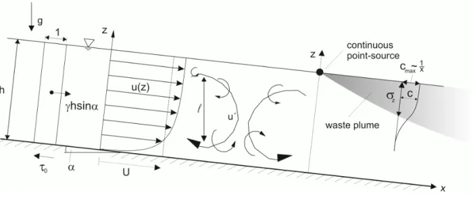
The friction velocity u = o/ , is obtained on dimensional grounds, so that u = ghS. u is therefore the major quantity characterizing the fluctuating eddy velocities u' in channel flows, u' ~ u , as has been confirmed by many measurements (Nezu and Nakagawa, 1993). It is related to the average velocity U by the frictional properties (roughness) of the bottom and is typically about 5 to 10% of U, u = (0.05 to 0.10)U, with higher values for rough beds.
Fig. 1: Longitudinal section along an inclined river flow with turbulent flow structure and assumed continuous point sources at the water surface
The large eddies that correspond to the depth of the base flow, +~ h, are most effective for the mixing. Moreover, the eddy structure is characterized by a certain spatial anisotropy, their extent in the vertical direction z is more strongly limited than that in the horizontal direction y that lies transversely to the flow direction x. In summary, the following expressions for the turbulence diffusivities result from the above: The vertical eddy diffusivity Ezis
z z
E = u h (1)
where z= 0.07 ±50% (Rutherford, 1994) and the horizontal diffusivity Ey
y y
E = u h (2)
where y= 0.5 ±50% (Fischer et al., 1979) for rivers with moderate variability, thus without
strong meanders and without lateral dead water zones.
If a continuous point source is considered at the water surface a mass plume will evolve as is shown in vertical section in Fig. 1 and in plan view in Fig. 2. The pollutant plume spreads both vertically and transverse. Characteristic for such diffusion processes is the approximately
water surface and at the river bank. The standard deviation describes here a local value c = e-1/2 cmax = 0,61 cmax and is a practical indicator for plume width.
The distance Lmv to the location of complete vertical mixing of the plume is often defined as
being to the point when the concentration at the bed becomes 90% of the surface concentra-tion and this can be determined by the method of images (Fischer et al., 1979)
2 mv z Uh L 0.4 E = (3)
Using Eq. 1 ( = 0.07) and strong roughness, u =0.10U, the distance to the location of complete vertical mixing is given by
mv
L 50h (4)
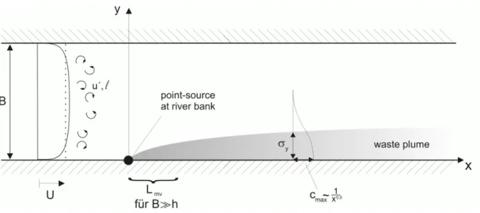
The transverse spreading of a continuous point source in a wide river flow (B >> h) is out-lined in fig. 2. The longitudinal coordinate follows in this case any river curvature and a con-stant rectangular cross-section is assumed. The distance Lmh to the location where complete
horizontal mixing over the river cross-section takes place is 2 m h y UB L 0.4 E = (5)
With y= 0.5 and for strong roughness one obtains
mh
B
L 8 B
h (6)
It should be noted that these simple equations for the estimation of complete mixing, Eq. 4 and 6, respectively, are a) independent of the river velocity and b) primarily governed by the
river morphology. The first is because the turbulent mixing coefficients Ey and Ez scale
di-rectly with the mean velocity U! Comparison of the two formulas shows that in a wide river (B >> h), the length for complete vertical mixing is always rather small as has been indicated in Fig. 2. Furthermore, in the initially three-dimensional mixing process (until the location where complete vertical mixing takes place) the drop-off of the maximum mass concentration
is relatively fast, cmax ~ x-1 (Fig. 1), while it occurs more gradually in the vertically mixed,
1.
European Water Management Online
Official Publication of the European Water Association (EWA) © EWA 2004
Fig. 2: Transversal spreading for a continuous point-source located at the bank of a wide river flow (B>>h), plan view
Two examples are used for the practical illustration of the mixing dynamics of point sources in rivers: i) Large river (approximately River Rhine near Karlsruhe, Germany, at average dis-charge), B = 250 m, h = 3 m, and ii) small river, B = 5 m, h = 0.5 m. The calculations given in Table 1 show that complete vertical mixing occurs reasonably fast (150 m and 25 m, re-spectively), while complete lateral mixing requires considerably larger distances (160 km and 0.4 km, respectively)!
Table 1: Examples for the complete mixing of a passive point source located at water surface and at bank of a river
Example B/h Distance to complete mixing
Vertical Lmv Horizontal Lmh
i) Large River
B = 250m, h = 3m 80 150 m 160 000 m ii) Small River
B = 5m, h = 0,5m 10 25 m 400 m
Several comments are in order: 1) The distance to complete vertical mixing will be somewhat reduced if the finite dimensions of the discharge opening are considered or if the source loca-tion is varied within the water column, e.g. located at mid-depth. Thus, the discharge design can play a certain role in this initial region. 2) The design features play a lesser role regarding
the passive lateral spreading in the far-field. Only the lateral position of the discharge point is a potential factor: e.g. if the source is located in the center of the river the distances for com-plete mixing are reduced by a factor 4 (since B/2 is used instead of B in Eq. 5 as the control-ling lateral dimension). Beyond that, only the flow conditions in the river are decisive: For uniform flow conditions the estimation according to Eq. 6 would be somewhat low, while for strongly heterogeneous conditions – e.g. strong river meanders, or lateral constrictions that induce secondary flows – the actual distance might be somewhat shorter. 3) Both vertical and lateral complete mixing can be influenced by active mixing processes in the near-field of the discharge. Active mixing by momentum jets – especially in case of multiple diffuser dis-charges in rivers (e.g. Schmid and Jirka, 1999) – and buoyancy effects due to density differ-ences lead, in general, to a reduction of the length for complete mixing. Models for the classi-fication and prediction of these mixing complexities are available (e.g. Jirka et al., 1996). Regardless of potential amplifications and complexities, the following rules of thumb apply for the mixing properties of point sources in rivers: 1) Complete vertical mixing is a rapid process with maximal dimensions of a few decades of the water depth. 2) Complete lateral mixing requires large distances. For typical river morphology (B/h = 10 to 100) the complete mixing will require from 100 to 1000 river widths (see also Endrizzi et al., 2002).
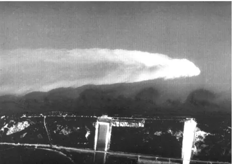
These analytical predictions for the delayed lateral mixing that are based on the description of the turbulent river flow properties have been confirmed through numerous field observations, in particular aerial photographs of “visible” plumes, taken from a period before recent source reductions were imposed, as shown in Fig. 3.
2.2 Mixing processes for point sources in coastal waters
Point sources in coastal waters in the form of offshore submerged sea outfalls can be used for many purposes and in different settings. Their most prevalent use is for discharges of sewage flows from municipal waste treatment plants (with various degrees of treatment), but they can also be used for industrial or mining effluents, for cooling water discharges from thermal-electric power plants, or for brine effluents from desalination installations. The coastal envi-ronment can be highly diverse, ranging from a coast with unidirectional currents, to coastal bays with circulating flows, to estuaries with tidal variability and/or riverine influences.
1.
European Water Management Online
Official Publication of the European Water Association (EWA) © EWA 2004
Fig. 3: Aerial photograph (ca. 1960) of an industrial discharge located near the middle of the regulated River Rhine upstream of Lake Constance (Bodensee). The gradual lateral plume growth of the pollutant is typical for mixing processes in rivers. (Photograph courtesy of D. Vischer, Zurich)
The mixing behaviour of a submerged sea outfall is governed by the interplay of ambient conditions (bathymetry, flow and density structure, as for the river application, but com-pounded by the further environmental disturbances of oscillatory tidal and wind driven cur-rent streams) in the receiving water body and by the discharge characteristics. A review of these processes has been given by Fischer et al. (1979), Wood et al. (1993), or Jirka and Lee (1994). The discharge conditions relate to the geometric and flux characteristics of the sub-merged outfall installation. (Discharges directly at the shoreline, e.g. through a canal, will not be considered here.) For a single port discharge the port diameter, its elevation above the bot-tom and its orientation provide the geometry; for multiport diffuser installations the arrange-ment of the individual ports along the diffuser line, the orientation of the diffuser line, and construction details represent additional geometric features. The flux characteristicsare given by the effluent discharge flow rate, by its momentum flux and by its buoyancy flux. The buoyancy flux represents the effect of the relative density difference between the effluent dis-charge and ambient conditions in combination with the gravitational acceleration. It is a
measure of the tendency for the effluent flow to rise (i.e. positive buoyancy) or to fall (i.e. negative buoyancy).
The “near-field” of a sea outfall is governed by the initial jet characteristics of momentum flux, buoyancy flux, and outfall geometry as these influence the effluent trajectory and mix-ing. Flow features such as the buoyant jet motion and any surface, bottom or terminal layer interaction also take place. In the near-field region, outfall designers can usually affect the initial mixing characteristics through appropriate manipulation of design variables. For exam-ple, Fig. 4 shows a laboratory demonstration of a discharge jet/plume motion that is trapped by the ambient density profile below the water surface leading to a plume spreading at a ter-minal level. This is a frequently employed design strategy for sewage discharge during sum-mer stratification in coastal waters. Recent field data (Carvalho et al., 2002) provide further evidence of such plume phenomena. As the turbulent plume travels further away into the “far-field”, the source characteristics become less important. Conditions existing in the ambient environment will control trajectory and dilution of the turbulent plume through buoyant spreading motions, passive diffusion due to ambient turbulence, and advection by the ambi-ent, usually time-varying velocity field. Fig. 5 gives an infrared image of the continuous plume produced at the water surface by a submerged cooling water discharge.
In total, the discharge plume and associated concentration distributions generated by a con-tinuous efflux from a sea outfall can display considerable spatial detail and heterogeneities as well as strong temporal variability, especially in the far-field. This has great bearings on the application of any water quality control mechanisms.
1.
European Water Management Online
Official Publication of the European Water Association (EWA) © EWA 2004
Fig. 5: Surface plume in a long shore coastal current produced by a submerged sea outfall. The infrared image shows the plume produced by the cooling water discharge from a power plant at the western coast of Florida.
In the general case, with notable (oscillatory) tidal current motions and variable wind field creating differing shear currents, the delineation of the 'mixing zone' can become much more difficult to define and may call for adoption of suitable 'statistical' descriptors (i.e. drift asso-ciated with spring-tide currents and 1-in-10 year onshore wind, etc). In these cases the mixing zone may be large but large sub-zones within this region may only experience sporadic (and transient) exposure to the dispersing plume.
A critical issue in respect of the management of coastal water bodies is likely to be the (de-gree of) segregation of the mixing zone from such prime use areas (within the water body) as shellfisheries or bathing waters etc. Such problems are likely to be more acute in respect of the impacts of intermittent shoreline (storm overflow) discharge fields not addressed specifi-cally herein.
3. Consequences for implementation of the “combined approach”
3.1 Mixing zone regulations
The mixing processes due to discharges into water bodies occur according to well understood physical principles, as has been shown above, and lead to a spatial and temporal configuration of the mass plume and the associated concentration distribution. To what degree do the water quality control measures of the new EC-WFD, in particular its “combined approach” consist-ing of emission limit values (ELV) and environmental quality standards (EQS), correspond to these physical facts?
The relevant values for ELV and EQS for various pollutants and pollutant groups can be found in different directives of the EC (see e.g. Appendix IX of the WFD) or of the national
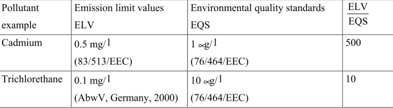
authorities. By way of example for further analysis, Table 2 contains the values for two chemical pollutants (cadmium and triochlorethane). The ratio ELV/EQS is 10 for triochlore-thane and 500 for cadmium. The range of 5 to 1000 is typical for most chemical as well as physical parameters, such as heat (temperature). This ratio describes the impact of the pollut-ants on the ecosystem, since the ELV is considered to protect against acute (lethal) effects on organisms, while the EQS is supposed to prevent long-time chronic influences. The ratio also expresses the necessary dilution that must be attained through physical mixing or - to some extent - through biological decay and chemical transformation processes.
Table 2: Examples for emission limit values (ELV) and environmental quality standards (EQS) for two selected pollutants
Pollutant example
Emission limit values ELV
Environmental quality standards EQS ELV EQS Cadmium 0.5 mg/l (83/513/EEC) 1µg/ l (76/464/EEC) 500 Trichlorethane 0.1 mg/ l (AbwV, Germany, 2000) 10 µg/ l (76/464/EEC) 10
There can be other ways of prescribing ELV-values, namely through the specification of a “best available technology (BAT)”. For example, for sea outfalls of sewage this may be de-scribed as some form of treatment, at least primary, or enhanced (e.g. chemically) primary, or a secondary biological treatment stage for nitrogen removal, or a tertiary stage for phosphorus removal. The requirement may be set by national authorities depending on type of coastal water body and its use (fisheries or recreation) or on sensitive ecological zones. In general, such BAT requirements assure a certain degree of nutrient removal. Other indicator parame-ters, such as bacteria or viruses, are also reduced in the treatment process. For example, while
the typical total coliform count for raw sewage ranges from 106 to 108/100ml it gets reduced
by a factor 100 to 1000 during secondary and by 1000 to 10,000 during tertiary treatment (Larsen, 2000). Assuming an average factor of 1000 the effluent values for total coliform
1.
European Water Management Online
Official Publication of the European Water Association (EWA) © EWA 2004
Both measures, concentration values and removal degrees are useful to reduce and control water pollution, but where do these values apply? The „end-of- pipe“ specification for the ELV is clear and unequivocal in Art. 2 (40) of the WFD:
„The emission limit values for substances shall normally apply at the point where the emissions leave the installation, dilution being disregarded when determining them“.
Surprisingly, and quite illogical from the viewpoint of the physical features of the mixing processes, the WFD does not provide any information on the spatial application of the EQS-values. It also does not oblige the national authorities to establish such specification. There-fore, it must be expected that considerable uncertainties and highly variable interpretations or monitoring methods will occur in the practice of water authorities, both as regards the con-tinuing approval of existing discharges as well as the permitting of new ones. The “combined approach” that appears sensible for an integrated ecological water pollution control is in dan-ger of being by-passed or undermined in its practical implementation.
From discussions with personnel from regional water authorities the authors know of two ex-treme interpretations regarding this omission in the WFD:
1) The EQS-value shall be applied “as near as possible” to the discharge point in order to obtain a good chemical status in an area as large as possible. This highly restrictive interpretation negates the fact that the physical mixing process cannot be reduced to ex-tremely small areas (in the limit this approaches an “end-of-pipe” demand for EQS!), but re-quires a certain space – in particular for imposed high ELV/EQS ratios. It undermines the balanced objectives of the “combined approach”.
2) In case of rivers, the EQS-value applies after “complete mixing in the water body”. However, as was shown in the preceding section the longitudinal extent of the pollut-ant plume until full lateral mixing is attained can be considerable, even in small rivers. This highly generous interpretation could therefore lead to a condition that large regions within a pollutant plume of the point source would be exposed to concentration values above the EQS and would, therefore, represent “sacrificial stretches”. A similar evaluation can be found in a recent German strategy report on water research (DFG-KOWA, 2003): “The occasional as-sumption that environmental quality standards apply only after complete mixing leads in most water body types to intolerably large distances since mixing processes usually occur gradu-ally…”.
3) In the case of coastal discharges, the EQS-value is supposed to apply “after the completion of initial mixing” or “at the beach” or “at the water surface”. All such qualitative statements have specific deficiencies, that make them either unenforceable or overly generous and likely to create sacrificial areas with high concentration levels not meeting a good quality status.
Thus, the new “combined approach” concept of the WFD is lacking a clear and factually cor-rect mixing zone regulation that preserves the water quality objectives of the “combined ap-proach” and accounts for the physical aspects of the mixing processes. Therefore, a future amendment of the EC-WFD and national regulations for its implementation, respectively,
should contain the following approximate wording:
„The environmental quality standards apply in the case of point sources outside and at the edge of the mixing zone. The mixing zone is a spatially restricted region around the point source whose dimensions shall be specified either according to water body type and use or on an ad-hoc basis.”
The mixing zone defined in the above statement is a regulatory formulation with the follow-ing general attributes: 1) The term “mixfollow-ing zone” signifies explicitly that mixfollow-ing processes require a certain space. 2) The term “spatially restricted” should guarantee that the mixing zone shall be minimized by the regulatory authority for the purpose of attaining the environ-mental quality goals. 3) While the mixing zone includes a portion - namely the initial one - of the actual physical mixing processes, these processes will continue beyond the mixing zone where they lead to further concentration drop-offs in the pollutant plume below the EQS-values. 4) The definition is restricted to “point sources” since diffuse sources usually do not contain clearly distinct mixing processes.
The regulatory concept of mixing zones can also be found in the water quality regulations of other countries. As an example, the U.S. Environmental protection Agency defines in its Wa-ter Quality Handbook “… the concept of a mixing zone as a limited area or volume of water where initial dilution of a discharge takes place” (USEPA, 1994). A number of supplemen-tary restrictions further define this water quality control principle such as “… the area or vol-ume of an individual mixing zone … be limited to an area or volvol-ume as small as practicable that will not interfere with the designated uses or with the established community of aquatic life in the segment for which the uses are designated," and the mixing zone shape be "… a simple configuration that is easy to locate in the body of water and avoids impingement on biologically important areas."
Once the principle of a mixing zone has been adopted and defined in the EC-WFD and/or na-tional regulations it is also necessary that nana-tional water authorities provide clear guidance for the actual specification of mixing zone dimensions. Two major possibilities exist here: a) Specification of numeric mixing zone dimensions according to water body type and biological characteristics:
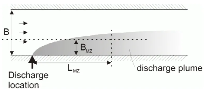
In the case of discharges into a river (see Fig. 6), the width of the mixing zone BMZ can be
1.
European Water Management Online
Official Publication of the European Water Association (EWA) © EWA 2004
Fig. 6: Example of regulatory mixing zone specifications for discharges into rivers: Width of mixing zone BMZ, and/or length of mixing zone LMZ, both defined relative to the river width B.
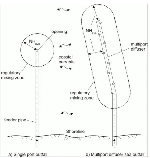
In the case of coastal discharges with submerged offshore sea outfalls it seems advisable to constrain the mixing zone to a limited region around the outfall in which the initial buoyant jet mixing is dominant (see Section 2.2). In that fashion the EQS-values can be achieved within short distances. Thus the following specification appears effective: “The mixing zone is a volume with vertical boundaries in the coastal water body that is limited in its horizontal extent to a distance equal to N multiples of the average water depth Have at the outfall
loca-tion and measured in any direcloca-tion from the outfall structure.” Thus, for a single port outfall this would be a cylindrical volume with the port in its center (Fig. 7a). For a multiport dif-fuser outfall with many ports arranged along a straight difdif-fuser line it would be a rectangular prismatic volume with attached semicircular cylinders at the diffuser ends located along the diffuser line (Fig. 7b). For diffusers with a curved diffuser line or piecewise linear sections the volume would follow the diffuser line. The value N would typically be in the range of at least 1 to about 10 and set by the regulatory authority according to local water use and eco-logical sensitivity. For highly sensitive waters the minimum of 1 should be set. Common values for most coastal waters might be N = 2 to 3.
b) Specification of mixing zone dimensions in an ad-hoc manner:
After prior ecological evaluations or predictions the discharger can request the authority for a mixing zone with a certain dimension with the claim that this would guarantee an integrated water quality protection. Based on its own examinations the authority can agree with that proposal or else demand further restrictions.
Fig. 7: Example of regulatory mixing zone specification for offshore submerged coastal discharges: The horizontal extent of the mixing zone is defined by some multiple N of the average water depth Have at the sea outfall.
3.2 Increased use of modeling techniques for mixing processes
In order to demonstrate compliance with the EQS-values it appears that both dischargers as well as water authorities must increase the application of quantitative predictions of substance
1.
European Water Management Online
Official Publication of the European Water Association (EWA) © EWA 2004
There are several diagnostic and predictive methodologies for examining the mixing from point sources and showing compliance with EQS-values:
1) Field measurementsor tracer tests can be used for existing discharges in order to verify whether EQS-values are indeed met. Field measurements are costly, often difficult to per-form, and usually limited to certain ambient conditions. Frequently, they must be supported through mathematical model predictions, on one hand, to establish a clear linkage to the con-sidered discharge (especially if more than one discharge exists), and on the other hand, to synthesize conditions allowing for variabilities in the hydrological or oceanographic condi-tions or in the effluent rates.
2) Hydraulic model studies replicate the mixing process at small scale in the laboratory. They are supported by similarity laws and are quite reliable if certain conditions on minimum scales are met as has been demonstrated in the past. But just like field tests, they are also costly to perform and inefficient for examining a range of possible ambient/discharge interac-tion condiinterac-tions.
3) Simple analytical equations or nomograms (e.g. Rutherford, 1994; Holley and Jirka, 1986) are often satisfactory to predict reliably the mixing behavior of a pollutant plume. For example, the maximum pollutant concentration cmax as a function of distance x along the flow
for a passive point source at the bank of a river (see Fig. 2) is given by
co max y Q c 2 h 4 E Ux = (13)
where Qco is the pollutant mass flux of the source (mass/time) and Eyis the lateral turbulent
diffusivity from Eq. 2. The factor 2 on the right hand side signifies the reflection effect of the impermeable river bank. In many river applications with relatively uniform cross-sections Eq. 13 would be satisfactory for a conservative prediction, possibly combined with parameter
sensititivity studies (see coefficient y in Eq. 2) in order to predict the maximum pollutant
concentration along the bank and to demonstrate compliance with the EQS-values. Simple amplifications of Eq. 13 in the form of a stream tube method (see Fischer et al., 1979) are available for strongly meandering and non-uniform river sections. Equally simple equations or analytical expressions can be applied for the initial buoyant jet/plume mixing plans of sin-gle or multiport submerged discharges (e.g. Jirka and Lee, 1994). They have been validated through numerous data comparisons from laboratory or field measurements as shown in the existing literature.
4) Mixing zone models are simple versions of more general water quality models. They de-scribe with good resolution the details of physical mixing processes (mass advection and dif-fusion), but are limited to relatively simple pollutant kinetics by assuming either conservative substances or linear decay kinetics. This is acceptable for most applications, since residence times in the spatial limited mixing zones (see previously mentioned specifications) are typi-cally short so that chemical or biological mass transformations are usually unimportant. As for all computer-based models that are concerned with environmental problems – here with
water quality as a common good! – the scientific transparency of the predictive models is es-sential. That means not only that the governing equations and all relevant assumptions must be clearly published but also the actual calculation module must be available as public do-main software and thus scientifically verifiable. User interfaces as well as pre- and post-processing modules can, of course, be added, developed and distributed in a for-profit manner in an open market.
Undoubtedly, the main problem in the application of mixing zone models is the estimation of its applicability by the user. In particular, simple model types are often limited to certain flow situations. Model assumptions and limitations must be clearly stated by the model de-veloper. But even then it may be difficult for the user with limited experience in these com-plex processes of fluid mechanics to judge whether a model is applicable for a specific situa-tion. The application of expert systems seems advisable for that problem. An expert system can lead the user in sequential steps through data acquisition, it performs the selection of a specific sub-model or predictive equation depending on the physical situation, it provides the graphical display and interpretation of the predictive values with regard to the compliance with EQS-values and mixing zone regulations, and finally it may provide recommendations regarding additional sensitivity studies or design changes for the optimization of the mixing process.
Ragas (2000) provides a comparison of different mixing zone models. The mixing zone model CORMIX (Doneker and Jirka, 1991; Jirka et al, 1996), in particular, is characterized by its wide applicability to many water body types (rivers, lakes, estuaries, coastal waters) and has been successfully used for water quality management under different regulatory frameworks.
5) General water quality models may be required in more complex situations. In simple water bodies, such rivers, coastal regions or estuaries with well defined uni-directional current regimes or with simple reversals, and with moderate pollutant loadings, the use of mixing zone models alone may suffice to arrive at, or to evaluate, a design of a point source discharge that meets regulations. However, in coastal regions with multiple current regimes (inertial, tidal, wind- or buoyancy driven) and in rivers and coastal regions with large pollutant load-ings, especially where several sources may interact and additional diffuse sources may exist, mixing zone models must be supplemented by larger-scale (far-field) transport and water quality models. The latter are capable of prediction over greater distances in the water body the concentration distributions for different pollutants, but also for nutrients and other
bio-1.
European Water Management Online
Official Publication of the European Water Association (EWA) © EWA 2004
QUAL-2 of the U.S. EPA, and the model RWQM1 of the International Water Association are all examples of general water quality models. Such models also form the basis of manage-ment procedures for attaining a good quality status in the case of multiple sources, i.e. by. fol-lowing the principle of a distributed waste load allocation for individual water users
4. Conclusions
The “combined approach” in the new EC-WFD appears to be logical in its intention toward a consistent improvement of water quality. However, the wording in the WFD for the actual implementation of the “combined approach” is vague and incomplete. For this reason, the further implementation into national law and administrative procedures is in jeopardy and the new approach will be avoided or only partially implemented. In particular, the fact that the WFD does not state where precisely in the water body the EQS-values shall be applied will lead to arbitrary and contradictory interpretations on part of water authorities. Possible inter-pretations that the EQS-values apply either directly at the discharge point or after “complete mixing” are illogical and contradict the intentions of the “combined approach”.
Future amendments of the WFD or corresponding national implementation procedures must contain a clear mixing zone regulation for all point sources in order to correct this present omission. The EQS-values should apply outside and at the edge of the “mixing zone”, a spa-tially restricted region around the point source. This regulation pays attention to the physical fact that mixing processes in which a transition from the EVL to the EQS takes place occur only gradually and require a certain space. The actual dimensions of the mixing zone should be restricted and can be specified in simple directives from the authority depending on water body type and use or in ad-hoc procedures through an agreement between discharger and au-thority.
As an additional consequence for the practical implementation of the “combined approach”, it appears that water authorities in the future must make increased use of predictive models for water quality control. This concerns, on one hand, mixing zone models that must be used for the validation and extension of measured data (beyond its spatial and temporal restrictions) for existing point sources as well as for the sanctioning of any new sources. On the other hand, general water quality models must be employed, especially for cases of heavy pollutant loadings through the interaction of multiple sources as well as additional diffuse sources. Mixing zone models, with their spectrum from simple equations to PC-based programs, are simplified versions of water quality models. They have a moderate data demand and are easy and safe to use, in particular if their limits of applicability are supported by an expert system. Not only for the long-term management of European waters, but already in the first phase of the implementation of WFD, namely during the characterization of the existing quality status of water bodies until the year 2004, could these new administrative mechanisms play a sig-nificant role. For example, the question of the so-called “sigsig-nificant anthropogenic pressures” in the case of existing point sources could be easily answered as follows: “A point source is significant, whenever its concentration values at the edge of its mixing zone exceed the EQS.” Once again, a clear mixing zone regulation would simply solve this problem: current efforts to arrive at alternative definitions of significant pressures due to point sources seem
superflu-ous.
5. Literature
Carvalho, J.L.B., Roberts, P.J.W. and Roldao, J., February 2002, "Field Observations of Ipanema Beach Outfall", Journal of Hydraulic Engineering, Vol. 128, No. 2, 151-160
DFG-KOWA (Deutsche Forschungsgemeinschaft – Senatskommission für Wasserforschung), 2003, „Wasserforschung im Spannungsfeld zwischen Gegenwartsbewältigung und Zukunfts-sicherung“, Denkschrift, Bonn (im Druck)
Doneker, R.L. and Jirka, G.H., 1991, "Expert Systems for Design and Mixing Zone Analysis of Aqueous Pollutant Discharges", J. Water Resources Planning and Management, 117, No.6, 679-697
Endrizzi, S., Tubino, M., and Zolezzi, G., 2002, „Lateral Mixing in meandering channels: a theoretical approach“, Proceedings River Flow 2000, International Conference on Fluvial Hydraulics, Bousmar, D. and Zech, Y., Ed.s, Louvain-La-Neuve, Belgium
Fischer, H.B., List, E.J., Koh, R.C.Y., Imberger, J., and Brooks, N.H., 1979, „Mixing in In-land and Coastal Waters”, Academic Press, New York
Holley, E.R. and Jirka, G.H., 1986, "Mixing and Solute Transport in Rivers", Field Manual, U.S. Army Corps of Engineers, Waterways Experiment Station, Tech. Report E-86-11
Jirka, G.H., Doneker, R.L. and Hinton, S.W., 1996, "User’s Manual for CORMIX: A Hy-drodynamic Mixing Zone Model and Decision Support System for Pollutant Discharges into Surface Waters", U.S. Environmental Protection Agency, Tech. Rep., Environmental Re-search Lab, Athens, Georgia, USA
Jirka, G.H. and J.H.-W. Lee, 1994, “Waste Disposal in the Ocean”, in “Water Quality and its Control”, M. Hino (ed.), Balkema, Rotterdam
Larsen, T., 2000, “Necessity for Initial Dilution in Respect to the European Directive on Mu-nicipal Discharges”, Proceedings, MWWD2000 International Conference on Marine Dis-charges, Genova, Italy
Nezu, I. und Nakagawa, H., 1993, „Turbulence in Open-Channel Flows”, A.A. Balkema, Rot-terdam
1.
European Water Management Online
Official Publication of the European Water Association (EWA) © EWA 2004
USEPA (U.S. Environmental Protection Agency), 1994, „Water Quality Standards Hand-book: Second Edition“, EPA 823-B-94-005a, Washington, DC, USA
Wood, I.R.,R.G. Bell and D.L. Wilkinson, 1993, “Ocean Disposal of Wastewater”, World Scientific, Singapore
WFD (Water Framework Directive), 2000, Official Publication of the European Community, L327, Brussels
6. Copyright
All rights reserved. Storage in retrieval systems is allowed for private purposes only. The translation into other languages, reprinting, reproduction by online services, on other web-sites and on CD-ROM etc. is only allowed after written permission of the European Water Association.