INITIAL DATA FOR BLACK HOLE EVOLUTIONS

A Dissertation

Presented to the Faculty of the Graduate School

of Cornell University

in Partial Fulfillment of the Requirements for the Degree of

Doctor of Philosophy

by

Harald Paul Pfeiffer August 2003

Harald Paul Pfeiffer, Ph.D. Cornell University 2003

We discuss the initial value problem of general relativity in its recently unified La-grangian and Hamiltonian pictures and present a multi-domain pseudo-spectral collocation method to solve the resulting coupled nonlinear partial differential equations. Using this code, we explore several approaches to construct initial data sets containing one or two black holes: We compute quasi-circular orbits for spin-ning equal mass black holes and unequal mass (nonspinspin-ning) black holes using the effective potential method with Bowen-York extrinsic curvature. We compare ini-tial data sets resulting from different decompositions, and from different choices of the conformal metric with each other. Furthermore, we use the quasi-equilibrium method to construct initial data for single black holes and for binary black holes in quasi-circular orbits. We investigate these binary black hole data sets and ex-amine the limits of large mass-ratio and wide separation. Finally, we propose a new method for constructing spacetimes with superposed gravitational waves of possibly very large amplitude.

Harald Pfeiffer was born on January 29 1974, and spent his childhood in R¨ uden-hausen, Germany. Having done elementary school, high-school and civil service just two miles away from home, he decided to increase distance from home to study physics at the university of Bayreuth, a sleepy town mostly known for the composer Wagner. Being adventurous, and somewhat bored with the pace the usual courses proceeded, he ended up in a lecture, and subsequently in a seminar, about general relativity, a topic which has had captured him in the form of popular books since much earlier days.

Asking a few professors for opportunities to spend one year abroad, one of them, Werner Pesch, simply answered “Go to Cornell,” an idea that caught his fancy immediately. He applied for grad school in the US and, as he wasn’t sure he wanted to go so far away for such a long time, he also applied to the University of Cambridge, UK. When he learned that he could defer admission to Cornell for a year, he decided to take both and went to Cambridge in October 1997 to “attend diligently a Course in Advanced Study in Mathematics” (so says the Cambridge diploma), or, as it is known to the world, to do Part III.

Besides classes, Cambridge was great for punting, Backgammon and enjoying good food at various formal dinners. However, socially, Cambridge turned out to differ only slightly from Germany; important foods like Croissants were readily available, and there were just too many Germans to hang out with. Harald needed to go further away into real alien territory and started graduate school at Cornell in 1998. Ithaca has been a really nice place, and Cornell a great school to learn physics, do physics, and meet a large variety of amazing people.

One year before he went to England, Sylke entered his life. But she left imme-diately to study in Ireland and when she returned, Harald was getting ready for England. It was finally in Ithaca that they could spent an extended period of time together. Sylke and Harald got married in 2000, and a precious son was born to them in Spring 2003.

Harald has accepted a postdoctoral position at Caltech, the very school that didn’t receive any of his letters of recommendation when he applied to its PhD program six years earlier.

It is a pleasure to express my gratitude to all those people who have helped me toward this point in my life. First of all, I would like to thank Saul Teukolsky, my thesis adviser, for his guidance and support throughout my time at Cornell. Saul was available for advice whenever I needed it, but also gave me considerable freedom to pursue my own ideas. I continue to be amazed by his ability to answer very concisely whatever question I put before him as well as his talent to ask rele-vant questions. I am very much indebted to Greg Cook with whom I have worked on several projects over the years, and who taught me a lot about the initial value problem. The idea of developing a spectral elliptic solver is his. It is a pleasure to thank James York for many discussions and a joint paper, which have refined my understanding of general relativity and the initial value problem tremendously. I am also grateful to Jimmy for serving as a proxy on my B-exam. On a day to day basis, I worked with Larry Kidder, Mark Scheel and, later, Deirdre Shoemaker. I thank Mark and Larry for sharing their code with me, and all three for putting up with my sometimes too short patience and too high temper. I enjoyed working with them and look forward to continue to do so. I am also indebted to Dong Lai for guiding me through a completely different research project. Thanks go to ´

Eanna Flanagan and Eberhard Bodenschatz who served on my special committee, and to Werner Pesch and Helmut Brand for significant advice since my time at Bayreuth.

The development of my code depended crucially on an existing code base for spectral methods written by Larry and Mark, on modern iterative methods for linear systems made available by the PETSc-team, and on visualization software developed by the Cornell undergraduates Adam Bartnik, Hiro Oyaizu and Yor Limkumnerd; I thank all these people. I also acknowledge the Department of Physics, Wake Forest University, for access to their IBM SP2, on which most of the computations in this thesis were performed.

I am very grateful for the many people who made life in Ithaca and in Space Sciences so comfortable and fun: The sixth floor crowd, among them Steve Drasco, ´

Etienne Racienne, Marc Favata, Wolfgang Tichy, John Karcz, Akiko Shirakawa, Wynn Ho, and in particular Jeandrew Brink with her love for ice cream and deep and/or crazy ideas. Furthermore Gil Toombes, Eileen Tan (thanks for the car at several occasions), Wulf Hofbauer, Horace & Ileana Stoica and Shaffique Adam. St. Luke Lutheran church has always been a warm, welcoming and supportive

Schwantag and Dirk Haderlein.

I wish to thank my parents Betty and Wilhelm Pfeiffer for teaching me the truly important things in life and for supporting me throughout my studies. They provided the roots and the foundation that enabled me to reach for things they never imagined to exist. Finally, I wish to thank my wife, although words cannot capture her impact on me: Thank you for accompanying me through this amazing life.

1 Introduction 1

2 The initial value problem of general relativity 5

2.1 Preliminaries . . . 7

2.2 Conformal thin sandwich formalism . . . 8

2.2.1 Fixing ˜N via ˙K . . . 11

2.2.2 Invariance to conformal transformations of the free data . . 12

2.2.3 Gauge degrees of freedom . . . 13

2.2.4 Implications for an evolution of the initial data . . . 14

2.3 Extrinsic curvature decomposition . . . 16

2.3.1 Remarks on the extrinsic curvature decomposition . . . 18

2.3.2 Identification of σ with the lapse N . . . 19

2.3.3 Stationary spacetimes haveAij_{T T} = 0 . . . 20

2.3.4 Earlier decompositions of the extrinsic curvature . . . 21

2.4 Black hole initial data . . . 21

3 A multidomain spectral method for solving elliptic equations 25 3.1 Introduction . . . 25

3.2 Spectral Methods . . . 27

3.2.1 Chebyshev polynomials . . . 29

3.2.2 Basis functions in higher dimensions . . . 30

3.2.3 Domain Decomposition . . . 30

3.3 Implementation . . . 32

3.3.1 One-dimensional Mappings . . . 32

3.3.2 Basis functions and Mappings in higher Dimensions . . . 34

3.3.3 The operator_S . . . 36

3.3.4 Solving _Su= 0 . . . 39

3.3.5 S in higher dimensions . . . 42

3.3.6 Extension ofS to Spherical Shells . . . 43

3.3.7 Implementation Details . . . 44

3.4 Examples . . . 45

3.4.1 ∇2_{u= 0 in 2-D . . . . 45}

3.4.2 Quasilinear Laplace equation with two excised spheres . . . 48

3.4.3 Coupled PDEs in nonflat geometry with excised spheres . . 57

3.5 Improvements . . . 59

3.6 Conclusion . . . 60

3.7 Appendix A: Preconditioning of inverse mappings . . . 61

3.8 Appendix B: Preconditioning the nonflat Laplacian . . . 61

4.2 Implementation . . . 66

4.3 Results . . . 70

4.3.1 Behavior at large separations . . . 71

4.3.2 Behavior at small separations – ISCO . . . 76

4.3.3 Common apparent horizons . . . 81

4.4 Discussion . . . 83

4.5 Conclusion . . . 87

4.6 Appendix: Common apparent horizons . . . 88

5 Quasi-circular orbits in the test-mass limit 92 5.1 Introduction . . . 92

5.2 Implementation & Results . . . 93

5.3 Discussion . . . 99

5.4 Appendix: L depends quadratically onβ close to ISCO . . . 101

6 Comparing initial-data sets for binary black holes 102 6.1 Introduction . . . 102

6.2 Decompositions of Einstein’s equations and the constraint equations 105 6.2.1 3+1 Decomposition . . . 105

6.2.2 Decomposition of the constraint equations . . . 106

6.3 Choices for the freely specifiable data . . . 112

6.3.1 Kerr-Schild coordinates . . . 112

6.3.2 Freely specifiable pieces . . . 114

6.4 Numerical Implementation . . . 116

6.4.1 Testing the conformal TT and physical TT decompositions . 117 6.4.2 Testing conformal thin sandwich equations . . . 121

6.4.3 Convergence of binary black hole solutions . . . 124

6.5 Results . . . 125

6.5.1 Binary black hole at rest . . . 125

6.5.2 Configurations with angular momentum . . . 130

6.5.3 Reconciling conformal TT and thin sandwich . . . 132

6.5.4 Dependence on the size of the excised spheres . . . 134

6.6 Discussion . . . 138

6.7 Conclusion . . . 140

7 Quasi-equilibrium initial data 143 7.1 Stationary spacetimes . . . 144

7.2 Quasi-equilibrium boundary conditions . . . 145

7.3 Implementation details . . . 150

7.4 Single black hole solutions . . . 151

7.4.1 Eddington-Finkelstein coordinates . . . 152

7.4.2 Solving for spherically symmetric spacetimes . . . 153

7.5.1 Choices for the remaining free data . . . 161

7.5.2 Eddington-Finkelstein slicings . . . 163

7.5.3 Maximal slices . . . 164

7.5.4 Toward the test mass limit . . . 168

7.5.5 Toward the post-Newtonian limit . . . 174

7.6 Discussion . . . 178

7.7 Appendix A: Detailed quasi-equilibrium calculations . . . 180

7.8 Appendix B: Code Tests . . . 181

7.9 Appendix C: Extrapolation into the interior of the excised spheres . 183 8 Initial data with superposed gravitational waves 186 8.1 Introduction . . . 186

8.2 Method . . . 188

8.3 Quadrupole waves . . . 191

8.4 Results . . . 191

8.4.1 Flat space with ingoing pulse . . . 191

8.4.2 Black hole with gravitational wave . . . 195

8.5 Discussion . . . 196

Bibliography 199

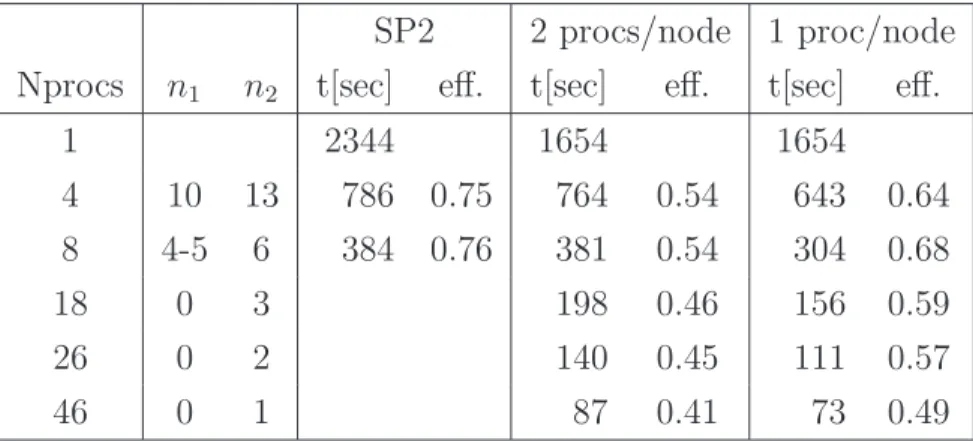
3.1 Runtime and scaling efficiency of the spectral code. . . 56 4.1 Orbital parameters of the innermost stable circular orbit for

equal-mass spinning holes . . . 79 4.2 Summary of common apparent horizon searches . . . 81 5.1 ISCO parameters for different mass-ratios obtained with the

effec-tive potential method. . . 98 6.1 Solutions of different decompositions for two black holes at rest . . 127 6.2 Initial-data sets generated by different decompositions for binary

black holes with orbital angular momentum . . . 131 6.3 Solutions of ConfTT for different radii of the excised spheres, rexc . 136

6.4 Solutions of CTS as a function of radius of excised spheres, rexc.

Different choices of the lapse ˜α and boundary conditions for ψ at the excised spheres are explored. . . 137 7.1 Spherically symmetric single black hole solutions . . . 156 7.2 Parameters for equal mass binary black hole solutions constructed

with the quasi-equilibrium method. . . 175

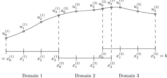
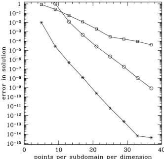
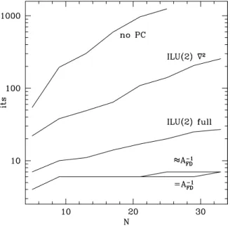
2.1 Setup for conformal thin sandwich equations . . . 9 3.1 Illustration of matching with three subdomains in one dimension . 37 3.2 Domain decomposition for Laplace equation in a square . . . 45 3.3 Convergence of solution of Laplace equation in a square . . . 46 3.4 Iteration count of the linear solver for different types of

precondi-tioning . . . 47 3.5 Domain decomposition for the domain R

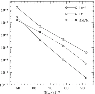
3 _{with two excised spheres 49} 3.6 Convergence of solution of Eqs. (3.52)-(3.55) for equal-sized holes . 50 3.7 Convergence of solution of Eqs. (3.52)-(3.55) for widely separated,

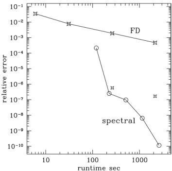
unequal sized holes . . . 52 3.8 Comparison of runtime vs. achieved accuracy for the new spectral

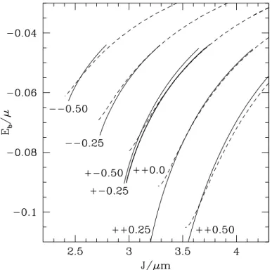
solver and the Cad´ez code . . . 54 3.9 Convergence of solution to coupled PDEs (3.58) and (3.59) . . . 58 4.1 Sequences of quasi-circular orbits for different spin configurations:

binding energyEb/µ vs. angular momentum J/µm . . . 72

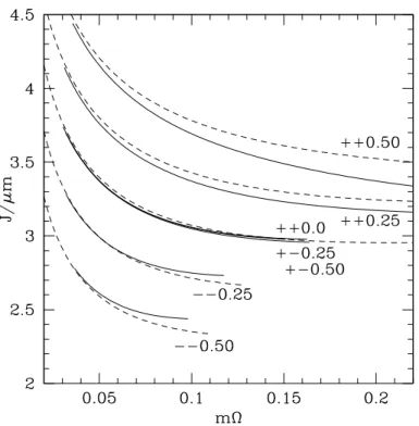
4.2 Sequences of quasi-circular orbits for different spin configurations: binding energyEb/µ vs. orbital angular frequency mΩ . . . 73

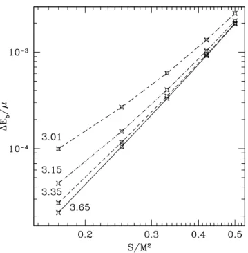
4.3 Sequences of quasi-circular orbits for different spin configurations: angular momentum J/µm vs. orbital angular frequency mΩ . . . . 74 4.4 Difference in binding energy ∆Eb/µ between +− sequences and

non-rotating sequence as a function of spin of the +_{−sequence for}

fixed angular momentum J/µm . . . 75 4.5 Constant J/µm contours of the effective potential Eb/µ as a

func-tion of separafunc-tion ℓ/mfor various spin configurations . . . 77 4.6 Enlargement of the++_{0.17 sequence of Fig. 4.5 . . . . 79}

4.7 Values of several physical parameters at the ISCO of the ++ _and −−sequences. . . 80 4.8 Shapes of the common apparent horizons for different spin

config-urations . . . 82 4.9 Illustration of the effects of a systematic underestimation of Eb/µ 85

4.10 Residual of the minimization in the apparent horizon finder as a function of expansion order L . . . 90 5.1 Sequences of quasi-circular orbits for different mass-ratios obtained

with inversion symmetric Bowen-York initial data (small L/µm) . . 94 5.2 Sequences of quasi-circular orbits for different mass-ratios obtained

with inversion symmetric Bowen-York initial data. . . 95 5.3 Sequences of quasi-circular orbits for different mass-ratios obtained

with inversion symmetric Bowen-York initial data (largeL/µm) . . 96 5.4 ISCO’s for different mass-ratios obtained with inversion symmetric

Bowen-York initial data. . . 97 xiii

6.3 Testing the solver for the conformal TT decomposition . . . 119 6.4 Testing the solver for the physical TT decomposition with domain

decomposition . . . 120 6.5 Testing thin sandwich decomposition with apparent horizon searches123 6.6 Convergence of binary black hole solution with conformal TT

de-composition . . . 124 6.7 The conformal factor ψ along the axis connecting the holes for

several decompositions . . . 126 6.8 Black holes at rest: Contour plots of the conformal factor ψ for

ConfTT and CTS-add . . . 128 6.9 Plots ofψ andVx _{along the positivex-axis for ConfTT for different}

radii rexc= 2M, M,0.5M,0.2M . . . 135

6.10 Apparent horizons for ConfTT with different radii of excised spheres135 6.11 Cuts through ψ and βx _{for CTS-mult for different radiir}

exc . . . . 138

6.12 Apparent horizons for CTS with ˜α = NANB and inner boundary

condition dψ/dr= 0 . . . 139 7.1 Inner boundary for quasi-equilibrium boundary conditions . . . 146 7.2 Solving the quasi-equilibrium equations (7.28) on an

Eddington-Finkelstein slice . . . 154 7.3 Minimum of N as a function of the coefficient Ξ in the modified

lapse boundary condition. . . 161 7.4 Quasi-equilibrium binary black hole initial data sets on

Eddington-Finkelstein slices: dependence on Ω . . . 164 7.5 Quasi-equilibrium binary black hole initial data set on an

Eddington-Finkelstein slice . . . 165 7.6 Quasi-equilibrium binary black hole initial data sets on maximal

slices: Dependence on Ω. . . 166 7.7 Quasi-equilibrium binary black hole initial data set on an maximal

slice . . . 167 7.8 Quasi-equilibrium method in the test-mass limit: Various

quanti-ties as a function of the mass-ratio . . . 170 7.9 ∂tlnψ and shift βi for initial data sets with mass-ratio 16. . . 171

7.10 ∂tlnψ and shift βi for a single boosted black hole. . . 173

7.11 Testing the quasi-equilibrium equations and the lapse quasi-equilibrium condition on an Eddington-Finkelstein slice. . . 182 7.12 Convergence of selected terms of the lapse boundary condition. . . 183 8.1 Domain decomposition used for elliptic solves in fullR3_{. . . 192} 8.2 Constraint violation of linear gravitational wave in flat background. 193 8.3 ADM energy of an ingoing Gaussian pulse in flat space. . . 193 8.4 Cuts through the equatorial plane of theA= 0.3 data set of Fig. 8.3.194

8.6 Apparent horizon mass during an evolution of a perturbed black hole spacetime. . . 196

Introduction

General relativity is entering a very exciting phase with the commissioning of several gravitational wave detectors. The detection of gravitational waves serves two main purposes. It allows fundamental tests of the theory of general relativity in the genuinely nonlinear regime, and it advances astrophysics by opening a new observational window which can be used for detailed studies of individual sources and for source statistics.

One prime target for gravitational wave detectors is binary systems of compact objects, black holes or neutron stars. Such a binary system emits energy and an-gular momentum through gravitational radiation, so that the orbital separation slowly decreases. The best-known example is the “Hulse-Taylor” pulsar. Gravita-tional radiation tends to circularize orbits, leading to almost circular orbits during late inspiral. For binary black holes, the orbits become unstable at some small separation, the so-called innermost stable circular orbit, where the slow adiabatic inspiral changes to a dynamical plunge. The two black holes merge and form a single distorted black hole, which subsequently settles down to a stationary black hole by emission of further gravitational radiation during the ring-down phase.

Early inspiral can be treated with post-Newtonian expansion, and the late ring-down phase is accessible to perturbation theory. It is generally believed, however, that the late inspiral and the dynamical merger can only be treated with a full numerical evolution of Einstein’s equations, which is therefore essential to obtain the complete waveform of a binary black hole coalescence. The knowledge of the wave-form is essential for finding the gravitational wave signal amidst the detector noise in the first place (cross-correlation with known waveform templates greatly enhances the sensitivity of the detectors), and to extract as much information as possible about identified events. One needs to know the prediction of general relativity, especially in the nonlinear regime, to compare it to the observations.

Besides the importance of numerical relativity for the experiments, it also en-compasses the intellectual challenge of solving the two-body problem. While the Newtonian two-body problem is treated completely in freshman mechanics, the general relativistic analogue, the binary black hole, is still unsolved.

Any evolution must start with initial data. For an evolution of Einstein’s equations, setting initial data is difficult for several reasons:

First, the initial data must satisfy constraints, analogous to the divergence equations of electrodynamics,

∇ ·E~ = 4πρ,

∇ ·B~ = 0. (1.1)

Any initial data E~ and B~ for an evolution of Maxwell’s equations must satisfy Eqs. (1.1). Similarly, initial data for Einstein’s equations must satisfy constraint equations, which are, however, much more complicated than Eqs.(1.1). Thus, one is faced with the mathematicaltask of finding a well-defined method to construct solutions to the constraint equations of general relativity. This problem has been an active research area for almost sixty years.

Second, formalisms to solve the constraint equations usually lead to sets of coupled nonlinear elliptic partial differential equations in three dimensions, often on a computational domain which has excised regions. Solving such a set of equations is a formidablenumerical task.

Third, the mathematical formalisms to construct initial data sets leave an enor-mous amount of freedom. Some ten functions of space can be freely specified. These functions are generally called the “free data.” Hence, even with an elliptic solver in hand, one is faced with the physical question of which initial data sets from the infinite parameter space are astrophysically relevant. Initial data rep-resenting a binary black hole, for example, must contain two black holes which, if evolved, actually move on almost circular orbits. Furthermore, the initial data should not contain unphysical gravitational radiation; ideally, however, it should contain the outgoing gravitational radiation emitted during the preceding inspiral.

This thesis attempts to contribute to each of these three aspects.

In chapter 2 we present the latest formalisms to decompose the constraint equations. We outline the main ideas of the two relevant papers by York [1] and Pfeiffer & York [2]. We also comment on various issues which are important in general, and/or will arise in later chapters of the thesis.

Chapter 3 develops a new code to solve elliptic partial differential equations, a pseudospectral collocation method with domain decomposition. The exponential convergence of spectral methods for smooth functions allows very accurate solu-tions. The domain decomposition makes it possible to handle complex topologies, e.g. with excised spheres, and to distribute grid-points to improve accuracy. Last, but not least, the code is designed to be modular and very flexible, making it easy to explore different partial differential equations or different boundary conditions.

All three of these characteristics have proved to be essential for the present work. The remaining chapters of the thesis explore initial data sets with a variety of approaches.

Chapters 4 and 5 compute binary black holes in circular orbits for spinning black holes (chapter 4) and unequal mass black holes (chapter 5). We employ the effective potential method based on conformally flat inversion-symmetric Bowen-York initial data. The most important result from these two chapters is, perhaps, that this method is not optimal. In the test-mass limit one can assess the quality of many of the approximations used, and one can compare the numerical method against an analytical result. This makes it possible to pin-point the problem of the numerical method with some confidence. We argue that the choice of the so-called extrinsic curvature, namely the Bowen-York extrinsic curvature is problematic. In the calculation for spinning equal-mass black holes, the symptoms of failure are easily seen (disappearance of the ISCO for corotating holes with moderate spin, and an unphysical (spin)4_{-effect); however, the causes are less clear due to the large} number of assumptions made.

As there is widespread belief that the approximation of conformal flatness lim-its the physical relevance of initial data sets (for example, binary compact objects are not conformally flat at second post-Newtonian order), we relax this approxi-mation in chapter 6. We compute data sets that are not conformally flat using different mathematical formalisms and different choices for the free data. We then compare these data sets with each other. For the data sets considered, we do not find evidence that the non-conformally flat initial data sets are superior. We find, however, a sensitive dependence on the extrinsic curvature. Two different choices for the extrinsic curvature (“ConfTT” and “mConfTT” in the language of chapter 6), which are equally well motivated, result in drastically different initial data sets. While the approximation of conformal flatness will have to be addressed eventually, especially for rotating black holes, I believe that it is currently not the limiting factor.

One formalism to solve the constraints, the conformal thin sandwich method, does not require specification of an extrinsic curvature. It thus might well avoid ambiguities like the one we just mentioned. A special case of this method was recently used in another approach to compute quasi-circular orbits of binary black holes, thehelical Killing vector approximation, which has been generalized by Cook to the quasi-equilibrium method. Chapter 7 describes this method and examines

the resulting set of partial differential equations and boundary conditions. We compute single black hole spacetimes, and binary black holes in circular orbits with two different choices of the remaining free data. We further examine the test-mass limit as well as the limit of widely separated black holes. In both limits, we show that the current choices for the remaining free data are unsatisfactory. We also discuss a proposal for a lapse boundary condition put forth by Cook, and explain how to perform a certain extrapolation required to use these data sets as initial data for evolutions.

Chapter 8, finally, changes gear again and describes a new and general way to construct spacetimes with superposed gravitational radiation. The attractive feature of this method is that it admits a simple physical interpretation of the wave, and one can specify directly the radial shape and angular dependence of the wave, as well as the direction of propagation. As examples, I construct spacetimes without a black hole containing ingoing spherical pulses of varying amplitude, as well as spacetimes containing one black hole surrounded by a similar pulse. The amplitude of these pulses can be very large; in extreme cases most of the energy contained in the spacetime is outside the black hole. In this chapter, we solve the conformal thin sandwich equations on very general, nonflat conformal manifolds; the fact that this is easily possible highlights the robustness of the conformal thin sandwich formalism and of the spectral elliptic solver.

During the work described in this thesis, I have also improved an apparent horizon finder that was developed at Cornell a few years ago. Details can be found in sections 4.6 and 6.4.2.

The primary goal of this thesis is to construct initial datafor evolutions. Indeed, data sets from chapters 6, 7 and 8 are used in evolutions by the numerical relativity group at Cornell. As the results from evolutions are preliminary so far, I restrict discussion here to the initial data sets.

The initial value problem of general

relativity

Numerical relativity attempts to construct a spacetime with metric(4)_g

µν(µ, ν, . . .=

0,1,2,3) which satisfies Einstein’s equations,

Gµν = 8πGTµν. (2.1)

Within the standard 3+1 decomposition [3, 4] of Einstein’s equations, the first step is to single out a time coordinate “t” by foliating the spacetime with spacelike

t=const. hypersurfaces. Each such hypersurface surface has a future pointing unit-normalnµ_{, induced metricg}

µν =(4)gµν+nµnν and extrinsic curvature Kµν =

−1

2Lngµν. We use the label t of the hypersurfaces as one coordinate and choose 3-dimensional coordinates xi _{within each hypersurface (i, j, . . .= 1,2,3). The three}

dimensional metricgµν andKµν are purely spatial tensors; we denote their spatial

components by gij and Kij. The spacetime metric can be written as

ds2 =₋N2dt+gij dxi+βidt

dxj+βjdt, (2.2)

where N and βi _{denote the lapse function and shift vector, respectively. N}

mea-sures the proper separation between neighboring hypersurfaces along the surface normals and βi _{determines how the coordinate labels move between}

hypersur-faces: Points along the integral curves of the “time”–vectortµ _=Nnµ_+βµ _(where

βµ_{= [0, β}i_{]), have the same spatial coordinates x}i_.

Einstein’s equations (2.1) decompose into evolution equations and constraint equations for the quantities gij and Kij.

The evolution equations determine how gij and Kij are related between

neigh-boring hypersurfaces,

∂tgij =−2NKij +∇iβj+∇jβi (2.3)

∂tKij =N Rij −2KikKjk+KKij−8πGSij+ 4πGgij(S−ρ)

− ∇i∇jN +βk∇kKij+Kik∇jβk+Kkj∇iβk. (2.4)

Here, _∇i and R are the covariant derivative and the scalar curvature (trace of

the Ricci tensor) of gij, respectively, K =Kijgij is the trace of Kij, the so-called

mean curvature, ρand Sij are matter density and stress tensor1, respectively, and

S=Sijgij denotes the trace ofSij.

The constraint equations are conditions within each hypersurface alone, ensur-ing that the three-dimensional surface can be embedded into the four-dimensional spacetime:

R+K2−KijKij = 16πGρ, (2.5)

∇j Kij −gijK

= 8πGji, (2.6)

withji_{denoting the matter momentum density. Equation (2.5) is called the}

Hamil-tonian constraint, and Eq. (2.6) is the momentum constraint.

Cauchy initial data for Einstein’s equations consists of (gij, Kij) on one

hyper-surface satisfying the constraint equations (2.5) and (2.6). After choosing lapse and shift (which are arbitrary — they merely choose a specific coordinate system), Eqs. (2.3) and (2.4) determine (gij, Kij) at later times. Analytically, the constraints

equations are preserved under the evolution. (In practice during numerical evolu-tion of Eqs. (2.3) and (2.4), or any other formulaevolu-tion of Einstein’s equaevolu-tions, many problems arise. However, we will focus on the initial value problem here.)

The constraints (2.5) and (2.6) restrict four of the twelve degrees of freedom of (gij, Kij). As these equations are not of any standard mathematical form, it is not

obvious which four degrees of freedom are restricted. Hence, finding any solutions is not trivial, and it is even harder to construct specific solutions that represent certain astrophysically relevant situations like a binary black hole.

Work on solving the constraint equation dates back almost sixty years to Lich-nerowicz [5], but today’s picture emerged only very recently in work due to York [1, 2]. I will describe two general approaches to solving the constraint equations. The first one is based on the metric and its time-derivative on a hypersurface, whereas the second one rests on the metric and the extrinsic curvature. Since the extrinsic curvature is essentially the canonical momentum of the metric (e.g. [6]), the latter approach belongs to the Hamiltonian picture of mechanics whereas the former one is in the spirit of Lagrangian mechanics.

1_{In later chapters of this thesis, we deal exclusively with vacuum spacetimes for} which all matter terms vanish; we include them in this chapter for completeness.

2.1

Preliminaries

Both pictures make use of a conformal transformation on the metric,

gij =ψ4g˜ij (2.7)

with strictly positiveconformal factorψ. ˜gij is referred to as theconformal metric.

From (2.7) it follows that the Christoffel symbols of the physical and conformal metrics are related by

Γi_jk = ˜Γi_jk+ 2ψ−1 δ_ji∂kψ+δki∂jψ−˜gjk˜gil∂lψ

. (2.8)

Equation (2.8) implies that the scalar curvatures of gij and ˜gij are related by

R=ψ−4R˜−8ψ−5∇˜2_{ψ. (2.9)}

Equations (2.7)–(2.9) were already known to Eisenhart [7]. Furthermore, for any symmetric tracefree tensor ˜Sij_,

∇j

ψ−10S˜ij=ψ−10_∇˜jS˜ij, (2.10)

where ˜_∇is the covariant derivative of ˜gij. Lichnerowicz [5] used Eqs. (2.7) to (2.10)

to treat the initial value problem on maximal slices,K = 0. For non-maximal slices, we split the extrinsic curvature into trace and tracefree parts,

Kij =Aij + 1

3g

ij_{K. (2.11)}

With (2.9) and (2.11), the Hamiltonian constraint (2.5) becomes ˜ ∇2_ψ− 1 8ψR˜− 1 12ψ 5_K2₊1 8ψ 5_A ijAij + 2πGψ5ρ= 0, (2.12)

a quasi-linear Laplace equation for ψ. Local uniqueness proofs of equations like (2.12) usually linearize around an (assumed) solution, and then use the maximum principle to conclude that “zero” is the only solution of the linearized equation. However, the signs of the last two terms of (2.12) are such that the maximum principle cannot be applied. Consequently, it is not immediately guaranteed that Eq. (2.12) has unique (or even locally unique) solutions2_{. The term proportional} 2_{As a physical illustration of possible problems, consider the matter term} 2πGψ5_{ρ, a source which pushes ψ to larger values. The physical volume element,}

dV =√gd3_x=ψ6√_˜gd3_{x, expands asψ becomes larger. With physicalmatter} en-ergy density ρ given, the total matter content will grow like ψ6 _{and will therefore} becomestronger, pushing ψ to even larger values. Beyond some critical value ofρ, a “run-away” might set in pushing ψ to infinity. Indeed I observed this behavior while solving the constraint equations coupled to a scalar field.

to AijAij will be dealt with later; for the matter terms we follow York [4] and

introduce conformally scaled source terms:

ji =ψ−10˜i, (2.13)

ρ=ψ−8ρ.˜ (2.14)

The scaling for ji _{makes the momentum constraint below somewhat nicer; the}

scalings of ρ and ji _{are tied together such that the dominant energy condition}

preserves sign:

ρ2−gijjijj =ψ−16 ρ˜2−˜gij˜i˜j

≥0. (2.15)

The scaling of ρ, Eq. (2.14) modifies the matter term in (2.12) to 2πGψ−3_ρ˜with negative semi-definite linearization for ˜ρ≥0.

The decomposition of Kij into trace and tracefree part, Eq. (2.11), turns the

momentum constraint (2.6) into

∇jAij −

2 3∇

i_{K = 8πGj}i_{. (2.16)}

For time-symmetric vacuum spacetimes (where Aij_=K=ji_{= 0 solve the}

momen-tum constraint (2.16) trivially), only the first two terms of (2.12) remain. This simplified equation was used in beautiful early work on vacuum spacetimes, for example a positivity of energy proof by Brill [8] and construction of multi black hole spacetimes by Misner [9] and Brill & Lindquist [10].

The conformal transformation (2.7) implies one additional, very simple, con-formal scaling relation. The longitudinal operator [11, 12, 13]

(LV)ij _{≡ ∇}iVj +_∇jVi₋ 2 3g ij ∇kVk, (2.17) satisfies [12] (_LV)ij _=ψ−4_(˜ LV)ij_{. (2.18)}

Here (˜LV)ij _{is given by the same formula (2.17) but with quantities associated}

with the conformal metric ˜gij. (In fluid dynamics (LV)ij is twice the shear of the

velocity fieldVi_{). In ddimensions, the factor 2/3 in Eq. (2.17) is replaced by 2/d;}

Eq. (2.18) holds for alld.

2.2

Conformal thin sandwich formalism

We now derive a formalism to solve the constraint equations [1] which deals with the conformal metric and its time derivative. This formalism thus represents the

Lagrangian viewpoint. Figure 2.1 illustrates the basic setup; we deal with two

hypersurfaces separated by the infinitesimal δt (thus the name “thin sandwich”), and connected by the lapse N and the shift βi. The mean curvature of each hypersurface is K and K + ˙Kδt, respectively. The metric is split into conformal factor and conformal metric; on the first hypersurface, this is simply Eq. (2.7). On the second hypersurface, the conformal factor and the conformal metric will both be different from their values on the first hypersurface. The split into conformal factor and conformal metric is not unique and is synchronized between the two surfaces by requiring that the conformal metrics on both hypersurfaces have the same determinant to first order in δt. The variation of the determinant of ˜gij is

given by

δg˜= ˜gg˜ijδg˜ij = ˜gg˜iju˜ijδt (2.19)

(the first identity holds for any square matrix), so that ˜uij =∂tg˜ij must be traceless.

On the first hypersurface the Hamiltonian constraint will eventually determineψ. Besides the relationships indicated in Figure 2.1, the conformal thin sandwich formalism rests on the nontrivial scaling behavior of the lapse function:

N =ψ6N .˜ (2.20)

The scaling (2.20) appears in a bewildering variety of contexts (see references in [1, 2]). For example, studies ofhyperbolicevolution systems for Einsteins equations (e.g. [14, 15]) find that hyperbolicity requires that the lapse anti-density (“densi-tized lapse”) α _≡ g−1/2_{N is freely specifiable, not N directly (recall} √_{g =ψ}6√_g˜, so thatαis essentially equivalent to ˜N). The scaling (2.20) is crucial in the present context as well, cf. Eq. (2.26) below.

. ... . ... . . . . . ... . . . . . . . . . . . . . . . . Nn δtˆ . . . . . . . . . . . . . . . . . . . . . . . . . . . . . . . . . . . . . . . . . . . . . . . . . . . . . . . . . . . . . . . . . . . ... ... β δt... . . . . . . . . . . ... t δt= (Nnˆ+β)δt . . . . . . . . . . . . . . . . . . . . . . . . . . . . . . . . . . . . . . . . . . . . . . . . . . . . . . . . . . . . . . . . . . . . . . . . . . . . . . . ... . ... . . ... . . . ... ˜ gij, ψ ˜ gij + ˜uijδt ψ + ˙ψ δt K K+ ˙K δt

Substitution of Eq. (2.7) into the evolution equation for the metric, Eq. (2.3), yields

4ψ4(∂tlnψ)˜gij +ψ4∂tg˜ij =−2NKij +∇iβj +∇jβi. (2.21)

Since ∂t˜gij = ˜uij is traceless, the left hand side of Eq. (2.21) is already split into

trace and tracefree parts. Splitting the right hand side, too, gives

ψ4u˜ij =−2NAij + (Lβ)ij (2.22) and ∂tlnψ =− 1 6NK+ 1 6∇kβ k_{. (2.23)}

(The factor ψ4 _{in (2.23) cancels because the trace is performed with the physical} inverse metric gij _{= ψ}−4_˜gij_{). Equation (2.22) is the tracefree piece of ∂}

tgij, thus foruij ≡ψ4u˜ij, uij =∂tgij − 1 3gijg kl_∂ tgkl. (2.24)

Now solve Eq. (2.22) forAij_,

Aij = 1

2N (Lβ)

ij _−uij_{, (2.25)}

and rewrite with conformal quantities [using (2.20), (2.18) anduij _=ψ−4_u˜ij_]:

Aij = 1 2ψ6_N˜ ψ−4(˜Lβ)ij ₋ψ−4u˜ij=ψ−10 1 2 ˜N (˜Lβ)ij ₋u˜ij_≡ψ−10A˜ij (2.26) with the conformal tracefree extrinsic curvature

˜

Aij = 1

2 ˜N

(˜Lβ)ij ₋u˜ij. (2.27)

Equation (2.26) shows that the formula forAij _{is form invariant under conformal}

transformations; this hinges on the scaling of N in Eq. (2.20). Substitution of Eq. (2.26) into the momentum constraint (2.16) and application of Eq. (2.10) yields ˜ ∇j 1 2 ˜N(˜Lβ) ij −∇˜j 1 2 ˜Nu˜ ij − 2₃ψ6_∇˜iK = 8πG˜i, (2.28) whereas Eq. (2.26) modifies the Hamiltonian constraint (2.12) to3

˜ ∇2_ψ−1 8ψR˜− 1 12ψ 5_K2₊ 1 8ψ −7_A˜ ijA˜ij =−2πGψ−3ρ.˜ (2.29)

3_{Indices on conformal quantities are raised and lowered with the conformal} metric, for example

Equations (2.28) and (2.29) constitute elliptic equations for βi _{and ψ. We thus}

find the following procedure to compute a valid initial data set:

A. Choose the free data

(˜gij, u˜ij, K, N˜) (2.30)

(and matter terms if applicable).

B. Solve Eqs. (2.28) and (2.29) for βi _{and ψ.}

C. Assemble gij =ψ4g˜ij and Kij =ψ−10A˜ij +1₃gijK.

The conformal thin sandwich formalism does not involve transverse-traceless decompositions, and is therefore somewhat more convenient than the extrinsic curvature decomposition discussed in section 2.3. We now comment on several issues related to the conformal thin sandwich formalism.

2.2.1

Fixing ˜

N

via ˙

K

The free data so far is given by (2.30). Whereas ˜gij and ˜uij = ∂tg˜ij constitute a

“variable & velocity pair” (q,q˙) in the spirit of Lagrangian mechanics, the remain-ing free data does not.

As we show starting with Eq. (2.32) below, specification of ∂tK = ˙K fixes ˜N

through an elliptic equation. If we take ˙K as the “free” quantity instead of ˜N, then the free data for the conformal thin sandwich formalism becomes

(˜gij, u˜ij, K, K˙) (2.31)

plus matter terms if applicable. These free data consists completely of (q,q˙) pairs as appropriate for a Lagrangian viewpoint. The free data (2.31) is also useful practically for computations of quasi-equilibrium initial data sets in chapter 7. In quasi-equilibrium, ˙K = 0 is a natural and simple choice, whereas it is not obvious at all which conformal lapse ˜N one should use. In particular, ˜N will depend on the slicing of the spacetime.

We now derive the elliptic equation for ˜N (see, e.g., [16]). The trace of the evolution equation forKij, Eq. (2.4), gives after some calculations

∂tK−βk∂kK =N R+K2+ 4πG(S−3ρ)

Elimination of R with the Hamiltonian constraint (2.5) yields

∇2N ₋N KijKij + 4πG(S+ρ)

=₋∂tK+βk∂kK. (2.33)

Rewriting the Laplace operator with conformal derivatives,

∇2_{N =} 1 √_g∂i √ggij∂jN = ψ− 6 √ ˜ g∂i ψ2pg˜g˜ij∂jN =ψ−4∇˜2_{N + 2ψ}−4_∇˜ ilnψ∇˜iN,

together with Eqs. (2.20) and (2.29) gives ˜ ∇2N˜ + 14 ˜_∇ilnψ_∇˜iN˜ + ˜N 3 4R˜+ 1 6ψ 4_K2 −7 4ψ −8_A˜ ijA˜ij (2.34) +42 ˜_∇ilnψ∇˜ilnψ−4πGψ4(S+4ρ) =₋ψ−2 ∂tK−βk∂kK ,

which can also be rewritten as ˜ ∇2( ˜Nψ7)₋( ˜N ψ7) 1 8R˜+ 5 12ψ 4_K2₊7 8ψ −8_A˜ ijA˜ij + 2πGψ4(ρ+ 2S) (2.35) =₋ψ5 ∂tK−βk∂kK .

Equation (2.34) determines the freely specifiable ˜N directly, whereas Eq. (2.35) is shorter and therefore computationally somewhat more convenient.

We now have a system of five coupled partial differential equations, (2.28), (2.29) and (2.34) [or (2.35)] with freely specifiable data (2.31).

2.2.2

Invariance to conformal transformations of the free

data

Assume we specify free data (2.30), solve the conformal thin sandwich equations for conformal factorψand shiftβi_{, and assemble the physical initial data (g}

ij, Kij).

We now pick a function Ψ > 0, and perform a conformal transformation on the free data (2.30) by setting

˜

g_ij′ = Ψ−4g˜ij, u˜′ij = Ψ4u˜ij, K′ =K, N˜′ = Ψ−6N,˜ (2.36)

plus the scalings ˜ρ′ = Ψ8_{ρ,˜ ˜}′i _{= Ψ}10_˜i _{for matter terms if applicable. These free}

βi _{are the solutions to the conformal thin sandwich equations using the original}

free data) lead to the samephysical initial data (gij, Kij):

g_ij′ =ψ′4 _˜g′ ij =ψ4˜gij =gij, (2.37) A′ij =ψ′ −10 1 2 ˜N′ ˜ L′β′ij ₋u˜′ij = (Ψψ)−10 1 2Ψ−6_N˜ Ψ4 _L˜βij ₋Ψ4u˜ij=Aij. (2.38) Here, we used Eqs. (2.7), (2.18) and (2.26). Adding the trace of the extrinsic curvature to (2.38) is trivial.

We thus find that only the conformal equivalence class of ˜gij is relevant for

the physical solution. This is a very desirable property; we introduced ˜gij as a

conformalmetric, so its overall scaling should not matter. Fixing ˜Nby specification of ˙K preserves this invariance, as the ˙K-equation, (2.34), is derived from physical

quantities in the first place.

The extrinsic curvature decomposition introduced in the next section is also invariant under conformal transformations of the free data. We note that invariance under conformal transformations of the free data is not trivial; earlier variants of the constraint decompositions did not possess it, giving rise to ambiguities in the free data [17].

2.2.3

Gauge degrees of freedom

The physical initial data (gij, Kij) has twelve degrees of freedom4. It is constrained

by four constraint equations, so there should be eight degrees of freedom in the freely specifiable data. However, taking into account that only the conformal equivalence class of ˜gij is relevant and that ˜uij is traceless, one sees that the free

data (2.30) or (2.31) consists of twelve quantities, not eight. To examine this further, we consider the substitutions

˜

uij → u˜ij+ (˜LW)ij,

βi _→ βi+Wi. (2.39)

The vectorWi_{disappears from Eqs. (2.27)–(2.29), therefore the substitution (2.39)}

will not change the physical initial data set (gij, Kij); it merely tilts the time-axis

4_{Matter just adds four additional degrees of freedom in ˜ρand ˜}i_{which determine}

the four physical matter variables ρ and ji_{. It therefore does not influence the}

and changes the coordinate labels on the second hypersurface. Thus, ˜uij contains

three gauge degrees of freedom associated with the shift. (Wi _{enters into Eq. (2.34)}

as an advection term, though, because∂tK is the derivativealong the time-vector,

which of course must be sensitive to the directionof the time-vector).

The fourth “missing” degree of freedom is hidden in the lapse function ˜N: One can construct every possible initial data set (gij, Kij) with any (non-pathologic)

choice of ˜N. This is easiest seen by going backward from the physical initial data (gij, Kij) (satisfying the constraints) to the free data. Given (gij, Kij) and any

˜

N and βi_{, there exists free data such that solving the conformal thin sandwich}

equations gives back the original physical initial data set (gij, Kij). These free

data are:

˜

gij =gij, u˜ij = (Lβ)ij−2 ˜NAij, K =Kijgij (2.40)

plus the given ˜N (whatever it may be). With these choices for the free data,

ψ _≡1 and the givenβi _{will reconstruct the physical spacetime (g}

ij, Kij) as can be

seen from Eqs. (2.7) and (2.26). Therefore, ψ _≡1 and the given βi _{will solve the}

conformal thin sandwich equations (2.28) and (2.29).

The fact that we were free to choose βi _{reflects again the gauge-symmetry}

illustrated in Eq. (2.39), but in addition, we showed that the choice of ˜N does not restrict the set of “achievable” initial data sets.

Note that the physical initial data contain further gauge freedom: Covariance under spatial transformations implies thatgij (and ˜gij) contain three gauge degrees

of freedom associated with the choice of coordinates. Furthermore, K can be interpreted as time [18], fixing the temporal gauge. Thus, an initial data set has only four physical degrees of freedom—in perturbed flat space they are simply the two polarizations of gravitational waves.

2.2.4

Implications for an evolution of the initial data

During the solution of the conformal thin sandwich equations, one finds a shiftβi

and a lapse N. If one uses this lapse and shift in a subsequent evolution of the initial data (gij, Kij) —recall that any lapse and shift can be used— then Eq. (2.24)

implies thatinitially,

∂tgij −

1 3gijg

kl_∂

tgkl =ψ4u˜ij. (2.41)

The freely specifiable piece ˜uij thus directly controls the tracefree part of the

the evolution will initially have ∂tK = ˙K, too. Finally, from (2.23), we find ∂tlnψ = 1 6 ∇kβ k_−NK = 1 6∇˜kβ k_+βk_∂ klnψ− 1 6ψ 6_{NK.˜ (2.42)}

This is essentially the trace of ∂tgij.

Since we have been very successful so far with specification of time-derivatives (∂tg˜ij and ∂tK), one might be tempted to turn (2.42) around and use it as the

definitionofK in terms of∂tlnψ. This idea certainly comes to mind when looking

for quasi-equilibrium solutions, for which as many time-derivatives as possible should vanish. From (2.42) we find

K = 1 ψ6_N˜ ˜ ∇kβk−6 ∂t−βk∂k lnψ. (2.43)

We see that K contains first derivatives of the shift. The gradient of K enters the momentum constraint (2.28), therefore (2.43) will modify the second derivatives of the elliptic operator in (2.28). The terms containing second derivatives of βi _in

Eq. (2.28) become ˜ ∇j 1 2 ˜N(˜Lβ) ij − 2₃ψ6_∇˜i 1 ψ6_N˜ ˜ ∇kβk . (2.44)

Using the product rule, discarding first derivatives of βi_{, and using the definition}

of L, Eq. (2.17), we find 1 2 ˜N ˜ ∇j∇˜jβi+ ˜∇j∇˜iβj −2 ˜∇i∇˜kβk . (2.45)

Commuting the derivatives in the second term yields a term proportional to the Riemann tensor, which is discarded as it contains no derivatives ofβi _{at all. After}

multiplication by ˜N, the highest-order derivatives of βi _{in the momentum}

con-straint become

∂j∂jβi−∂i∂kβk. (2.46)

This operator is non-invertible; for example it maps the functions

fj(xl) =kjexp i klxl

(2.47) to zero for any choice of the wave-vector ki_{. Thus, the attempt to fixK via (2.43)}

In practice I encountered a consequence of this fact when constructing quasi-equilibrium slices of spherically symmetric spacetimes. For that case, we show in section 7.4.2 that the conformal thin sandwich equations with ˜uij = 0 and ˙K = 0

(and appropriate boundary conditions) are so successful in picking out the time-like Killing vector that for any choice of K, the solution satisfies ∂tlnψ = 0. If

∂tlnψ = 0 for any choice of K, then ∂tlnψ = 0 obviously cannot determine a

unique K.

In contrast to the trace-free part (2.41) we can not easily control ∂tlnψ by

choices of the free data. We can only evaluate (2.42) after solving the conformal thin sandwich equations.

2.3

Extrinsic curvature decomposition

The second method to construct solutions of the constraint equations if based on a decomposition of the extrinsic curvature. Early variants of this approach [19, 4] have been available for almost thirty years, but the final version was developed only very recently [2]. We will make use of the equations and results from section 2.1, in particular, we use a conformal metric, gij = ψ4˜gij, and split the extrinsic

curvature into trace and trace-free parts, Kij _=Aij _{+ 1/3g}ij_{K, cf. Eqs. (2.7) and}

(2.11).

We start with a weighted transverse traceless decomposition of Aij_,

Aij =Aij_{T T} + 1

σ(LV)

ij

. (2.48)

Here, Aij_{T T} is transverse, _∇jAT Tij = 0, and traceless, gijAijT T = 0, and σ is a strictly

positive and bounded function. Appearance of the weight functionσ is a key point in the extrinsic curvature formulation; its inclusion is the major improvement of [2] over the older variants.

Given a symmetric tracefree tensor like Aij_{, the decomposition (2.48) can be}

obtained by taking the divergence of Eq. (2.48),

∇jAij =∇j

σ−1(LV)ij. (2.49)

The right hand side, _∇j[σ−1(L.)ij], is a well-behaved elliptic operator in

diver-gence form, so no problem should arise when solving (2.49) for Vi_{. Substitution}

of the solutionVi _{back into (2.48) yields the transverse traceless partA}ij

presence of boundaries, Eq. (2.49) requires boundary conditions which will influ-ence the solutionVi _{and the decomposition (2.48). For closed manifolds, existence}

and uniqueness of the decomposition (2.48) for the caseσ ≡1 was shown in [13]. We now conformally scale the quantities on the right hand side of (2.48) with the goal of rewriting the momentum constraint in conformal space.

First, we set

Aij_{T T} ≡ψ−10A˜ij_{T T}. (2.50)

Equation (2.10) ensures that ˜Aij_{T T} is transverse with respect to ˜gij if and only if

Aij_{T T} is transverse with respect to the physical metric gij.

Because of Eq. (2.18), and because Lis the conformal Killing operator, we will not scale the vector Vi_.

The conformal scaling of the weight function is given by

σ=ψ6σ.˜ (2.51)

The most immediate reason for this scaling is that it allows Eq. (2.52) below; several more reasons will be mentioned in the sequel.

Using the scaling relations (2.18), (2.50) and (2.51), we can now rewrite Eq. (2.48) as Aij =ψ−10 ˜ Aij_{T T} + 1 ˜ σ(˜LV) ij ≡ψ−10A˜ij, (2.52) where ˜ Aij = ˜Aij_{T T} + ˜σ−1(˜LV)ij (2.53) is a weighted transverse traceless decomposition in the conformal space. By virtue of the scaling of the weight functionσ, Eq. (2.51), the weighted transverse traceless decomposition thus commutes with the conformal transformation.

Equations (2.10) and (2.52) allow us to rewrite the momentum constraint (2.16) as ˜ ∇j 1 ˜ σ(˜LV) ij −2 3ψ 6_˜ ∇iK = 8πG˜i, (2.54)

an elliptic equation forVi_{. The Hamiltonian constraint Eq. (2.12) reads}

˜ ∇2_ψ− 1 8Rψ˜ − 1 12ψ 5_K2₊ 1 8ψ −7_A˜ ijA˜ij =−2πGψ−3ρ,˜ (2.55)

with ˜Aij _{given by (2.53). Equation (2.55) is identical to Eq. (2.29) since in both}

Starting from the physical initial data (gij, Kij), we have now rewritten the

constraints (2.5) and (2.6) as elliptic equations (2.54) and (2.55). In order to construct a valid initial data set (gij, Kij), one performs this program backward:

A. Choose the free data

˜

gij, K, A˜ij_{T T}, σ˜

(2.56) and matter terms if applicable.

B. Solve Eqs. (2.54) and (2.55) for Vi _{and ψ.}

C. Assemble the physical solution by Eqs. (2.7), (2.11), and (2.52):

gij =ψ4˜gij, (2.57)

Kij =ψ−10A˜ij_{T T} + ˜σ−1(˜LV)ij+1

3g

ij_{K. (2.58)}

The next subsection contains a few brief remarks, whereas later subsections comment on specific issues in more detail.

2.3.1

Remarks on the extrinsic curvature decomposition

Invariance to conformal transformations of the free data

Similar to section 2.2.2, one can show that the physical initial data (gij, Kij) is

invariantto a conformal transformation of the free data. For Ψ>0, the relevant transformations are [cf. Eq. (2.36)]:

˜

g′_ij = Ψ−4_˜g

ij, A˜′ijT T = Ψ10A

ij

T T, K′ =K, σ˜′ = Ψ−6σ,˜ (2.59)

plus the scalings ˜ρ′ = Ψ8_{ρ,˜ ˜}′i _{= Ψ}10_˜i _{for matter terms if applicable. The}

calculation is straightforward, the key-point being that the scaling of the weight-function (2.51) synchronizes the conformal scaling of the transverse-traceless and longitudinal parts of the weighted transverse traceless decomposition.

Gauge degrees of freedom

Because of the invariance to conformal scalings of the free data, ˜gij supplies only

five degrees of freedom, so that the free data Eq. (2.56) contains nine degrees of freedom. The weight σ(or ˜σ) merely parametrizes the transverse traceless decom-position (2.48). For any choice ofσ, the decomposition (2.48) can be performed, therefore with any choice of ˜σ, all initial data sets can be generated for appropriate choices of the free data.

Construction of ˜Aij TT

To construct a transverse traceless tensor ˜Aij_{T T} compatible with the metric ˜gij, one

decomposes a general symmetric tracefree tensor ˜Mij_{. Write}

˜

Mij = ˜Aij_{T T} + 1

˜

σ(˜LW)

ij_{. (2.60)}

The divergence of this equation, ˜

∇jM˜ij = ˜∇j

h

˜

σ−1(˜LW)iji, (2.61)

represents an elliptic equation forWi_{. Solving this equation, and substituting W}i

back into (2.60) yields

˜

Aij_{T T} = ˜Mij ₋ 1

˜

σ(˜LW)

ij_{. (2.62)}

The formula for ˜Aij_{, Eq. (2.53), now reads}

˜ Aij = ˜Mij + 1 ˜ σ _˜ L(V ₋W)ij, (2.63)

which depends only on thedifference Vi_−Wi_{. On the other hand, subtraction of}

(2.61) from the momentum constraint (2.54) yields ˜ ∇j 1 ˜ σ _˜ L(V ₋W)ij + ˜_∇jM˜ij − 2 3ψ 6_˜ ∇iK = 8πG˜i, (2.64) which is an equation for the difference Vi _−Wi_{. Thus one can combine the}

con-struction of ˜Aij_{T T} from ˜Mij _{with the solution of the momentum constraint. Instead}

of solving (2.61) for Wi _{and then (2.54) for V}i_{, one can directly solve (2.64) for}

Vi_−Wi_.

In the presence of boundaries, solutions of elliptic equations like (2.64) or (2.61) will depend on boundary conditions. In chapter 6 of this thesis, for example, we encounter the situation that we know boundary conditions for the combined solve forVi−Wi, but we do not know boundary conditions for the individual solves for

Wi _{and V}i _{(see section 6.5.3).}

2.3.2

Identification of

σ

with the lapse

N

The extrinsic curvature formulation of the initial value problem as presented so far is perfectly adequate for the mathematical task of rewriting the constraints as

well-defined equations. However, it is very natural to further identify the weight-functionσ with the lapse function N,

σ = 2N, σ˜ = 2 ˜N . (2.65)

One reason for this identification is thatσ andN have the same conformal scaling behavior, cf. Eqs. (2.20) and (2.51). A second reason is that with this identifi-cation, the conformal thin sandwich equations become equivalent to the extrinsic curvature formulation. To see this, note that by virtue of (2.65), Eqs. (2.63) and (2.64) become ˜ Aij _{= ˜M}ij ₊ 1 2 ˜N h ˜ L(V ₋W)iij, (2.66) and ˜ ∇j 1 2 ˜N _˜ L(V ₋W)ij + ˜_∇jM˜ij − 2 3ψ 6_∇˜i_{K = 8πG˜}i_{. (2.67)}

With the identifications ˜

Mij _{↔ −} 1

2 ˜Nu˜

ij_{, V}i

−Wi _↔ βi, (2.68)

Eqs. (2.66) and (2.67) areidentical to Eqs. (2.27) and (2.28) of the conformal thin sandwich formalism. The Lagrangian picture agrees completely with the Hamilton-ian picture. A third reason for (2.65) is given in the immediately following section.

2.3.3

Stationary spacetimes have

A

= 0

Consider a stationary solution of Einstein’s equations with timelike Killing vector

l. Given a spacelike hypersurface Σ, there is a preferred gauge so that the time-vector of an evolution coincides with l, namely N = ₋n _·l, β =_⊥l, where n is the unit normal to Σ, and⊥ is the projection operator into Σ. With this choice of lapse and shift, gij and Kij will be time-independent. Using ∂tgij = 0 in Eq. (2.3)

yields

Kij =

1

2N (∇iβj +∇jβi). (2.69)

The tracefree part of this equation is

Aij = 1

2N(Lβ)

which is a weighted transverse traceless decomposition with Aij_{T T ≡}0. Thus, with the appropriate weight factor σ = 2N, the extrinsic curvature has no transverse traceless piece for any spacelike slice in any spacetime with timelike Killing vector (A similar argument is applicable in the ergosphere of a Kerr black hole; however, one must be more careful with the choice of Σ relative tol).

This is a great result! One generally identifies the transverse traceless piece of the extrinsic curvature withradiative degrees of freedom. For stationary spacetimes which do not radiate, Aij_{T T} should therefore vanish.

A transverse-traceless decomposition of Aij _{without the weight-factor,}

how-ever, will in general lead to a nonzero transverse traceless piece. Thus, such a decomposition is incompatible with the identification of Aij_{T T} with “gravitational radiation.”

These considerations provide another argument for the introduction of the weight-function in Eq. (2.48), and the identification of σ with the lapse-function in Eq. (2.65).

2.3.4

Earlier decompositions of the extrinsic curvature

transverse-traceless decomposition without the weight-function does not commute with the conformal transformation giving rise to two inequivalent extrinsic curvature de-compositions [12, 4, 20]. They differ in whether one performs first the transverse traceless decomposition or the conformal scalings. Both these variants are inequiv-alent to the Lagrangian viewpoint, the conformal thin sandwich formalism.

Nonetheless these earlier decompositions, especially the “Conformal transverse traceless decomposition” [4], have been used very successfully in a wide variety of contexts. Indeed, since part of this thesis was done before the modern decomposi-tions were developed, we use them as well in chapters 4 to 6.

2.4

Black hole initial data

So far we were concerned with describing mathematically well-defined procedures for constructing initial data (gij, Kij). Both the conformal thin sandwich equations

data set, and in chapter 3 of this thesis we will present a numerical code to solve these equations.

Having these mathematical and numerical tools, we now face thephysical ques-tion howto choose the free data such that the final physical initial data sets have certain properties. Moreover, the presence of black holes often leads to excised

regions from the computational domain, which require boundary conditions. For elliptic equations, boundary conditions influence the solution everywhere, so one must choose them with great care.

Both questions –how to choose the free data and how to choose boundary conditions at the excised regions5_{– are difficult, because we do not know exactly} how these choices influence the physical solution, neither do we know what the physical solution “should” be for certain astrophysically relevant situations, for example an inspiraling binary black hole.

The approach taken in this thesis is to compute initial data sets with both formalisms and with several different choices of free data. Then we look for con-sistency among these initial data sets. Particularly helpful aresequences of initial data sets. For example, we compute initial data representing binary black holes in quasi-circular orbits as a function of the separation between the black holes. Anal-ysis of such a sequence, and verification that certain properties along the sequence seem physically “reasonable,” can increase of decrease the confidence one has in the relevance of the particular approach used to construct the sequences.

In the rest of this section, we briefly review the choices made in each of the subsequent chapters to put them into context. From now on, we focus exclusively on vacuum spacetimes with vanishing matter terms, ρ =ji _=S

ij = 0, containing

one or two black holes.

The project presented in chapter 4 was begun before the modern constraint decompositions were discovered. Therefore it uses one of the older methods, the “Conformal transverse traceless decomposition” [4, 20]. It is a special case of the extrinsic curvature decomposition outlined in section 2.3 which is obtained by setting ˜σ ≡ 1. It further assumes the simplest possible free data: conformal flatness, ˜gij = flat, maximal slicing,K= 0, and ˜AijT T= 0. The momentum constraint

(2.54) decouples from the Hamiltonian constraint (2.55), and simplifies to ˜

∇j(˜LV)ij = 0, (2.71)

where in Cartesian coordinates, the derivatives are simple partial derivatives. Bowen and York [21, 22] foundanalytic solutions, Vi

BY, to (2.71) describing one or

multiple black holes carrying linear and angular momenta.

The initial value problem is thus reduced to solving the Hamiltonian constraint (2.55), which becomes

∆ψ+ 1 8ψ

−7_(˜

LVBY)ij(˜LVBY)ij = 0, (2.72)

a quasi-linear flat space Laplace equation.

The boundary conditions at the black holes are derived by requiring inversion symmetrywith respect to the throat of each black hole. This leads to a two-sheeted topology, where each black hole connects “our” universe through an Einstein-Rosen bridge to the same “mirror” universe [9]. To satisfy inversion symmetry,

˜

Aij_BY = (˜LVBY)ij must be modified by an ingenious imaging process [23]6. This

method is described in detail by Cook [26, 27, 28]. Cook also developed an elliptic solver for this problem [28], which I use in chapter 4.

Chapter 5 is a variation on chapter 4, exploring quasi-circular orbits for unequal mass black holes (as opposed to spinning black holes). It uses the inversion sym-metric Bowen-York data to construct sequences of quasi-circular orbits extending toward the test-mass limit. This limit is known analytically, so one can compare directly the computations against the correct results.

The “Bowen-York initial data” is relatively easy to construct (one flat space Laplace equation instead of four or five coupled equations; moreover, the puncture method [24] does not even require internal boundaries). However, it makes very special assumptions about the free data, ˜gij = flat, K = 0, ˜AijT T = 0, ˜σ = 1.

Only a small subset of all initial data sets can be reached with these restrictive assumptions. As it is not clear that realistic binary black hole data belongs into this class, one needs to go beyond this approach.

In chapter 6, we compare different constraint decompositions, namely the two previous variants of the extrinsic curvature decomposition, as well as the conformal thin sandwich equations with free data (2.30) (specification of ˜N, not ˙K). We also 6_{The puncture method [24] makes the same assumptions on the free data, but} uses a three-sheeted topology instead, with each black hole connecting to “its own” universe (cf. [10]). This approach does not require excised regions in the compu-tational domain. A very recent paper [25] indicates that the puncture method cannot be easily extended to the conformal thin sandwich equations.

explore different choices for some of the free data by choosing ˜gij and K (and ˜N

for conformal thin sandwich) based on superposed Kerr-Schild data.

Chapter 7 employs the conformal thin sandwich formalism with specification of ˙

K, i.e. we solve the five coupled partial differential equations (2.28), (2.29), (2.35). We also explore different boundary conditions at the horizons of the black holes.

Chapter 8, finally, explores spacetimes without black holes, or with just one. We use the conformal thin sandwich equations with ˙K-equation to construct initial data for a spacetime with superposed gravitational radiation. In this chapter, we solve the conformal thin sandwich equations on very general, nonflat conformal manifolds ˜gij.

A multidomain spectral method for

solving elliptic equations

∗

3.1

Introduction

Elliptic partial differential equations (PDE) are a basic and important aspect of almost all areas of natural science. Numerical solutions of PDEs in three or more dimensions pose a formidable problem, requiring a significant amount of memory and CPU time. Off-the-shelf solvers are available; however, it can be difficult to adapt such a solver to a particular problem at hand, especially when the compu-tational domain of the PDE is nontrivial, or when one deals with a set of coupled PDEs.

There are three basic approaches to solving PDEs: Finite differences, finite elements and spectral methods. Finite differences are easiest to code. However, they converge only algebraically and therefore need a large number of grid points and have correspondingly large memory requirements. Finite elements and spec-tral methods both expand the solution in basis functions. Finite elements use many subdomains and expand to low order in each subdomain, whereas spectral methods use comparatively few subdomains with high expansion orders. Finite elements are particularly well suited to irregular geometries appearing in many en-gineering applications. For sufficiently regular domains, however, spectral methods are generally faster and/or more accurate.

Multidomain spectral methods date back at least to the work of Orszag[29]. In a multidomain spectral method, one has to match the solution across different subdomains. Often this is accomplished by a combination of solves on individual subdomains together with a global scheme to find the function values at the in-ternal subdomain boundaries. Examples of such global schemes are relaxational iteration[30], an influence matrix[31, 32], or the spectral projection decomposition method[33]. For simple PDEs like the Helmholtz equation, fast solvers for the sub-domain solves are available. For more complicated PDEs, or for coupled PDEs, the subdomain solves will typically use an iterative solver. One drawback of these

∗_{H. P. Pfeiffer, L. E. Kidder, M. A. Scheel and S. A. Teukolsky, Comput. Phys.}

Commun. 152, 253 (2003).