Numerics of Implied Binomial Trees

SFB 649 Discussion Paper 2008-044

Numerics of Implied

Binomial Trees

Wolfgang Härdle*

Alena Mysickova*

* Humboldt-Universität zu Berlin, Germany

This research was supported by the Deutsche

Forschungsgemeinschaft through the SFB 649 "Economic Risk". http://sfb649.wiwi.hu-berlin.de

ISSN 1860-5664

SFB 649, Humboldt-Universität zu Berlin Spandauer Straße 1, D-10178 Berlin

S

FB

6

4

9

E

C

O

N

O

M

I

C

R

I

S

K

B

E

R

L

I

N

Wolfgang K. H¨ardle † Alena Myˇsiˇckov´a ‡ June 19, 2008

Abstract

Market option prices in last 20 years confirmed deviations from the Black and Scholes (BS) models assumptions, especially on the BS implied volatility. Implied bi-nomial trees (IBT) models capture the variations of the implied volatility known as “volatility smile”. They provide a discrete approximation to the continuous risk neutral process for the underlying assets. In this paper, we describe the numerical construction of IBTs by Derman and Kani (DK) and an alternative method by Barle and Cakici (BC). After the formation of IBT we can estimate the implied local volatility and the state price density (SPD). We compare the SPD estimated by the IBT methods with a conditional density computed from a simulated diffusion process. In addition, we apply the IBT to EUREX option prices and compare the estimated SPDs. Both IBT methods coincide well with the estimation from the simulated process, though the BC method shows smaller deviations in case of high interest rate, particularly.

Keywords: Implied Tree Models; Implied Volatility; Local Volatility; Option Pricing

JEL classification: G12; G13; C13

∗_{We gratefully acknowledge financial support by the Deutsche Forschungsgemeinschaft and the}

Sonder-forschungsbereich 649 “ ¨Okonomisches Risiko”.

†_{Professor at Humboldt-Universit¨at zu Berlin and Director of CASE - Center for Applied Statistics and}

Economics, Humboldt-Universit¨at zu Berlin, Spandauer Straße 1, 10178 Berlin, Germany.

‡_{Corresponding author. Research associate at the Institute for Statistics and Econometrics of}

Humboldt-Universit¨at zu Berlin, Spandauer Straße 1, 10178 Berlin, Germany. Email: [email protected].

Wolfgang H¨ardle and Alena Myˇsiˇckov´a

For about 20 years now, discrepancies between market option prices and Black and Scholes (BS) prices have widened. The observed market option price showed that the BS implied volatility, computed from the market option price by inverting the BS formula varies with strike price and time to expiration. These variations are known as “the volatility smile (skew)” and volatility term structure, respectively.

In order to capture the dependence on strike and time to maturity, various smile-consistent models (based on an arbitrage-free approach), have been pro-posed in the literature. One approach is to model the volatility as a stochas-tic process, see Hull and White (1987) or Derman and Kani (1998); another works with discontinuous jumps in the stock price, see Merton (1976). How-ever, these extensions cause several practical difficulties such as the violation of the risk-neutrality or no-arbitrage. In contrast, more recent publications proposed by Rubinstein (1994), Derman and Kani (1994), Dupire (1994), and Barle and Cakici (1998) have introduced a locally deterministic volatility function that varies with market price and time. These models independently construct a discrete approximation to the continuous risk neutral process for the underlying assets in the form of binomial or trinomial trees. These de-terministic volatility models have both practical and theoretical advantages: they are easily realisable and preserve the no-arbitrage idea inherent in the BS model.

The implied binomial tree (IBT) method constructs a numerical procedure which is consistent with the smile effect and the term structure of the implied volatility. The IBT algorithm is a data adaptive modification of the Cox, Ross and Rubinstein (1979)(CRR) method where the stock evolves along a risk neutral binomial tree with constant volatility.

The following three requirements should be minimally satisfied by an IBT: correct reproduction of the volatility smile

node transition probabilities lying in [0,1]-intervall only

risk neutral branching process (forward price of the underlying asset equals the conditional expected value of itself) at each step.

The last two conditions also guarantee no-arbitrage; should the stock price fall below or above its corresponding forward price, the transition probability would exceed the [0,1]-interval.

The basic aim of the IBT is the estimation of implied probability distribu-tions, or state price densities (SPD), and local volatility surfaces. Further-more, the IBT may evaluate the future stock price distributions according to the BS implied volatility surfaces which are calculated from observed daily market European option prices.

In this chapter, we describe the numerical construction of the IBT and com-pare the predicted implied price distributions. In Section 10.1, a detailed construction of the IBT algorithm for European options is presented. First, we introduce the Derman and Kani (1994) (DK) algorithm and show its pos-sible drawbacks. Afterwards, we follow an alternative IBT algorithm by Barle and Cakici (1998) (BC), which modifies the DK method by a normalisation of the central nodes according to the forward price in order to increase its stability in the presence of high interest rates. In Section 10.2 we compare the SPD estimations with simulated conditional density from a diffusion pro-cess with a non-constant volatility. In the last section, we apply the IBT to a real data set containing underlying asset price, strike price, time to matu-rity, interest rate, and call/put option price from EUREX (Deutsche B¨orse Database). We compare the SPD estimated by real market data with those predicted by the IBT.

10.1 Construction of the IBT

In the early 1970s, Black and Scholes presented the Geometric Brownian Motion (GBM) model, where the stock price St is a solution of the stochastic

differential equation (SDE): dSt

St

= µdt+σdWt , (10.1)

with a standard Wiener process Wt and the constant instantaneous drift

µ. The constant instantaneous volatility function σ measures the return variability around its expectation µ. Using a risk neutral measure Q, see Fengler (2005), the BS pricing formulae for european call and put options are:

Ct = e−rτEQ{max(ST −K,0)} (10.2)

Under these relations the underlying at the expiration date follows a condi-tional lognormal distribution with density:

q(ST|St, r, τ, σ) = 1 ST √ 2πσ2_τ exp   − n log ST St −(r − σ₂2)τ o2 2σ2_τ    . (10.4)

In the upper equations T is the expiration date, St is the stock price at time

t, τ = T −t is time to maturity, K is the strike price and r is the riskless interest rate.

Looking at a general SDE for an underlying asset price process: dSt

St

= µ(St, t)dt+ σ(St, t,·)dWt , (10.5)

we can differentiate the following three concepts of volatility, see Fengler (2005):

Instantaneous volatility σ(St, t,·)

measures the instantaneous standard deviation of logSt

depends on the current level of the asset price St, time t and possibly

on other state variables denoted with ‘·’.

Implied volatility _bσt(K, T)

the BS option price implied measure of volatility, the instantaneous standard deviation of logSt

the volatility parameter corresponds to the BS price and a particular observed market option price

depends on the strike K, the expiration date T and time t.

Local volatility σK,T(St, t)

expected instantaneous volatility conditional on a particular level of the asset price ST = K at t= T

In a deterministic model we can write σK,T(St, t) = σ(K, T).

The CRR binomial tree is constructed as a discrete approximation of a GBM process with a constant instantaneous volatility σt(St, t) = σ. Analogously,

the IBT can be viewed as a discretization of an instantaneous volatility model: dSt

St

whereσ(St, t) depends on both the underlying price and time. The purpose of

the IBT is to construct a discrete implementation of the extended BS model based on the observed option prices yielding the variable volatilityσ(St, t). In

addition, the IBT may reflect a non-constant drift µt. After the construction

of the IBT, we are able to estimate a local volatility from underlying stock prices and transition probabilities.

In the IBT construction, only observable data (market option prices, under-lying prices, interest rate) are used, it is therefore nonparametric in nature. Several alternative studies based on the kernel method, A¨it-Sahalia and Lo (1998), or nonparametric constrained least squares, Yatchew and H¨ardle (2006), and curve-fitting methods, Jackwerth and Rubinstein (1996) have been published in recent years.

10.1.1 The Derman and Kani Algorithm

In the DK IBT approach, stock prices, transition probabilities and Arrow-Debreu prices (discounted risk neutral probabilities) are calculated iteratively level by level, starting in the level zero.

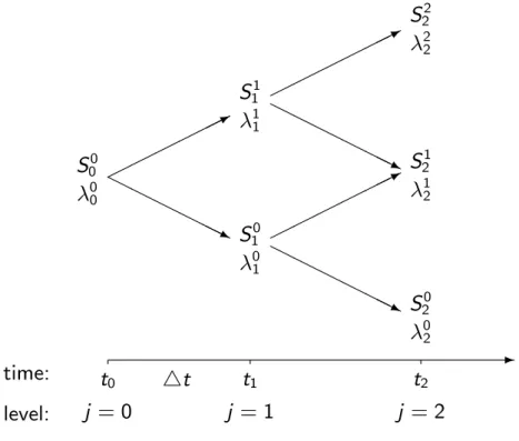
-t0 j = 0 t1 j = 1 t2 j = 2 4t time: level: * H H H H HHj * H H H H H_Hj * H H H H H_Hj S00 λ00 S11 λ11 S22 λ22 S10 λ01 λ02 S20 S21 λ12

Figure 10.1. Construction of an implied binomial tree.

Figure 10.1 illustrates the construction of the first two nodes of an IBT. We build the IBT on the time interval [0, T] with j = 0,1,2, . . . , n equally spaced

levels, 4tapart. We start at zero level with t = 0, here the stock price equals the current price of the underlying: S₀0 = S. There aren+ 1 nodes at the nth level of the tree, we indicate the stock price of the ith node at the nth level by S_ni, and the forward price at level n+ 1 of S_ni at level n by F_ni = er4tS_ni. The conditional probability pn_i+1 = P(Sn+1 = Sni+1+1|Sn = Sni) is the transition

probability of making a transition from node (n, i) to node (n+ 1, i+ 1). The forward price Fn,i is required to satisfy the risk neutral condition:

F_ni = pn_i+1S_ni+1₊₁ + (1−pn_i+1)S_ni₊₁ . (10.7)

Thus we obtain the transition probability from the following equation: pn_i+1 = F

i

n−Sni+1

S_ni+1₊₁−S_ni₊₁ . (10.8)

The Arrow-Debreu price is the price of an option which pays 1 unit payoff if the stock price St at time t attains the value Sni, and 0 otherwise. The

Arrow-Debreu price in the state i at level ncan be computed as the expected discounted value of its payoff: λi_n = E[e−rt1(St = Sni)|S0 = S00]. In general,

Arrow-Debreu prices can be obtained by the iterative formula, where λ0₀ = 1 as a definition.

λ0_n+1 = e−r4tλ0_n(1−pn₁)

λi_n+1₊₁ = e−r4tλi_npn_i+1 +λi_n+1(1−pn_i+2) , 0≤ i ≤ n−1 (10.9) λn_n+1₊₁ = e−r4t{λn_npn_n+1}

To illustrate the calculation of the Arrow-Debreu prices, we provide an ex-ample with a construction of a CRR binomial tree. Let us assume that the current value of the underlying S = 100, time to maturity τ = T = 2 years, 4t= 1 year, constant volatility σ = 10%, and riskless interest rate r = 0.03. The Arrow-Debreu price tree shown in the Figure 10.3 can be calculated from the stock price tree in the Figure 10.2.

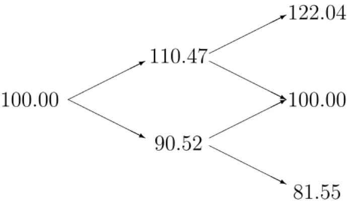
Using the CRR method, the stock price at the lower node at the first level equals S₁0 = S₀0 · e−σ4t = 100 · e−0.1 = 90.52, and at the upper node S₁1 = S₀0 · eσ4t = 110.47. The transition probability p0₁ = 0.61 is obtained by the formula (10.8) with F₀0 = S₀0e0.03 = 103.05. Now, we calculate λi₁ for i = 0,1, according to the formula (10.9): λ0₁ = e−r4t · λ0₀ · (1− p0₁) = 0.36 and λ1₁ = e−r4t · λ0₀ ·p0₁ = 0.61. At the second level, we calculate the stock prices according to the corresponding nodes at the first level, for example: S₂0 = S₁0 · e−σ4t = 81.55, S₂1 = S₀0 = 100 and S₂2 = S₁1 · eσ4t = 122.04.

* H H H H HHj * H H H H HHj * H H H H HHj 100.00 110.47 90.52 122.04 100.00 81.55

Figure 10.2. CRR binomial tree for stock prices with T = 2 years, 4t= 1, σ = 0.1 and r = 0.03. XFGIBT01

* H H H H HHj * H H H H HHj * H H H H HHj 1.00 0.61 0.36 0.37 0.44 0.13

Figure 10.3. CRR binomial tree for Arrow-Debreu prices with T = 2 years, 4t= 1, σ = 0.1 and r = 0.03. XFGIBT01

The corresponding Arrow-Debreu prices λi₂ for i = 0,1,2 are obtained by the substitution in the formula 10.9:

λ0₂ = e−r4t ·λ0₁ ·(1−p1₁) = 0.13

λ1₂ = e−r4t · {λ0₁ ·p1₁ +λ1₁ ·(1−p1₂) = 0.44} λ2₂ = e−r4t ·λ1₁ ·p1₂ = 0.37 .

prices are given by: C(K, τ) = e−rτ Z +∞ 0 max(ST −K,0)q(ST|St, r, τ)dST, (10.10) P(K, τ) = e−rτ Z +∞ 0 max(K −ST,0)q(ST|St, r, τ)dST , (10.11)

where C(K, τ) and P(K, τ) denote call option price and put option price respectively, andK is the strike price. In the IBT, option prices are calculated in discrete time intervals τ = n4t using the Arrow-Debreu prices,

C(K, n4t) = n X i=0 λi_n+1₊₁max(S_ni+1₊₁ −K,0) , (10.12) P(K, n4t) = n X i=0 λi_n+1₊₁max(K −S_ni+1₊₁,0) . (10.13)

Using the risk neutral condition (10.7) and the discrete option price calcula-tion from (10.12) or (10.13), one obtains the iteracalcula-tion formulae to construct the IBT.

Let us assume the strike price is equal to the known stock price: K = S_ni = S. Then the contribution from the transition to the first in-the-money upper node can be separated from the other contributions. Using the iterative formulae for the Arrow-Debreu prices (10.9) in the equation (10.12):

er4tC(S, n4t) = λ0_n(1−pn₁) max(S_n0₊₁ −S,0) +λn_np_nn₊₁max(S_nn₊₁+1 −S,0) + n−1 X j=0 n λ_njpn_j+1 +λ_nj+1(1−pn_j+2) o max(S_nj+1₊₁ −S,0) = λi_npn_i+1+ λ_ni+1(1−pn_i+2) (S_ni+1₊₁−S) +λn_np_nn₊₁(S_nn₊₁+1 −S) + n−1 X j=i+1 λj_npn_j+1 +λj_n+1 1−pn_j+2 (S_nj+1₊₁ −S) = λi_npn_i+1(S_ni+1₊₁−S) + n−1 X j=i+1 λj_npn_j+1(S_nj+1₊₁−S) +λn_npn_n+1(S_nn₊₁+1 −S) +λi_n+1(1−pn_i+2)(S_ni+1₊₁ −S) + n X j=i+2 λj_n(1−pn_j+1)(S_nj₊₁−S) = λi_npn_i+1(S_ni+1₊₁−S) + n X j=i+1 λj_n n 1−pn_j+1(S_nj₊₁ −S) +pn_j+1(S_nj+1₊₁ −S) o .

Entering the risk neutral condition (10.7) in the last term, one obtains: er4tC(S, n4t) =λi_npn_i+1 S_ni+1₊₁ −S+

n

X

j=i+1

λj_n F_nj −S . (10.14)

Now, the stock price for the upper node can be rewritten in terms of the known Arrow-Debreu prices λi_n, the known stock prices S_ni and the known forwards F_ni: S_ni+1₊₁ = S i n+1 C S_ni, n4ter4t −ρu −λinSni Fni −Sni+1 C(Si n, n4t)er4t −ρu−λin Fni −Sni+1 , (10.15)

where ρu denotes the following summation term:

ρu = n

X

j=i+1

λj_n(F_nj −S_ni) . (10.16)

The transition from the nth to the (n+ 1)th level of the tree is defined by (2n+ 3) parameters, i.e. (n+ 2) stock prices of the nodes at the (n+ 1)th

level, and (n+ 1) transition probabilities (when the IBT starts at the zero-level). Suppose (2n+1) parameters corresponding to thenth level are known, the stock prices S_ni₊₁ and transition probabilities pn_i+1 at all nodes above the centre of the tree corresponding to the (n+ 1)th level can be found iteratively using the equations (10.15) and (10.8) as follows:

We always start from the central nodes, if n is odd, define S_ni₊₁ = S₀0 = S, for i = (n + 1)/2. If n is even, we start from the two central nodes just below and above the centre of the level, S_ni₊₁ and S_ni+1₊₁ for i = n/2, and set S_ni₊₁ = (S_ni)2/S_ni+1₊₁ = S2/S_ni+1₊₁, which adjusts the logarithmic CRR centring spacing between S_ni and S_ni+1₊₁ to be the same as that between S_ni and S_ni₊₁. Substituting this relation into (10.15) one gets the formula for the upper of the two central nodes for the odd levels:

S_ni+1₊₁ = S C(S, n4t)er4t +λi_nS −ρu λi nFni −er4tC(S, n4t) + ρu for i = n 2 . (10.17)

Once we have the initial nodes’ stock prices, according to the relationships among the different parameters, we can repeat the process to calculate those at higher nodes (n+ 1, j), j = i+ 2, . . . n+ 1 one by one.

Similarly, we can calculate the parameters at lower nodes (n + 1, j), j = i−1, . . . ,1 at the (n+ 1)th level by using the known put prices P(K, n4t) for K = S_ni. S_ni₊₁ = S i+1 n+1 er4tP(S_ni, n4t)−ρl −λinSni(Fni −S i+1 n+1) er4t_{P {S}i n,(n+ 1)4t} −ρl +λin(Fni −S i+1 n+1) , (10.18)

where ρl denotes the sum over all nodes below the one with price Sni:

ρl = i−1

X

j=0

λj_n(S_ni −F_nj) . (10.19)

Transition probabilities and Arrow-Debreu prices are obtained by (10.8) and (10.9), respectively.

C(K, τ) and P(K, τ) in (10.15) and (10.18) are the interpolated values for a call or put struck today at strike price K and time to maturity τ. In the DK construction, they are obtained by the CRR binomial tree with constant parameters σ = σimp(K, τ), calculated from the known market option prices.

In practice, calculating interpolated option prices by the CRR method is computationally intensive.

10.1.2 Compensation

The transition probability pn_i at any node should lie between 0 and 1, this condition avoids the riskless arbitrage: ifpn_i+1 > 1, the stock priceS_ni+1₊₁ would fall below the forward price F_ni, similarly, if pn_i+1 < 0, the strike price S_ni₊₁ would fall above the forward price F_ni. Therefore it is useful to limit the estimated stock prices by the neighbouring forwards from the previous level: F_ni < S_ni+1₊₁ < F_ni+1 . (10.20) If the stock price does not fulfil the above inequality condition, we rede-fine it by assuming that the logaritmic difference between the stock prices at this node and its adjacent is equal to the logaritmic difference between the corresponding stock prices at the two nodes at the previous level, i.e., log(S_ni+1₊₁/S_ni₊₁) = log(S_ni/S_ni−1). Sometimes, the obtained price still does not satisfy inequality (10.20), then we substitute the stock price S_ni+1₊₁ by the average of F_ni and F_ni+1.

As used in the construction of the IBT in (10.12) or (10.13), the implied conditional distribution, the SPDq(ST|St, r, τ), could be estimated at discrete

timeτ = n4tby the product of the Arrow-Debreu pricesλi_n+1 at the (n+1)th level with the influence of the interest rate ern4t. To fulfill the risk-neutrality condition (10.7), the conditional expected value of the underlying log stock price in the following (n+ 1)th level, given the stock price at the nth level is defined as: M = EQ{log(Sn+1)|Sn = Sni} = p n i+1log(S i+1 n+1)+(1−p n i+1) log(S i n+1) . (10.21)

We can specify such a condition also for the conditional second moments of log(Sn+1) at Sn = Sni, which is the implied local volatility σ2(Sni, n4t) during

the time period 4t:

σ2(S_ni,4t) = VarQ{log(Sn+1)|Sn = Sni} = pn_i+1{log(S_ni+1₊₁)−M}2 + (1−pn_i+1){log(S_ni₊₁)−M}2 = 2 log S_ni+1₊₁ S_ni₊₁ {pn_i+1(1−pn_i+1)} . (10.22)

After the construction of an IBT, all stock prices, transition probabilities, and Arrow-Debreu prices at any node in the tree are known. We are thus able to calculate the local volatility σ(S_ni, m4t) at any level m.

In general, the instantaneous volatility function used in the diffusion model (10.6) is different from the local volatility function derived in (10.22), only in the BS model are they identical. Additional, the BS implied volatility

b

σ(K, τ), which assumes the Black-Scholes model at least locally, differs from the local volatilityσ(s, τ), they describe different characteristics of the second moment using different parameters.

If we choose 4t small enough, we obtain the estimated SPD at fixed time to maturity, and the distribution of local volatility σ(S, τ).

10.1.3 Barle and Cakici Algorithm

Barle and Cakici (1998) (BC) suggest an improvement of the DK construc-tion. The first major modification is the choice of the strike price in which the option should be evaluated (as in 10.14). In the BC algorithm, the strike price K is chosen to be equal to the forward price F_ni, and similarly to the DK construction, using the discrete approximation (10.12) we get:

er4tC(F_ni, n4t) = n X j=0 λ_nj+1₊₁max(S_nj+1₊₁ −F_ni,0) = λi_npn_i+1 +λ_ni+1(1−pn_i+2) (S_ni+1₊₁−F_ni) +λn_np_nn₊₁(S_nn₊₁+1 −F_ni) + n−1 X j=i+1 λj_npn_j+1 +λj_n+1 1−pn_j+2 (S_nj+1₊₁ −F_ni) = λi_npn_i+1(S_ni+1₊₁ −F_ni) + n X j=i+1 λj_n n 1−pn_j+1(S_nj₊₁−F_ni) +pn_j+1(S_nj+1₊₁−F_ni) o .

Entering the risk neutral condition again (10.7) one obtains: er4tC(F_ni, n4t) = λ_nipn_i+1 S_ni+1₊₁−F_ni+

n

X

j=i+1

λj_n F_nj −F_ni . (10.23)

Identify the upper sum as: %u =

n

X

j=i+1

λj_n F_nj −F_ni , (10.24)

and using the equation for the transition probability (10.8) we can write the recursion relation for the stock price in the upper node as follows:

S_ni+1₊₁ = S i n+1 C F_ni, n4ter4t −%u −λinFni Fni −Sni+1 C (Fi n, n4t)er4t −%u−λin Fni −Sni+1 . (10.25)

Analogous to the DK construction, we start from the central nodes of the binomial tree, but in contrast with the DK construction the BC construction takes the riskless interest rate into account. If (n+ 1) is even, the price of the central node S_ni₊₁ = S₀0er4t for i = (n+ 1)/2. If (n+ 1) is odd, the two central nodes must satisfy S_ni₊₁·S_ni+1₊₁ = (F_ni)2. Adding this condition to the equation (10.25) the lower central node can be calculated as:

S_ni₊₁ = F_niλ i nF i n− {e r4t_C(Fi n, n4t)−%u} λi nFni + {er4tC(Fni, n4t)−%u} for i = 1 +n/2, (10.26) the upper one is then: S_ni+1₊₁ = (F_ni)2/S_ni₊₁.

After stock prices of the central nodes are obtained, we repeat the recursion equation (10.25) to calculate the stock prices at higher nodes (n+ 1, j), j = i + 2, . . . , n+ 1. The transition probabilities and Arrow-Debreu prices are calculated through (10.8) and (10.9), respectively.

Similarly, an analogous recursion relation for the stock prices at lower nodes can be found by using put option prices at strike F_ni:

S_ni₊₁ = S i+1 n+1{P(F i n, n4t)er4t −%l}λinFni(S i+1 n+1−F i n) P(Fi n, n4t)er4t −%l −λin(S i+1 n+1−Fni) , (10.27)

where where %l denotes the lower sum:

%l = i−1

X

j=0

λj_n(F_ni −F_nj) .

Notice that BC use the Black-Scholes call and put option prices C(K, τ) and P(K, τ), which makes the calculation faster than the interpolation technique based on the CRR method.

The balancing inequality (10.20), to avoid negative transition probabilities, and therewith the arbitrage is still used in the BC algorithm: they re-estimate S_ni+1₊₁ by the average of F_ni and F_ni+1, though the choice of any point between these forward prices is sufficient.

10.2 A Simulation and a Comparison of the

SPDs

The following detailed example illustrates the construction of the tree from the smile, using the DK algorithm first, and the BC algorithm afterwards.

Let us assume that the current value of the underlying stock S = 100, with no dividend and the annually compounded riskless interest rate r = 3% per year for all time expirations. For the implied volatility function, we use a convex function:

b

σ = −0.2

{log(K/St)}2 + 1

+ 0.3, (10.28)

taken from Fengler (2005). For simplicity, we do not model a term structure of the implied volatility. The BS option prices needed for growing the tree are calculated from this implied volatility function. We construct the IBTs with time to maturity T = 1 year discretized in five time steps.

10.2.1 Simulation Using the DK Algorithm

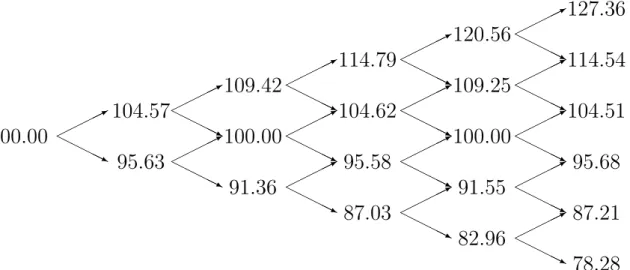
Using the assumption on the BS implied volatility surface described above, we obtain the one year stock price implied binomial tree (Figure 10.4), the upward transition probability tree (Figure 10.5), and the Arrow-Debreu price tree (Figure 10.6). * H H H_Hj * H H H_Hj * H H H_Hj * H H H_Hj * H H H_Hj * H H H_Hj * H H H_Hj * H H H_Hj * H H H_Hj * H H H_Hj * H H H_Hj * H H H_Hj * H H H_Hj * H H H_Hj * H H H_Hj 100.00 104.57 95.63 109.42 100.00 91.36 114.79 104.62 95.58 87.03 120.56 109.25 100.00 91.55 82.96 127.36 114.54 104.51 95.68 87.21 78.28 Figure 10.4. Stock price tree calculated with the DK al-gorithm with S₀0 = 100, r = 0.03 and T = 1 year.

XFGIBT01

All the IBTs correspond to time to maturity τ = 1 year, and 4t= 1/5 year. Figure 10.4 shows the estimated stock prices starting at the zero level with S₀0 = S = 100. The elements in the j-th column correspond to the (j −1)th level of the stock price tree. Figure 10.5 shows the transition probabilities, its element (n, j) represents the transition probability from the node (n−1, j−1) to the node (n, j). The third tree displayed in Figure 10.6 contains the Arrow-Debreu prices. Its elements in the j-th column match the Arrow-Debreu

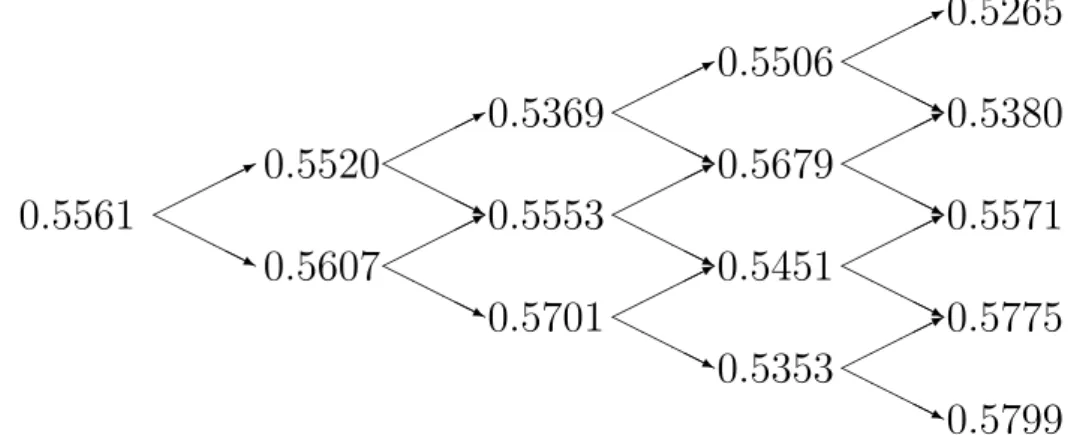
* H H H_Hj * H H H_Hj * H H H_Hj * H H H_Hj * H H H_Hj * H H H_Hj * H H H_Hj * H H H_Hj * H H H_Hj * H H H_Hj 0.5561 0.5520 0.5607 0.5369 0.5553 0.5701 0.5506 0.5679 0.5451 0.5353 0.5265 0.5380 0.5571 0.5775 0.5799

Figure 10.5. Transition probability tree calculated with the

DK algorithm with S₀0 = 100, r = 0.03 and T = 1

year. XFGIBT01 * H H H_Hj * H H H_Hj * H H H_Hj * H H H_Hj * H H H_Hj * H H H_Hj * H H H_Hj * H H H_Hj * H H H_Hj * H H H_Hj * H H H_Hj * H H H_Hj * H H H_Hj * H H H_Hj * H H H_Hj 1.0000 0.5528 0.4412 0.3033 0.4921 0.1927 0.1619 0.4112 0.3267 0.0823 0.0886 0.3045 0.3536 0.1916 0.0380 0.0464 0.2045 0.3357 0.2656 0.1024 0.0159

Figure 10.6. Arrow-Debreu price tree calculated with the DK algorithm with S₀0 = 100, r = 0.03 and T = 1 year.

XFGIBT01

prices in the (j − 1) th level. Using the stock prices together with Arrow-Debreu prices of the nodes at the final level, a discrete approximation of the implied price distribution can be obtained. Notice that by the definition of the Arrow-Debreu price, the risk neutral probability corresponding to each node should be calculated as the product of the Arrow-Debreu price and the factor erj4t in the level j.

Choosing the time steps small enough, we obtain more accurate estimation of the implied price distribution and the local volatility surface σ(S, τ). We

still use the same implied volatility function from (10.28), and assume S₀0 = 100, r = 0.03 , T = 5 years.

SPD estimation arising from fitting the implied five-year tree with 40 levels is shown in Figure 10.7. Local volatility surface computed from the implied tree at different times to maturity and stock price levels is shown in Figure 10.8. Obviously, the local volatility captures the volatility smile, which decreases with the strike price and increases with the time to maturity.

60 80 100 120 140 160 180 200

0 0.005 0.01 0.015

Estimated Implied Distribution

Stock Price

Probability

Figure 10.7. SPD estimation by the DK IBT computed with S₀0 = 100, r = 0.03 and T = 5 years. XFGIBT02

10.2.2 Simulation Using the BC Algorithm

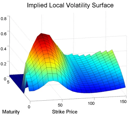
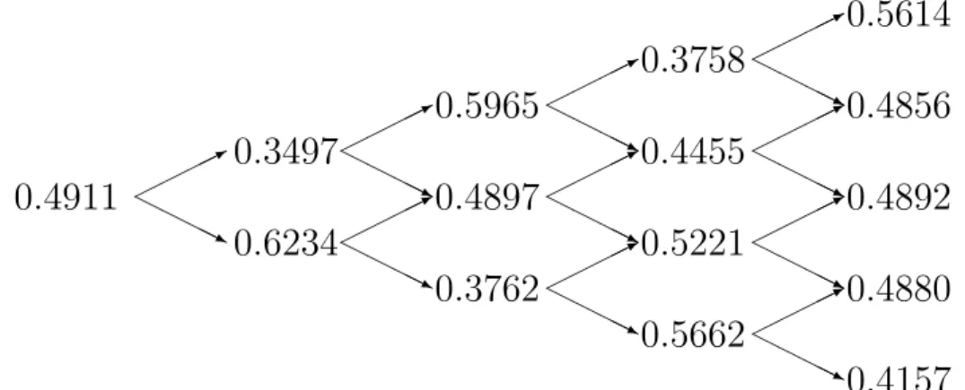
The BC algorithm can be applied in analogy to the DK technique. The computing part is replaced by the BC algorithm, we are using the implied volatility function from (10.28) as in the DK algorithm. Figures 10.9 - 10.11 show the one-year stock price tree with five steps, transition probability tree, and Arrow-Debreu tree. Figure 10.12 presents the plot of the estimated SPD by fitting a five year implied binomial tree with 40 levels using BC algorithm. Figure 10.13 shows the characteristics of the local volatility surface of the generated IBT, the local volatility follows the “volatility smile”, which decreases with the stock price and increases with time.

Figure 10.8. Implied local volatility surface estimated by the DK IBT with S₀0 = 100, r = 0.03 and T = 5 years.

XFGIBT02 . * H H H_Hj * H H H_Hj * H H H_Hj * H H H_Hj * H H H_Hj * H H H_Hj * H H H_Hj * H H H_Hj * H H H_Hj * H H H_Hj * H H H_Hj * H H H_Hj * H H H_Hj * H H H_Hj * H H H_Hj 100.00 104.26 97.08 111.72 101.21 91.79 116.66 106.09 97.72 89.09 126.15 112.07 102.43 93.80 84.18 133.71 118.20 107.59 98.69 90.25 80.73

Figure 10.9. Stock price tree calculated with the BC algorithm with S₀0 = 100, r = 0.03 and T = 1 year. XFGIBT01

10.2.3 Comparison with the Monte-Carlo Simulation

We now compare the SPD estimation obtained by the two IBT methods with the estimated density function of a simulated process St generated from

* H H H_Hj * H H H_Hj * H H H_Hj * H H H_Hj * H H H_Hj * H H H_Hj * H H H_Hj * H H H_Hj * H H H_Hj * H H H_Hj 0.4911 0.3497 0.6234 0.5965 0.4897 0.3762 0.3758 0.4455 0.5221 0.5662 0.5614 0.4856 0.4892 0.4880 0.4157

Figure 10.10. Transition probability tree calculated with the BC algorithm with S₀0 = 100, r = 0.03 and T = 1 year.

XFGIBT01 * H H H_Hj * H H H_Hj * H H H_Hj * H H H_Hj * H H H_Hj * H H H_Hj * H H H_Hj * H H H_Hj * H H H_Hj * H H H_Hj * H H H_Hj * H H H_Hj * H H H_Hj * H H H_Hj * H H H_Hj 1.0000 0.4881 0.5059 0.1697 0.6290 0.1894 0.1006 0.3743 0.3889 0.1174 0.0376 0.2282 0.4086 0.2513 0.0506 0.0210 0.1265 0.3154 0.3294 0.1488 0.0294

Figure 10.11. Arrow-Debreu price tree calculated with the BC algorithm with S₀0 = 100, r = 0.03 and T = 1 year.

XFGIBT01

the diffusion process (10.6). To perform a discrete approximation of this diffusion process, we use the Euler scheme with time step δ = 1/1000, the constant drift µt = r = 0.03 and the volatility function σ(St, t) =

−0.2 {log(K/St)}2 + 1 + 0.3 .

Compared to Sections 10.2.2 and 10.2.2 where we started from the BS implied volatility surface, here we construct the IBTs direct from the simulated option price function. In the construction of the IBTs, we calculate the option prices

50 100 150 200 0

0.005 0.01 0.015

Estimated Implied Distribution

Stock Price

Probability

Figure 10.12. SPD estimation by the BC IBT computed with S₀0 = 100, r = 0.03 and T = 5 years. XFGIBT02

Figure 10.13. Implied local volatility surface estimated by the BC IBT withS₀0 = 100,r = 0.03 andT = 5 years. XFGIBT02

corresponding to each node at the implied tree according to their theoretical definitions (10.3) and (10.3) from the simulated asset prices St. We simulate

Monte-Carlo simulation method. 80 90 100 110 120 130 140 150 160 0 0.01 0.02 0.03 0.04 0.05 0.06

Estimated State Price Density

Stock Price

Probability

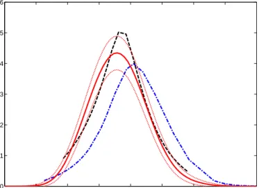
Figure 10.14. SPD estimation from the DK IBT (blue dashed line) and from the BC IBT (black dashed line) compared to the estimation by Monte-Carlo simulation with its 95% con-fidence band (red lines). Level = 50, T = 5 years, 4t = 0.1

year. XFGIBT03

From the estimated distribution shown in Figure 10.14, we observe small deviations of the SPDs obtained from the two IBT methods from the esti-mation obtained by the Monte-Carlo simulation. The SPD estiesti-mation by the BC algorithm coincides substantially better with the estimation from the simulated process than the estimation by the DK algorithm, which shows a shifted mean of its SPD.

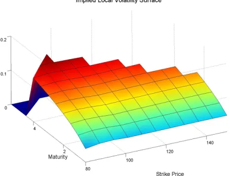
As above, we can also estimate the local volatility surface from the both im-plied binomial trees. Compare Figure 10.15 with Figure 10.16 and notice that some edge values cannot be obtained directly from the five-year IBT. How-ever, both local volatility surface plots actually coincide with the volatility smile characteristic, the implied local volatility of the out-the-money options decreases with the increasing stock price, and increases with time.

10.3 Example – Analysis of EUREX Data

In the following example we use the IBTs to estimate the price distribution of the real stock market data. We use underlying asset prices, strike prices, time to maturity, interest rates, and call/put option prices from EUREX at 19

Figure 10.15. Implied local volatility surface of the simulated model, calculated from DK IBT. XFGIBTcdk

Figure 10.16. Implied local volatility surface of the simulated model, calculated from BC IBT. XFGIBTcbc

March, 2007, taken from the database of German stock exchange. First, we estimate the BS implied volatility surface from the data set with the technique

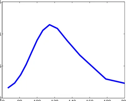
Figure 10.17. BS implied volatility surface estimated from real stock and option prices. XFGIBT05

of Fengler, H¨ardle and Villa (2003). Figure 10.17 shows the estimated implied volatility surface, which reflects the characteristics that the implied volatility decreases with the strike price and increases with time to maturity.

Now we construct the IBTs, where we calculate the interpolated option prices with the CRR binomial tree method using the estimated implied volatility. Fitting the function of option prices directly from the market option prices causes difficulties since the function approaches a value of zero for very high strike prices which would violate no-arbitrage conditions.

The estimated stock price distribution, obtained by the BC and the DK IBT with 40 levels, forτ = 0.5 year, is shown in Figure 10.18. Obviously, the both estimated SPDs are nearly identical. The SPDs do not show any deviations from the log-normal characteristics according to their skewness and kurtosis.

From the simulations and real data example, we conclude that the implied binomial tree is a simple smile-consistent method to assess the future stock prices. Still, some limitations of the algorithms remain. With an increasing interest rate or with a small time step, negative transition probabilities occur more often. When the interest rate is high, the BC algorithm is a better choice. The DK algorithm cannot handle with higher interest rates such as r = 0.2, in this case the BC algorithm still can be used. In addition, the negative probabilities appear more rarely in the BC algorithm than in

50000 5200 5400 5600 5800 6000 6200 0.5 1 1.5 2 2.5 3x 10

-3 Estimated State Price Density

Stock Price

Probability

Figure 10.18. SPD estimation by the BC IBT (black dashed line) and by the DK IBT (blue solid line) from the EUREX data, τ = 0.5 year, level = 25. XFGIBT05

the DK construction, even though most of them appear at the edge of the trees. But, by modifying these values we are effectively losing the information about the volatility behavior at the corresponding nodes. This deficiency is a consequence of our condition that continuous diffusion process is modeled as a discrete binomial process. Improving of this requirement leads to a transition to multinomial or varinomial trees which have a drawback of more complicated models with difficult realization.

Besides its basic function to price derivatives in consistency with market prices, IBTs are also useful for hedging, calculating local volatility surfaces or estimation of the future price distribution according to the historical data. In the practical application, the reliability of the approach depends critically on the quality of the dynamics estimation of the underlying process, such as of the BS implied volatility surface obtained from the market option prices.

Bibliography

Ait-Sahalia, Y. and Lo, A. (1998). Nonparametric Estimation of State-Price Densities

Im-plicit in Financial Asset Prices, Journal of Finance, 53: 499–547.

Ait-Sahalia, Y. , Wang, Y. and Yared, F.(2001). Do Option Markets Correctly Price the

110.

Barle, S. and Cakici, N. (1998). How to Grow a Smiling Tree The Journal of Financial

Engineering,7: 127–146.

Bingham, N.H. and Kiesel, R. (1998). Risk-neutral Valuation: Pricing and Hedging of

Financial Derivatives, Springer Verlag, London.

Cox, J., Ross, S. and Rubinstein, M. (1979). Option Pricing: A simplified Approach,Jouranl

of Financial Economics 7: 229–263.

Derman, E. and Kani, I. (1994). The Volatility Smile and Its Implied Tree

http://www.gs.com/qs/

Derman, E. and Kani, I. (1998). Stochastic Implied Trees: Arbitrage Pricing with Stochastic

Term and Strike Structure of Volatility,International Journal of Theroetical and Applied

Finance1: 61–110.

Dupire, B. (1994). Pricing with a Smile, Risk7: 18–20.

Fengler, M. R.(2005). Semiparametric Modeling of Implied Volatility, Springer Verlag,

Hei-delberg.

Fengler, M. R., H¨ardle, W. and Villa, Chr. (2003). The Dynamics of Implied Volatilities: A

Common Principal Components Approach,Review of Derivative Research 6: 179–202.

H¨ardle, W., Hl´avka, Z. and Klinke, S. (2000). XploRe Application Guide, Springer Verlag,

Heidelberg.

Hui, E.C. (2006). An enhanced implied tree model for option pricing: A study on Hong Kong

property stock options,International Review of Economics and Finance 15: 324–345.

Hull, J. and White, A. (1987). The Pricing of Options on Assets with Stochastic Volatility, Journal of Finance42: 281–300.

Jackwerth, J. (1999). Optional-Implied Risk-Neutral Distributions and Implied Binomial

Trees: A Literature Review,Journal of Finance 51: 1611–1631.

Jackwerth, J. and Rubinstein, M. (1996). Recovering Probability Distributions from Option

Prices, Journal of Finance51: 1611–1631.

Kim, I.J. and Park, G.Y. (2006). An empirical comparison of implied tree models for KOSPI

200 index options, International Review of Economics and Finance 15: 52–71.

Kloeden, P., Platen, E. and Schurz, H. (1994).Numerical Solution of SDE Through Computer

Experiments, Springer Verlag, Heidelberg.

Merton, R. (1976). Option Pricing When Underlying Stock Returns are Discontinuous, Journal of Financial EconomicsJanuary-March: 125–144.

Moriggia, V., Muzzioli,S. and Torricelli, C. (2007). On the no-arbitrage condition in option

implied trees,European Journal of Operational Research forthcoming.

Muzzioli,S. and Torricelli, C. (2005). The pricing of options on an interval binomial tree. An

application to the DAX-index option market,European Journal of Operational Research

163: 192–200.

Rubinstein, M. (1994). Implied Binomial Trees. Journal of Finance 49: 771–818.

Yatchew, A. and H¨ardle,W. (2006). Nonparametric state price density estimation using

For a complete list of Discussion Papers published by the SFB 649, please visit http://sfb649.wiwi.hu-berlin.de.

001 "Testing Monotonicity of Pricing Kernels" by Yuri Golubev, Wolfgang Härdle and Roman Timonfeev, January 2008.

002 "Adaptive pointwise estimation in time-inhomogeneous time-series models" by Pavel Cizek, Wolfgang Härdle and Vladimir Spokoiny, January 2008.

003 "The Bayesian Additive Classification Tree Applied to Credit Risk Modelling" by Junni L. Zhang and Wolfgang Härdle, January 2008.

004 "Independent Component Analysis Via Copula Techniques" by Ray-Bing Chen, Meihui Guo, Wolfgang Härdle and Shih-Feng Huang, January 2008.

005 "The Default Risk of Firms Examined with Smooth Support Vector Machines" by Wolfgang Härdle, Yuh-Jye Lee, Dorothea Schäfer and Yi-Ren Yeh, January 2008.

006 "Value-at-Risk and Expected Shortfall when there is long range dependence" by Wolfgang Härdle and Julius Mungo, Januray 2008. 007 "A Consistent Nonparametric Test for Causality in Quantile" by

Kiho Jeong and Wolfgang Härdle, January 2008.

008 "Do Legal Standards Affect Ethical Concerns of Consumers?" by Dirk Engelmann and Dorothea Kübler, January 2008.

009 "Recursive Portfolio Selection with Decision Trees" by Anton Andriyashin, Wolfgang Härdle and Roman Timofeev, January 2008.

010 "Do Public Banks have a Competitive Advantage?" by Astrid Matthey, January 2008.

011 "Don’t aim too high: the potential costs of high aspirations" by Astrid Matthey and Nadja Dwenger, January 2008.

012 "Visualizing exploratory factor analysis models" by Sigbert Klinke and Cornelia Wagner, January 2008.

013 "House Prices and Replacement Cost: A Micro-Level Analysis" by Rainer Schulz and Axel Werwatz, January 2008.

014 "Support Vector Regression Based GARCH Model with Application to Forecasting Volatility of Financial Returns" by Shiyi Chen, Kiho Jeong and Wolfgang Härdle, January 2008.

015 "Structural Constant Conditional Correlation" by Enzo Weber, January 2008.

016 "Estimating Investment Equations in Imperfect Capital Markets" by Silke Hüttel, Oliver Mußhoff, Martin Odening and Nataliya Zinych, January 2008.

017 "Adaptive Forecasting of the EURIBOR Swap Term Structure" by Oliver Blaskowitz and Helmut Herwatz, January 2008.

018 "Solving, Estimating and Selecting Nonlinear Dynamic Models without the Curse of Dimensionality" by Viktor Winschel and Markus Krätzig, February 2008.

019 "The Accuracy of Long-term Real Estate Valuations" by Rainer Schulz, Markus Staiber, Martin Wersing and Axel Werwatz, February 2008. 020 "The Impact of International Outsourcing on Labour Market Dynamics in

Germany" by Ronald Bachmann and Sebastian Braun, February 2008. 021 "Preferences for Collective versus Individualised Wage Setting" by Tito

Boeri and Michael C. Burda, February 2008.

SFB 649, Spandauer Straße 1, D-10178 Berlin http://sfb649.wiwi.hu-berlin.de

This research was supported by the Deutsche

SFB 649, Spandauer Straße 1, D-10178 Berlin http://sfb649.wiwi.hu-berlin.de

This research was supported by the Deutsche

Forschungsgemeinschaft through the SFB 649 "Economic Risk". S&P 500 Firms" by Jörn Hendrich Block, February 2008.

024 "Skill Specific Unemployment with Imperfect Substitution of Skills" by Runli Xie, March 2008.

025 "Price Adjustment to News with Uncertain Precision" by Nikolaus Hautsch, Dieter Hess and Christoph Müller, March 2008.

026 "Information and Beliefs in a Repeated Normal-form Game" by Dietmar Fehr, Dorothea Kübler and David Danz, March 2008.

027 "The Stochastic Fluctuation of the Quantile Regression Curve" by Wolfgang Härdle and Song Song, March 2008.

028 "Are stewardship and valuation usefulness compatible or alternative objectives of financial accounting?" by Joachim Gassen, March 2008. 029 "Genetic Codes of Mergers, Post Merger Technology Evolution and Why

Mergers Fail" by Alexander Cuntz, April 2008.

030 "Using R, LaTeX and Wiki for an Arabic e-learning platform" by Taleb Ahmad, Wolfgang Härdle, Sigbert Klinke and Shafeeqah Al Awadhi, April 2008.

031 "Beyond the business cycle – factors driving aggregate mortality rates" by Katja Hanewald, April 2008.

032 "Against All Odds? National Sentiment and Wagering on European Football" by Sebastian Braun and Michael Kvasnicka, April 2008.

033 "Are CEOs in Family Firms Paid Like Bureaucrats? Evidence from Bayesian and Frequentist Analyses" by Jörn Hendrich Block, April 2008. 034 "JBendge: An Object-Oriented System for Solving, Estimating and

Selecting Nonlinear Dynamic Models" by Viktor Winschel and Markus Krätzig, April 2008.

035 "Stock Picking via Nonsymmetrically Pruned Binary Decision Trees" by Anton Andriyashin, May 2008.

036 "Expected Inflation, Expected Stock Returns, and Money Illusion: What can we learn from Survey Expectations?" by Maik Schmeling and Andreas Schrimpf, May 2008.

037 "The Impact of Individual Investment Behavior for Retirement Welfare: Evidence from the United States and Germany" by Thomas Post, Helmut Gründl, Joan T. Schmit and Anja Zimmer, May 2008.

038 "Dynamic Semiparametric Factor Models in Risk Neutral Density Estimation" by Enzo Giacomini, Wolfgang Härdle and Volker Krätschmer, May 2008.

039 "Can Education Save Europe From High Unemployment?" by Nicole Walter and Runli Xie, June 2008.

042 "Gruppenvergleiche bei hypothetischen Konstrukten – Die Prüfung der Übereinstimmung von Messmodellen mit der Strukturgleichungs-methodik" by Dirk Temme and Lutz Hildebrandt, June 2008.

043 "Modeling Dependencies in Finance using Copulae" by Wolfgang Härdle, Ostap Okhrin and Yarema Okhrin, June 2008.

044 "Numerics of Implied Binomial Trees" by Wolfgang Härdle and Alena Mysickova, June 2008.