Department of Applied Mathematics Faculty of EEMCS University of Twente The Netherlands P.O. Box 217 7500 AE Enschede The Netherlands Phone: +31-53-4893400 Fax: +31-53-4893114 Email: [email protected] www.math.utwente.nl/publications Memorandum No. 1689
Detecting positive quadrant dependence and positive function dependence
A. Janic-Wr´oblewska,1 W.C.M. Kallenberg and T. Ledwina2
September, 2003
ISSN 0169-2690
1Institute of Mathematics, Wroclaw University of technology, Wybrze˙ze Wyspia´nskiego 27, 50-370 Wroclaw,
Poland
Detecting positive quadrant dependence
and positive function dependence
A. Janic-Wróblewska, W.C.M. Kallenberg and T. Ledwina
Institute of Mathematics
Wroc
ł
aw University of Technology
Wybrze
ze Wyspia´
˙
nskiego 27
50-370 Wroc
ł
aw
Poland
Faculty of Electrical Engineering, Mathematics and Computer Science
University of Twente
P.O. Box 217
7500 AE Enschede
The Netherlands
Institute of Mathematics
Polish Academy of Science
ul. Kopernika 18
51-617 Wroc
ł
aw
Abstract There is a lot of interest in positive dependence going beyond linear correlation. In this paper three new rank tests for testing independence against positive dependence are in-troduced. The first one is directed on positive quadrant dependence, the second and third one concentrate on positive function dependence. The new testing procedures are not only sensitive for positive grade linear correlation, but also for positive grade correlations of higher order. They are based on the principle of data driven tests, which consists of three steps. Firstly, parametric families are introduced spanning up the space of null hypothesis and alternatives; secondly, within the families good tests are used; thirdly, a selection rule determines the appro-priate model. The new tests improve standard tests for linear correlation as Spearman’s rank correlation test substantially in case some proper higher order correlations are exhibited by the data, while the loss in power under alternatives with dominating linear correlation is not very high. Monte Carlo results clearly show this behavior.
Keyword and phrases: positive quadrant dependence, positive function dependence, rank test, model selection, Monte Carlo study, projected Legendre polynomials.
2000 Mathematics Subject Classification: 62 G 10, 62 H 20, 65 C 05.
1
Introduction
Recently there is much attention on the effects of positive dependence among risks. Positive dependence may lead to substantial deviations, for instance in the stop-loss premiums, compared to the independence case; see e.g. Albers (1999), Denuit et al. (2001) and references therein. Another area, where positive (or negative) dependence is important is mathematical finance. For instance, one wish to know whether certain stocks are negatively dependent in order to build a well balanced portfolio. Also in many other fields there is a lot of interest in positive (or negative) dependence. The following citation from Mari and Kotz (2001) makes this clear. ”Examples of interdependent meteorological phenomena in nature and interdependence in the medical, social, and political aspects of our existence, not to mention the economic structures, are too numerous to be cited individually.”
The interest in positive dependence is not restricted to linear correlation. On the contrary, there is a still growing interest in going beyond linear correlation, see e.g. Embrechts et al. (2002). In this paper we concentrate on positive dependence, not restricting ourselves to linear correlation. Similar results can be formulated and proved for negative dependence, but see Remark 1.2.
The idea behind positive dependence of two random variablesX andY is the property that large (respectively small) values of X (or functions of X) go together with large (respectively small) values ofY (or functions ofY). This can be expressed in various ways resulting in many notions of positive dependence. Metry and Sampson (1991) introduce a family of 64 partial orders for positive dependence on bivariate distributions with fixed marginals. The fact that there are so many notions of "positive dependence" confirms the importance of and the high interest in the concept. For a review see e.g. Shaked (1979), Scarsini and Shaked (1996) or Joe (1997).
In view of the tremendous consequences of wrongly ignoring positive dependence in favour of independence, it is of great importance to test independence against the restricted alternative of positive dependence. Under bivariate normality dependence is completely described by linear correlation and therefore testing independence under bivariate normality is equivalent to testing linear correlation betweenX and Y. In general however,X and Y are independent if and only ifcov(f1(X), f2(Y)) = 0 for allf1 and f2 ranging over a separating class of functions (see e.g. Breiman (1968) page 165ff). Hence, linear correlation is, although being an important aspect of dependence, not the only one, as was already clear from the fact that there are so many notions of positive dependence.
In this paper we concentrate on testing independence against two types of positive depen-dence, called positive quadrant dependence (P QD) and positive function dependence (P F D). In fact, we like to develop tests which have high power at (strictly)P QD- andP F D-alternatives, respectively and low power at distributions which are not strictlyP QD and not strictly P F D, respectively. We look for tests which arrange their rejection region as much as possible on detect-ing distributions with positive dependence and have "low power" at distributions with negative dependence (or at distributions which are neither positive nor negative dependent). Although we are not formally testing "not positive dependent" (in the sense of P QD or P F D) against strictly positive dependent, from our point of view tests having high power at distributions which are not positive dependent give the wrong signal in such a problem.
New tests are introduced, which start with investigating linear correlation and consider step by step the correlation of larger and larger classes of functions. Since the marginal distributions of X and Y are unknown, we take the grade representation of the joint distribution of X and Y, that is we deal withF(X)andG(Y), whereF andGare the unknown marginal distribution functions of X and Y, respectively. The nonnegative (linear) correlation between F(X) and
G(Y) and the two types of positive dependence, P QD and P F D, can be described as follows: (tacitly it assumed that we restrict to existing covariances)
1. cov(F(X), G(Y))≥0 , that concerns linear correlation;
2. cov(f1(F(X)), f2(G(Y)))≥0for all nondecreasingf1andf2; this is equivalent withP QD (see Theorem 4.4 in Esary et al. (1967)); we speak of strictlyP QDwhen inequality holds for at least some pair of nondecreasing (f1,f2);
3. cov(f(F(X)), f(G(Y)))≥0 for allf; this isP F D (Joe (1997), page 25), or, equivalently, positive definite dependence, see Proposition 2.2 in Shaked (1979); we speak of strictly P F D when inequality holds for at least some functionf.
Remark 1.1 For all three forms the covariances are 0 in case of independence. Another still stronger notion of positive dependence is defined bycov(f1(F(X), G(Y)), f2(F(X), G(Y)))≥0 for allf1 and f2 nondecreasing in both arguments. The random variables X and Y are called associated when this holds (Esary et al. (1967)). However, taking f1(u, v) = f2(u, v) it is seen that independence ofX andY does not implycov(f1(F(X), G(Y)), f2(F(X), G(Y))) = 0, although independence of X and Y implies that X and Y are associated, see Theorem 2.1 in Esary et al. (1967). Therefore, we do not use this notion of positive dependence.
Remark 1.2 The concept of P F D deals with positive dependence of functions of X and Y. Its counterpart, negative function dependence, could be defined ascov(f(F(X)), f(G(Y)))≤0 for all f. Consider random variables X, Y both with as marginal distribution the uniform distribution on (0,1). When Y = 1−X one might intuitively call this the strongest form of negative dependence. However, taking f(x) = (x− 12)2, we get cov(f(F(X)), f(G(Y))) = var (X−12)2 >0 and hence, the pair (X,1−X) is not negative function dependent.
It is clear that P QD (notion 2) and P F D (notion 3) imply positive linear correlation (notion 1). The idea is when investigating positive dependence, to start with linear correlation, as given in form 1 (or f1(u) = u, f2(v) = v in terms of form 2 and f(u) = u in terms of form 3). Subsequently, other pairs f1, f2 of nondecreasing functions (notion 2) or functions f (notion 3) are considered, thus describing further important aspects of positive dependence by the corresponding positive covariances. Successively, more complicated functions are involved. This is along the same line as with the simple goodness-of-fit testing problem, where we test the null hypothesis that a random variable has a given distribution. Thefirst interest in that case will not be to examine whether the 289th moment agrees with that of the given distribution, butfirst attention will be focused on the location, then on the variance etc.
The (pairs of) functions should be chosen in such a way, that a new pair really offers new aspects. For instance, if our second pair of functions (notion 2) should be f1(u) = u, f2(v) =v+ 0.00001v2 we are repeating basically the linear correlation.
The idea is to build withk selected (pairs of) functions ak-dimensional parametric model, to test independence against strictly P QD. The (nonparametric) testing problem of testing independence against strictly P QD is relaxed in this k-dimensional parametric model to a parametric testing problem. Within this (easier) framework a suitable test statistic is derived. A similar approach has been carried out in Kallenberg and Ledwina (1999). The main difference with testing independence against dependence as treated in that paper is that the alternative of positive dependence leads to a restricted testing problem, which has implications both in building the model and in the testing problem within thek-dimensional parametric model.
In principle, the parametric models are based on the orthonormal Legendre polynomials. This orthonormal system has been successfully applied in the full independence testing problem
(see Kallenberg and Ledwina (1999)) and in many goodness-of-fit and other testing problems, where a large (nonparametric) testing problem is tackled by a sequence of parametric simplifi ca-tions. However,P QD concernsnondecreasing functions and therefore we project the Legendre polynomials into the space of nondecreasing functions and take these projections as our building blocks.
In case of testing independence against strictly P F D all functions are involved and hence we do not need to project the Legendre polynomials in that situation.
Building up in this way more and more aspects of positive dependence, the question arises how much complexity should be taken into account. Since taking more (pairs of) functions in consideration will correspond with a higher dimensional model, the problem of complexity boils down to a model selection problem and hence an answer can be given from that area of statistics by applying Schwarz’s (1978) rule, or a modification of it. This method of test construction has been introduced by Ledwina (1994) and has proven to give a nice solution in a broad spectrum of similar testing problems; see e.g. Ledwina (1994), Kallenberg and Ledwina (1999), Albers et al. (2001) and references therein. Having selected the appropriate dimensionk, the test statistic in the k-dimensional parametric model is chosen. In deriving the critical value for the whole procedure we should of course take into account that the k-dimensional parametric model is chosen by the data.
Summarizing the data driven test construction has the following three steps:
step 1 introduce nice nested families spanning up the space of null hypothesis and alternatives (strictlyP QD or strictlyP F D);
step 2 propose related to the families in step 1 good tests to test within the family under consideration;
step 3 propose a good selection rule.
The paper is organized as follows. We start with testing independence against strictlyP QD. In Section 2 the k-dimensional model with the projected Legendre polynomials is introduced and our score type test for testing independence against strictly P QD is derived within this k-dimensional model. In particular we take into account that we should get low power when the distribution is not strictly P QD. These test statistics in combination with the selection rule lead to our data driven test statisticV+. Although the data driven test can be based onk -dimensional models withk= 1, .., d(n), whered(n)is a sequence of numbers tending to infinity asn→ ∞, we concentrate on the one- and two-dimensional models, similarly as in Kallenberg and Ledwina (1999). In Section 3 the same program is executed for testing independence against strictly P F D resulting in the test statistic T+. A more liberal test statisticTo is also introduced. An extensive simulation study is performed and results are presented in Section 4. The new tests are compared with several tests for positive dependence. It turns out that all three new tests improve substantially for instance Spearman’s rank correlation test when higher order correlations play an important role in the distribution at hand. Moreover, when rejecting with a data driven test, one can look at the several components of the procedure to figure out what the reason is for rejecting and model the underlying distribution using these components. The three tests V+, T+ and To are expected to have higher power than the corresponding unrestricted tests V and T S2 in Kallenberg and Ledwina (1999), since V+, T+ and To are tuned to distributions with positive dependence. Indeed, in our simulation study this clearly comes up.
To help to imagine which deviations can be detected by V+ we present in the Appendix thefirstfive projected Legendre polynomials. Also we give there details about the distributions
used in the simulation study and further we present there some theoretical properties ofT+ and To, their asymptotic null distribution and consistency. The proofs are get patterning those of Kallenberg and Ledwina (1999). Finally, we give an easy, but accurate approximation for the critical values and/or p-values of T+ and To. Similar derivations for V+ would require much more involved technical work and are not developed here.
2
Testing
P QD
Let (X1, Y1), ...,(Xn, Yn) be i.i.d. random variables with distribution functionD and marginal distribution functions F and G forX1 and Y1, respectively. It will be assumed that F and G are continuous, but further they are unknown.
It is the aim to test the null hypothesis of independence against the alternative hypothesis of strictly P QD. The null hypothesis can be written as
H0 :D(x, y) =F(x)G(y), for allx, y∈R
or, equivalently,
H0 :cov(f1(F(X)), f2(G(Y))) = 0 for all nondecreasingf1 andf2,
see Theorem 4.4 in Esary et al. (1967) and Lemma 3 in Lehmann (1966). The alternative hypothesis is
H1 :D(x, y)≥F(x)G(y), for allx, y∈Rwith strict inequality for some pair (x, y), or, equivalently,
H1:cov(f1(F(X)), f2(G(Y)))≥0 for all nondecreasingf1 and f2 with strict inequality for at least some pair of nondecreasing(f1, f2).
The class of all nondecreasing functions is very large, which makes the testing problem compli-cated. Our strategy is to take some well chosen functions and apply the testing problem in the (much) simpler framework of these functions. For instance, for given nondecreasing functions f1 and f2 (with fj(u)du= 0, fj2(u)du= 1, j = 1,2) we consider densities on the unit square given by
1 +θ11f1(u)f1(v) +θ12f1(u)f2(v) as one of the parametric models.
To propose a handsome selection of nondecreasing functions we start with the normalized Legendre polynomials on[0,1]. Thefirst five of them are given by
b1(x) = √3(2x−1) b2(x) = √5(6x2−6x+ 1) b3(x) = √ 7(20x3−30x2+ 12x−1) b4(x) = 3(70x4−140x3+ 90x2−20x+ 1) b5(x) = √ 11 252x5−630x4+ 560x3−210x2+ 30x−1 .
Using the Moriguti projection algorithm nicely described and generalized in Rychlik (2001), page 14, we have derived projections of thebj’s onto the cone of nondecreasing functions. After
normalization we got the functionsb∗j explicitly given in the Appendix. The functions obey the properties 1 0 b∗j(u)du= 0, 1 0 { b∗j(u)}2du= 1.
Obviously, b1 is increasing on (0,1)and thus b∗1 =b1. It will serve as ourfirst function to be investigated. Hence, the one-dimensional model is given by the densities
1 +θ11b∗1(u)b1∗(v), −13 ≤θ11≤ 1 3.
(The restriction on θ11 deserves to have nonnegative functions.) It is easily seen that θ11 = 0 corresponds to independence, while strictly P QD coincides with θ11 ∈ (0,1/3). Hence our testing problem here boils down toH0 :θ11= 0againstH1:{θ11>0}∩(0,1/3), while we want to have low power when θ11<0.
If we would know the marginal distributionsF andG, we would base the test on n
i=1
b∗1(F(Xi))b∗1(G(Yi)).
Since F and G are unknown, we replace them by the corresponding empirical distribution functions. Writing Ri for the rank of Xi among X1, ..., Xn and Si for the rank of Yi among Y1, ..., Yn, and applying the familiar correction of continuity we arrive at the statistic (after some rescaling) V(1,1) = √1 n n i=1 b∗1 Ri− 1 2 n b ∗ 1 Si−12 n
and we reject for large values of this test statistic. To match our notation with the two-dimensional case, we shall consider below, we write the test statistic as
V+(1,1) =V(1,1)2I{V(1,1)>0}, whereI{A} denotes the indicator function of the setA.
Remark 2.1 By putting1 +θ11b∗1(u)b∗1(v) as one-dimensional model, the linear correlation of F(X)andG(Y)immediately comes in and hence is considered as the most important one, being investigated at the first place.
Remark 2.2 The test statisticV(1,1)is in fact nothing else thanSpearman’s rank correlation rho.
The function b2 is not nondecreasing and therefore we project this function onto the space of nondecreasing functions. The result, after normalization, is
b∗2(u) = − √ 10 √ 47I 0≤u≤ 3 4 + 8√2 √ 47b2(u)I 3 4 < u≤1 = −0.4613I{0≤u≤0.75}+ 1.6503 b2(u)I{0.75< u≤1}.
We consider the two-dimensional models {(1,1),(r, s)}with r, s= 1,2and (r, s) = (1,1), given by the densities
with Θrs such that the functions are nonnegative and hence densities. Obviously, when θ11 = θrs= 0we have independence and when(θ11,θrs)∈Θrs∩{θ11≥0,θrs ≥0} \ {θ11= 0,θrs= 0} we get alternatives which are strictlyP QD. Define
V(r, s) = √1 n n i=1 b∗r Ri− 1 2 n b ∗ s Si−12 n and V(r, s) = √1 n n i=1 b∗r(F(Xi))b∗s(G(Yi)).
Remark 2.3 The statisticV(r, s) is a so called linear rank statistic of the form 1 √ n n i=1 J Ri− 1 2 n , Si−12 n with score function
J(u, v) =b∗r(u)b∗s(v), see e.g. Schriever (1987). The corresponding functional equals
J(F(x), G(y))dD(x, y), giving
J(F(x), G(y))dD(x, y) =cov(b∗r(F(X)), b∗s(G(Y)))
and henceV(1,1)is related to our notion 1 of positive dependence, while for allr, sthe statistic V(r, s) is related to our notion 2 of positive dependence, sinceb∗r and b∗s are nondecreasing.
DefineΓrs as the covariance matrix under independence of the vector V(1,1), V(r, s) ,
that is, (withU uniformly distributed on (0,1))
Γ12 = Γ21= 1 ρ ρ 1 and Γ22= 1 ρ2 ρ2 1 with ρ = cov(b∗1(U), b∗2(U)) = 27 √ 30 32√47 = 0.674101.
The score test for testing (θ11,θrs) = (0,0)against(θ11,θrs) = (0,0)whenF and Gare known is given by
V(1,1), V(r, s) Γrs−1 V(1,1), V(r, s) , (1) where denotes the transpose of a vector. We adapt this statistic by taking the ranks (since F and G are unknown) and by adding indicator functions since we have a restricted testing problem, leading to our test statistic
in the model{(1,1),(r, s)}. The indicator functions are putted there to get high power at strictly P QD distributions and low power otherwise, thus checking ifsimultaneously the covariances
cov(b∗1(F(X)), b∗1(G(Y))), cov(b∗r(F(X)), b∗s(G(Y))) are positive.
The last step is the choice of the selection rule. The idea is that a more complex model is only applied if it gives a sufficiently large improvement. This is reflected by penalizing for higherk. Mimicking the Schwarz (1978) solution and replacing twice the log-likelihood by our score type statistic we choose dimension two if
max V+(1,2), V+(2,1), V+(2,2) −V+(1,1)≥logn
and otherwise dimension one is chosen. This leads to the following data driven test statistic V+= V
+(1,1) if max
{V+(1,2), V+(2,1), V+(2,2)}−V+(1,1)<logn
max{V+(1,2), V+(2,1), V+(2,2)}−V+(1,1) otherwise. (2) Remark 2.4 It should be emphasized that one cannot have a strictlyP QD distribution with linear correlation equal to 0. As soon as we have P QD and linear correlation equal to 0, we automatically have independence, see Lemma 3 in Lehmann (1966). As a consequence, one might say, that we can simply test for linear correlation, using for instance Spearman’s rank correlation coefficient as test statistic. However, on the one hand not every distribution with positive linear correlation isP QD and hence such a test wastes its power to distributions which are notP QD. On the other hand, when for a strictlyP QD-alternative higher order correlations are more prominent than linear correlation, a test directed only to linear correlation will have lower power for such alternatives. As mentioned in the introduction, recently there is a growing interest in other forms of positive dependence than only linear correlation and such forms should be detected as well.
In contrast, there exist strictly P F D distributions with linear correlation equal to 0. An example is the Sub-Gaussian (α) distribution, see d9 in Section 4. The fact that the linear correlation for strictlyP QD distributions is always positive indicates that testing independence against strictlyP QD is more difficult than testing independence against strictly P F D.
Remark 2.5In principle, the test V+ can be extended straightforwardly to general d(n). For d(n) = 3the three-dimensional models[(1,1),(r, s),(k, l)]with r, s, k, l= 1,2,3, all pairs being different, come in (see also Remark 4.1). To obtain the test statistic within the model, we start with the score test for testing independence against dependence as in (1). Then we replace the unknown F(Xi) and G(Yi) by their ranks (corrected for continuity) and add the appropriate indicator functions, resulting in the test statistic VΓ+ in the modelΓ. The test statisticV+ is now defined as follows. LetΓ(k)be the set of k-dimensional models and let
Vk+= max Γ∈Γ(k)V
+
Γ , (3)
then
V+=VS2+ withS2 = min k: 1≤k≤d(n) :Vk+−klogn≥Vr+−rlogn,1≤r ≤d(n) . (4) Unfortunately, the concrete implementation is rather laborious due to the large number of models,
d(n)
k=1
d(n)2−1 k−1 ,
yielding for instance 1918314818520 models for d(n) = 10. To overcome this problem, we may select a suitable subset Γ˘(k) of Γ(k) and define as test statistic V˘+ = V˘S2+ with V˘k+ = maxΓ∈Γ(k)˘ VΓ+ and S2 given as in (4) with Vk+ replaced by V˘k+. Note that formally the test
statistic given in (2) can be viewed asV˘+ with Γ˘(k) =Γ(2)fork≥2.
3
Testing
P F D
Here we follow the same program as in the previous section. The alternative hypothesis is H1:cov(f(F(X)), f(G(Y)))≥0for all f with strict inequality for at least some f. Our family of models on the unit square for this testing problem is based on the Legendre polynomials and is given by
1 + k
j=1
θjbj(u)bj(v), (θ1, ...,θk)∈Θk,
where Θk is such that the above functions are nonnegative and hence probability densities. Obviously, when θ1 =... =θk = 0 we have independence. Restricting attention to parameter values inΘk satisfying θ1 ≥0, ...,θk≥0 with at least one strict inequality, we get alternatives which are strictlyP F D. The score test for testing (θ1, ...,θk) = (0, ...,0)against (θ1, ...,θk) = (0, ...,0)whenF and Gare known is given by
k j=1 1 √ n n i=1 bj(F(Xi))bj(G(Yi)) 2 . (5) Define Cj = 1 √ n n i=1 bj Ri−12 n bj Si−12 n . (6)
Remark 3.1The statistic Cj is a so called linear rank statistic of the form 1 √ n n i=1 J Ri− 1 2 n , Si−12 n with score function
J(u, v) =bj(u)bj(v), see e.g. Schriever (1987). The corresponding functional equals
J(F(x), G(y))dD(x, y), giving
J(F(x), G(y))dD(x, y) =cov(bj(F(X)), bj(G(Y)))
and hence C1 is related to our notion 1 of positive dependence, while for allj the statistic Cj is related to our notion 3 of positive dependence.
We adapt the test statistic (5) by taking the ranks (since F and G are unknown) and by adding indicator functions, since we have a restricted testing problem, similarly as in V+, thus
checkingsimultaneously whether all the covariancescov(bj(F(X)), bj(G(Y)))are positive. This leads to the test statistic
Tk+ = k j=1 Cj2 k j=1 I{Cj ≥0} (7)
in the k-dimensional model. The indicator function serves to get high power at strictly P F D alternatives and low power at distributions which are not P F D, similarly as in V+. The selection rule is given by
S2+= min k: 1≤k≤d(n) :Tk+−klogn≥Tr+−rlogn,1≤r ≤d(n) , (8) resulting in the data driven test statistic
T+=TS2++ (9)
and we reject for large values of this test statistic. An accurate approximation of the distribution of T+ under the null hypothesis facilitates its application by giving easy approximations for critical values and/or p-values. This approximation is given in the Appendix.
In contrast to strictlyP QD distributions, there exist distributions which are strictlyP F D with linear correlation equal to 0, see for instance the distributions denoted by d7 with ρ= 0, d8 and d9 in Section 4.2. On the set{C1 <0}we have that each Tk+ takes it smallest value (0) and hence we do not reject with the test statistic T+ on the set {C
1 <0}. In case of a linear correlation equal to 0, this set has asymptotic probability 12 and hence for these strictlyP F D distributions we should have (for largen) at most power 12. Therefore, we also consider a more liberal version, where we check not simultaneously whethercov(bj(F(X)), bj(G(Y)))is positive, but for each j separately. As soon as one of the Cj’s is positive, the test statistic is positive. Its definition is as follows. Let
Tko= k
j=1
[CjI{Cj ≥0}]2
and
S2o = min{k: 1≤k≤d(n) :Tko−klogn≥Tro−rlogn,1≤r≤d(n)}, then this data driven test statistic is given by
To =TS2o o (10)
and we reject for large values of this test statistic. Also forTo an accurate and simple approxi-mation of its distribution under the null hypothesis is given in the Appendix.
4
Simulation study
To see how well the new tests behave an extensive simulation study has been performed. Here we present the main results of this study. We do not restrict ourselves to alternatives, but consider occasionally also distributions with negative dependence (or distributions which are neither positive nor negative dependent) to see how the several tests react on those distributions. As mentioned in the introduction we look for tests that are sensitive forP QD orP F D and do not have very high power at distributions which are not P QD orP F D, respectively.
Note that all tests are based on the ranks(R1, S1), ...,(Rn, Sn)and hence monotone transfor-mations ofXi’s andYi’s have no influence on the power. For the distributions in the simulation
study we therefore may take, for instance, expectations equal to 0 and variances equal to 1 if desired.
The simulated "power" comparison presented here concerns n= 50 and level 0.05. Every Monte Carlo experiment reported below has been repeated 10 000times. Hence, the standard deviation of simulated powers does not exceed (40 000)−12 = 0.005.
Apart from presenting the powers, we also give (simulated) correlations, thus characterizing the distributions we deal with. They are defined as follows. When testing independence against strictlyP QD, we consider the correlation c∗rs, defined as
c∗rs =EPb∗r(F(X))b∗s(G(Y)),
where P is the distribution under consideration and F and G are the marginal distribution functions of X and Y, respectively, under P. Denote the simulations of a distribution by (Xij, Yij),1 ≤ i ≤ 50,1 ≤ j ≤ 10 000. If an explicit formula for the grade presentation is available (as e.g. in the case of the Plackett distributions, see d1), c∗rs is estimated by
c∗rs = 1 10 000 10 000 j=1 1 50 50 i=1 b∗r(F(Xij))b∗s(G(Yij)). Otherwise,c∗rs is estimated by c∗rs= 1 10 000 10 000 j=1 1 50 50 i=1 b∗r Rij− 1 2 50 b ∗ s Sij−12 50 .
Here Rij is the rank ofXij among X1j, ..., X50j and Sij is the rank of Yij among Y1j, ..., Y50j for each j = 1, ...,10 000. The (estimated) correlationc∗rs is presented as (r∗, s∗) in Figures 1 and 2.
In case of testing independence against strictly P F D, the correlations are in fact Fourier coefficients. For uniformity in presentation and since we like to detect higher order correlations we speak of the correlationcrs,defined as
crs=EPbr(F(X))bs(G(Y)). They are estimated by
crs = 1 10 000 10 000 j=1 1 50 50 i=1 br(F(Xij))bs(G(Yij)) or crs= 1 10 000 10 000 j=1 1 50 50 i=1 br Rij−12 50 bs Sij−12 50 .
The (estimated) correlationcrs is presented as (r, s) in Figure 3. In both cases we considered up to five b∗
j’s andbj’s, respectively.
4.1
Testing
P QD
When testing independence against strictlyP QD, we consider the following four test statistics. (a) Spearman’s rank correlation coefficient
RS=√n−1 12 n(n2−1) n i=1 RiSi− 3 (n+ 1) n−1 .
(b) The Behnen-Neuhaus statistic Sn(V) given by (6.3.10) with r = 4 and score functions (6.3.11) on page 319 of Behnen and Neuhaus (1989). Here we denote this test statistic as BN+. We have also considered the one-sided test S0 defined on page 90 of Behnen and Neuhaus (1989). This is a very complicated "quadratic" statistic. Since its power behavior is rather similar to that ofBN+, we prefer to presentBN+ only.
(c) The statisticL+ introduced in Ledwina (1986)
L+= sup 0<p<1 1 √n n i=1 Ri n (p−I{Si≤np})
in relation to the monotonic dependence function proposed by Kowalczyk and Pleszczy´nska (1977).
(d) The new test statisticV+, see (2).
For all four test statistics we reject for large values of it. The simulations yield the following critical values forn= 50and level0.05
RS: 1.66, BN+: 5.80, L+ : 0.40, V+: 4.45.
The following distributions are presented. The P QD-properties of these distributions are derived in the Appendix. We borrowed the idea of modeling alternatives through some regression models from the simulation study contained in the PhD dissertation of Thas (2001).
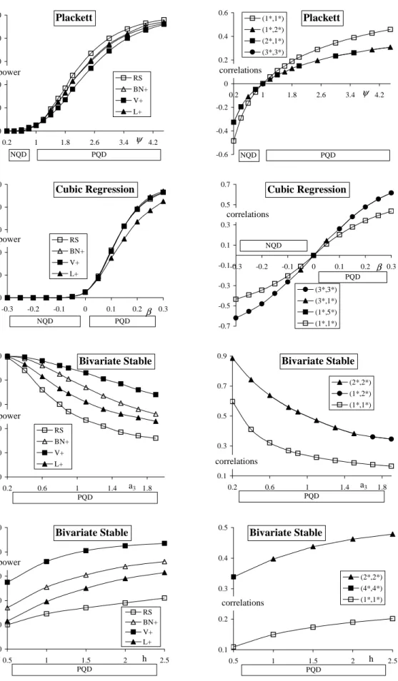
d1 Plackett (ψ). This family of distributions is nicely described on pages 191−197 of Johnson (1987). For ψ = 1 we have independence, ψ > 1 gives strictly P QD, while ψ<1corresponds to strictly negative quadrant dependence (N QD). Plackett noted the considerable similarity of his distribution with normal marginals to the usual bivariate normal distribution. Therefore, the usual bivariate normal distribution is not included for this testing problem. For the Plackett distributions thefirst correlationc∗
11is dominating, as is seen by(1∗,1∗) in Figure 1.
d2 Cubic regression model (β). Let X, Z be independent random variables each with a standard normal distribution and let
Y =βX3+Z.
For β = 0 we have independence, β >0 gives strictly P QD, while β <0 corresponds to strictly negative quadrant dependence. The correlation c∗33 is dominating, see (3∗,3∗) in Figure 1.
d3 Bivariate stable (a3). In general,(X, Y) has a bivariate stable distribution with para-meters(a1, a2, a3, b1, b2, b3, h) ifX =Z1+hZ3, Y =Z2+hZ3, h ∈R, whereZ1, Z2, Z3 are independent stable random variables,Zi ∼S(ai, bi), i= 1,2,3.In our application we used the parametrization of Chambers et al. (1976), page 341, and fixed a1 = 2, a2 = 0.2, b1 = 1, b2 =−1, b3 = 0, h= 1. Then for any a3 we have a strictlyP QD distribution. For these distributions the correlationc∗
0 20 40 60 80 100 0.2 1 1.8 2.6 3.4 4.2 RS BN+ V+ L+ Plackett power ψ NQD PQD -0.6 -0.4 -0.2 0 0.2 0.4 0.6 0.2 1 1.8 2.6 3.4 4.2 (1*,1*) (1*,2*) (2*,1*) (3*,3*) Plackett correlations ψ NQD PQD 0 20 40 60 80 100 0.2 0.6 1 1.4 1.8 RS BN+ V+ L+ Bivariate Stable power a3 PQD 0.1 0.3 0.5 0.7 0.9 0.2 0.6 1 1.4 1.8 (2*,2*) (1*,2*) (1*,1*) Bivariate Stable correlations a3 PQD 0.1 0.2 0.3 0.4 0.5 0.5 1 1.5 2 2.5 (2*,2*) (4*,4*) (1*,1*) Bivariate Stable correlations h PQD 0 20 40 60 80 100 -0.3 -0.2 -0.1 0 0.1 0.2 0.3 RS BN+ V+ L+ Cubic Regression power PQD NQD β -0.7 -0.5 -0.3 -0.1 0.1 0.3 0.5 0.7 -0.3 -0.2 -0.1 0 0.1 0.2 0.3 (3*,3*) (3*,1*) (1*,5*) (1*,1*) Cubic Regression correlations NQD PQD β 0 20 40 60 80 100 0.5 1 1.5 2 2.5 RS BN+ V+ L+ Bivariate Stable power h PQD
Figure 1. The simulated powers of 3 tests and the simulated correlation c∗11 together with the (next) most important simulated correlation c∗rs at distributions d1−d4.
d4 Bivariate stable (h) with a1 = 1.5, a2 = 0.1, a3 = 0.9, b1 = 1, b2 = −1, b3 = −0.5, h varying. When h= 0 we have independence, otherwise we get strictly P QD. Here the correlationc∗22 is dominating, see (2∗,2∗) in Figure 1.
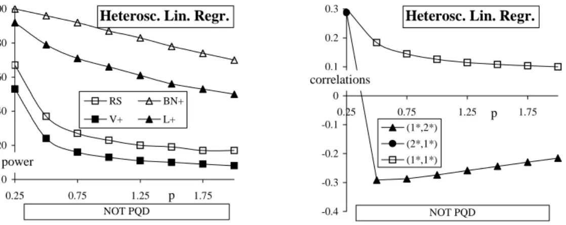
d5 Heteroscedastic linear regression(p). The distribution is obtained as follows. LetX be uniformly distributed at (0,1). Let Z be independent of X with a standard normal distribution. Then Y = X+ 4 (1−Xp) Z, where p > 0 varies. These distributions are notP QD. The dominating correlationc∗
12is negative, see(1∗,2∗)in Figure 2 (atp= 0.25 we have (1∗,2∗) =−0.236and(2∗,1∗) = 0.287).
The (simulated) powers of the three tests at the distributions d1−d4 are shown in Figure 1. Moreover, the simulated correlationc∗
11and the (next) most important simulated correlationc∗rs (amongc∗rs with r, s= 1, ...,5) of these distributions are also shown in Figure 1. For instance, in case of the Plackett distribution the most important (simulated) correlation (that is the one with the highest absolute value) among c∗rs with r, s= 1, ...,5 is c∗11= (1∗,1∗). The next most important one depends on the specific parameter value and is for example (1∗,2∗) atψ = 1.8, (2∗,1∗) atψ= 2, etc.
Sincec∗11is dominating for the Plackett alternatives, it is no surprise thatRShas the highest power for those alternatives. However, the differences are not that large. In the cubic regression model the three test have almost exactly the same power. It is clearly seen that for the bivariate stable alternatives with dominatingc∗22 great differences in power may occur. Although strictly P QD implies positive linear correlation, it is seen by the bivariate stable alternatives that V+ improves RS substantially when higher order correlations are exhibited by the data.
0 20 40 60 80 100 0.25 0.75 1.25 1.75 RS BN+ V+ L+
Heterosc. Lin. Regr.
power p NOT PQD -0.4 -0.3 -0.2 -0.1 0 0.1 0.2 0.3 0.25 0.75 1.25 1.75 (1*,2*) (2*,1*) (1*,1*)
Heterosc. Lin. Regr.
correlations
p
NOT PQD
Figure 2. The simulated powers of 3 tests and the simulated correlation c∗11 together with the (next) most important simulated correlation c∗
rs at distribution d5.
Figure 2 shows that BN+ and L+ have very high powers at the d5 distributions, although they are notP QD: at all presented parameter valuesp, except forp= 0.25the most important correlation, (1∗,2∗) is negative (at p = 0.25 we have (1∗,2∗) = −0.236 and (2∗,1∗) = 0.287). The other tests do not have such high power here, which we consider as an advantage, since the tests should concentrate as much as possible on positive dependence and not waste their power to distributions which are not P QD. Another advantage of V+ is that it is based on easily interpretable estimated grade correlations and additional inspection of these correlations can be helpful in situations when we are not sure that the data at hand obey theP QD pattern.
Remark 4.1We have also performed simulations forV+when d(n) = 3, see Remark 2.5. The simulated powers are as expected: some power loss when linear correlation is dominating and some gain otherwise.
In view of the results presented here and the other simulations that we have done we conclude that for testing independence against strictly P QD the new test based on V+performs very well for a wide variety of strictly P QD alternatives, going also behind the linear correlation.
4.2
Testing
P F D
When testing independence against strictlyP F D, we consider the following three test statistics. (a) Spearman’s rank correlation coefficient RS, see 4.1 (a).
(b) The new test statisticT+, see (9). (c) The new test statisticTo, see (10).
For all three test statistics we reject for large values of it. The simulations yield as critical values of T+ for n= 50 and level 0.05 : 2.81 ifd(50) = 1, 3.12 ifd(50) = 2,3.20if d(50) = 3, 3.24 if d(50) ≥ 4. The critical values of To for n = 50 and level 0.05 are: 2.81 if d(50) = 1, 3.97 if d(50) = 2, 4.15 if d(50) = 3, 4.21 if d(50) ≥ 4. This shows that for d(n) ≥ 2 there is almost no change in the critical values of T+ and To. This is a nice feature of these test statistics. Moreover, for data driven tests the power behavior is also very stable w.r.t. d(n), see e.g. Kallenberg and Ledwina (1997). Therefore, the problem of choosing kinTk+and Tko is definitely not replaced by the problem of choosing d(n). In the simulation study the testsT+ and To are applied with d(50) = 10.
SinceBN+is designed for testing independence against strictlyP QDwe do not present this test here. Anyway, we simulated the powers and they are high for most of these distributions as well, although for the alternatives d8 and d9 (see below) serious power loss w.r.tTo arises.
The following distributions are presented. The P F D-properties of these distributions are derived in the Appendix.
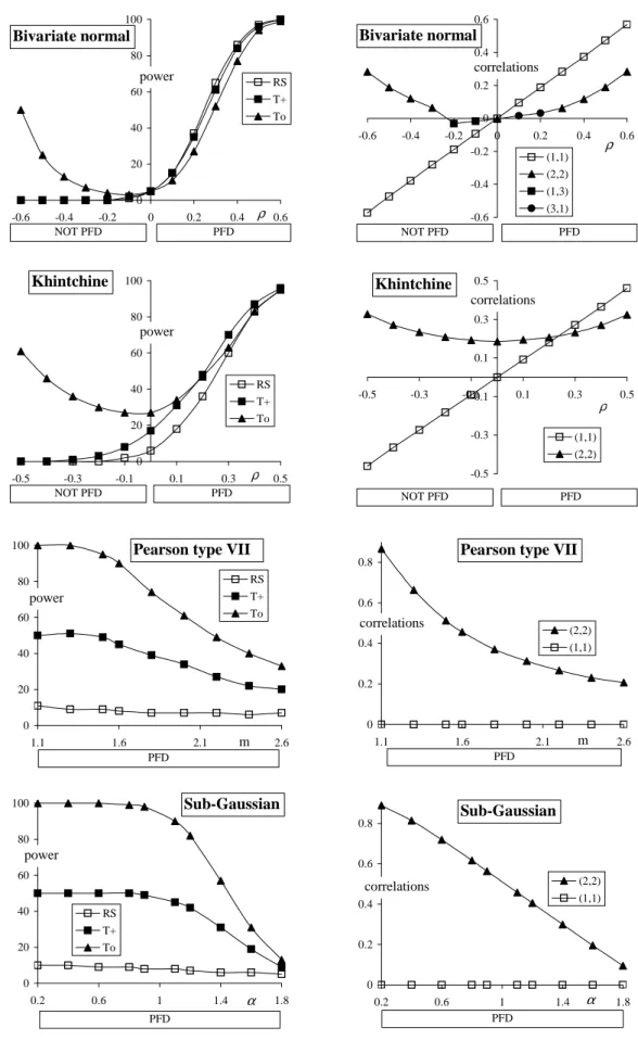
d6 Bivariate normal(ρ) with expectations equal to0, variances equal to1and correlation coefficient ρ. The bivariate normal distribution is strictly P F D for ρ>0, independence occurs for ρ = 0 and, remarkably (but see Remark 1.2), forρ < 0 we get neither P F D nor strictly negative function dependence. For the bivariate normal distributions the
first order correlation is dominating, as is seen by (1,1) in Figure 3, being positive for ρ > 0 and negative for ρ < 0, while the second order correlation, see (2,2), is positive for all ρ = 0 (for ρ = −0.2,−0.1 we get (2,2) = 0.029,0.007, respectively). Note that b2(x) = 6√5 x−12 2−12√5, see also Remark 1.2.
d7 Khintchine (ρ), defined as X = ZU, Y = ZV, where (U, V) has a bivariate normal distribution with expectations equal to0, variances equal to1 and correlation coefficient ρ, and Z being independent of (U, V), is distributed as χ2
3, where χ23 is a random variable with a chi-square distribution with 3 degrees of freedom. (This is not literally the Khintchine distribution, see e.g. Bryson and Johnson (1982), but a slight modification of it. Nevertheless we simply call it the Khintchine distribution.) The Khintchine (ρ) distributions withρ≥0are strictlyP F D, although forρ= 0the linear correlation equals 0, as is easily seen by symmetry arguments and independence of Z, U and V. For the Khintchine distributions with not too largeρ, the correlationc22 is dominating, while for
0 0.2 0.4 0.6 0.8 1.1 1.6 2.1 2.6 (2,2) (1,1) Pearson type VII
correlations m PFD 0 20 40 60 80 100 0.2 0.6 1 1.4 1.8 RS T+ To Sub-Gaussian power α PFD 0 0.2 0.4 0.6 0.8 0.2 0.6 1 1.4 1.8 (2,2) (1,1) Sub-Gaussian correlations α PFD 0 20 40 60 80 100 -0.6 -0.4 -0.2 0 0.2 0.4 0.6 RS T+ To Bivariate normal power ρ NOT PFD PFD -0.6 -0.4 -0.2 0 0.2 0.4 0.6 -0.6 -0.4 -0.2 0 0.2 0.4 0.6 (1,1) (2,2) (1,3) (3,1) Bivariate normal correlations ρ NOT PFD PFD -0.5 -0.3 -0.1 0.1 0.3 0.5 -0.5 -0.3 -0.1 0.1 0.3 0.5 (1,1) (2,2) Khintchine correlations ρ NOT PFD PFD 0 20 40 60 80 100 -0.5 -0.3 -0.1 0.1 0.3 0.5 RS T+ To Khintchine power ρ NOT PFD PFD 0 20 40 60 80 100 1.1 1.6 2.1 2.6 RS T+ To Pearson type VII
power
m PFD
Figure 3. The simulated powers of 3 tests and the simulated correlation c11 together with the
d8 Pearson type VII (m) withm >1, defined asX=U/√Z, Y =V /√Z, whereU, V and Z are independent random variables, U and V with a standard normal distribution and Z having a Gamma distribution with parameters(m−1,12). The Pearson type VII (m) distributions withm >1are strictlyP F D, although they have linear correlation equal to 0, as is easily seen by symmetry arguments. The correlationc22is dominating, see Figure 3.
d9 Sub-Gaussian (α). This subfamily of the sub-Gaussian distributions is defined asX = U√Z, Y =V√Z, whereU, V and Z are independent,U and V have a standard normal distribution and Z has a stable distribution, totally skewed to the right, with index of stability α/2, see Samorodnitsky and Taqqu (1994). The Sub-Gaussian (α) distributions are strictly P F D, although they have linear correlation equal to 0, as is easily seen by symmetry arguments. The correlationc22 is dominating, see Figure 3.
The (simulated) powers of the three tests at the distributions d6 −d9 are shown in Figure 3. Moreover, the simulated correlationc11and the (next) most important simulated correlation crs (amongcrs withr, s= 1, ...,10) of these distributions are also shown in Figure 3.
It is seen thatT+andToperform far much better thanRS, unless thefirst order correlation is dominating, as in the bivariate normal distribution (d6). A gain in power up to 90% for To is seen in d8 and d9! On the other hand, the loss in power at alternatives with dominatingfirst order correlation is not very large. As explained in Section 3 when introducing T+, in case of a linear correlation equal to 0 its asymptotic power is at most 12. This is clearly shown at the alternatives d8 and d9: while for small parameter values the power ofTo comes close to 100%, the power ofT+ reaches 50%.
The asymptotic null distribution of T+ and To and the consistency of the tests based on T+ andTo for a very large class of positive dependent alternatives are shown in the Appendix. Although formally T+ is not consistent when the linear correlation equals 0, the alternatives d7 − d9 show that a substantial power gain w.r.t. Spearman’s rank correlation test can be obtained when the linear correlation is (close to)0. To facilitate their application a simple, but accurate approximation for the critical values and/or p-values of T+ and To is given as well in the Appendix.
It is seen in the bivariate normal distribution (d6) that To may have substantial power at distributions which are not P F D. In that case the power comes from the fact that the correlationc22 is positive. For instance, whenρ=−0.6 we getc22 = 0.28, see Figure 3. This agrees with the consistency result (Theorem 2 in the Appendix), which states that the test based onTo is consistent against any alternative with positivecjj for some j. In this sense the test statistic To is liberal, which is no problem as long as we consider distributions that are either independent or strictlyP F D.
In view of the results presented here and the other simulations that we have done we conclude that for testing independence against strictly P F D the new tests based on T+ and To are useful
and flexible tools to detect P F D alternatives, going also behind linear correlation.
Remark 4.2 All three tests V+, T+ and To are expected to have higher power than the corresponding unrestricted tests V and T S2 in Kallenberg and Ledwina (1999), since V+,T+ and To are tuned to distributions with positive dependence. Indeed, in our simulation study this clearly comes up. For instance, at each of the alternatives d1 − d4 the power of V+ is about0.20higher than the power ofV for parameter values such that the power is not too high
or too low. So, the gain of concentrating onP QD alternatives (V+) or P F D alternatives (T+ and To) is pretty much.
Appendix
In this appendix we give details about the projected Legendre polynomials, the distribu-tions used in the simulation study and further we present here some theoretical properties of T+andTo, their asymptotic null distribution and their consistency. Moreover, we give an easy, but accurate approximation for the critical values and/or p-values of T+ andTo.
Projected Legendre polynomials
The first five projected Legendre polynomials on the space of nondecreasing functions, nor-malized such that
1 0 {b∗i(u)}2du= 1, i= 1,2, ..., are given by b∗1(u) = b1(u) = √ 3(2u−1) = 3.4641u−1.7321; b∗2(u) = − √ 10 √ 47I 0≤u≤ 3 4 + 8√2 √ 47b2(u)I 3 4 < u≤1 = −0.4613I{0≤u≤0.75}+ 1.6503b2(u) I{0.75< u≤1}; b∗3(u) = b3(u) 1−18 √ 15 10 I 0≤u≤ 1 2 − √ 15 10 +I 1 2 + √ 15 10 ≤u≤1 = 1.2262 b3(u) [I{0≤u≤0.1127}+I{0.8873≤u≤1}] ; b∗4(u) = −0.8387I{0≤u≤0.2950}+ 2.1219b4(u)I{0.2950< u≤0.3348} +0.1137I{0.3348< u≤0.9324}+ 2.1219b4(u)I{0.9324< u≤1}; b∗5(u) = 1.8625 b5(u)I{0≤u≤0.0452}−0.1476I{0.0452< u≤0.4936} +1.8625b5(u)I{0.4936< u≤0.5064}+ 0.1476I{0.5064< u≤0.9548} +1.8625b5(u)I{0.9548< u≤1}. Verification P QD
d1 Plackett(ψ). By direct calculation from the distribution function as given on page192in Johnson (1987) it is easily verified that we have strictlyP QD when ψ>1, independence when ψ= 1and strictly negative quadrant dependence when ψ<1.
d2 Cubic regression model(β). It follows immediately from Example 1 (iv) in Lehmann (1966) that forβ >0we getP QDand, similarly, forβ<0negative quadrant dependence. Moreover, cov(X, Y) = 0 when β = 0 and hence we have strictly P QD for β > 0 and strictly negative quadrant dependence forβ<0. By definition ofY, we have independence when β= 0.
d3 Bivariate stable(a3)with further thefixed valuesa1= 2, a2 = 0.2, b1 = 1, b2 =−1, b3 = 0, h = 1. This distribution is of the form X =Z1+hZ3, Y = Z2+hZ3 with Z1, Z2, Z3
independent random variables. By Example 1 (ii) in Lehmann (1966) it follows that the bivariate stable distribution isP QD. Whenh= 0, obviously we have independence. Since cov(X, Y) > 0 when h= 0, we conclude that the bivariate stable distribution is strictly P QD forh= 0.
d4 Bivariate stable (h) with a1 = 1.5, a2 = 0.1, a3 = 0.9, b1 = 1, b2 = −1, b3 =−0.5. See d3.
d5 Heteroscedastic linear regression(p). As remarked before these distributions are not P QD.
Verification P F D
d6 Bivariate normal(ρ) with expectations equal to 0, variances equal to1and correlation coefficient ρ. For ρ ≥ 0 the bivariate normal is a prominent example of distributions with a diagonal expansion, called P DE in Shaked (1979), page 69. On page 70 Shaked shows that each P DE is positive definite dependent (P DD), which in turn is equivalent toP F D, see Proposition 2.2 in Shaked (1979). Obviously, this concerns forρ>0strictly P F D, since cov(X, Y) > 0. For ρ = 0 we have independence. For ρ < 0 we do not get strictly negative function dependence, but neither P F D (since c11<0) nor negative function dependence (sincec22>0).
d7 Khintchine (ρ) is defined as X = ZU, Y = ZV, where (U, V) has a bivariate normal with expectations equal to 0, variances equal to 1 and correlation coefficient ρ and Z being independent of(U, V)is distributed as χ23. It follows from Theorem 3.1 in Shaked (1979) with (X1, Y1) = (U, V),(X2, Y2) = (Z, Z) and h(x, y) = xy that Khintchine (ρ) withρ≥0 is P F D. Furthermore, usingE U2V2 = 1 + 2ρ2 ≥1, we getcov(X2, Y2) = EZ4E U2V2 − EZ2 2 ≥var(Z2)>0 and hence we have strictlyP F D.
d8 Pearson type VII (m) is defined as X = U/√Z, Y = V /√Z, where U, V and Z are independent random variables,U andV with a standard normal distribution andZ having a Gamma distribution with parameters(m−1,12). Hence, by Proposition 2.1 in Shaked (1979) it is seen that this distribution is positively dependent by mixture, which implies P F D, see page 70 in Shaked (1979). Lett >0be such thatE √1
Z 2t <∞. Then we get cov(|X|t,|Y|t) =var √1 Z t
E|U|tE|V|t>0and hence we have strictly P F D. d9 Sub-Gaussian (α) is defined as X = U√Z, Y = V√Z, where U, V and Z are
inde-pendent, U and V have a standard normal distribution and Z has a stable distribution, totally skewed to the right, with index of stability α/2. By Proposition 2.1 in Shaked (1979) it is seen that this distribution is positively dependent by mixture, which implies P F D, see page 70 in Shaked (1979). Let t >0 be such thatE √Z 2t <∞. Then we getcov(|X|t,|Y|t) =var √Z t E|U|tE|V|t>0 and hence we have strictlyP F D.
Asymptotic null distribution T+ and To As defined in (6), we have (C1, ..., Ck) = 1 √ n n i=1 b1 Ri− 12 n b1 Si−12 n , ..., n i=1 bk Ri−12 n bk Si−12 n .
The derivations of the asymptotic null distributions of T+ and To go along the same lines of argument. As might be expected the selection rule concentrates on dimension1underH0. Since T+ and To are the same when restricted to dimension 1, we get the same asymptotic result for T+ and To. Furthermore, to prove that the selection rule concentrates on dimension 1, it is enough to know that they are dominated by kj=1C2
j. To show that this is indeed essential and doing so making the proof more transparent, we therefore derive at once the asymptotic null distribution for the whole class of tests statistics with these features, defined as
ˇ
TSˇ with0≤Tˇk≤ k
j=1
Cj2 and Tˇ1 =C12I(C1 >0),
whereSˇ= min k: 1≤k≤d(n) :Tˇk−klogn≥Tˇr−rlogn,1≤r≤d(n) . Note thatT+ and To belong to this class.
Theorem 1 Assume that H0 is true and denote the probability measure under H0 by P0. If d(n) =o {n/logn}101 , then for every test statistic
ˇ
TSˇ with 0≤Tˇk ≤ k
j=1
Cj2 and Tˇ1 =C12I(C1>0),
whereSˇ= min k: 1≤k≤d(n) :Tˇk−klogn≥Tˇr−rlogn,1≤r≤d(n) ,
we have lim n→∞P0( ˇ S = 1) = 1and lim n→∞P0 ˇ TSˇ ≤x = Φ(√x) if x≥0 0 if x <0 , (11)
whereΦdenotes the standard normal distribution function. Note thatlimn→∞P0 TˇSˇ= 0 = 12.
Proof. The proof of Theorem 1 follows from the proof of Theorem 1 in Kallenberg and Ledwina (1999). By definition of Sˇand the assumption 0≤Tˇk ≤ kj=1Cj2 we get
P0(Sˇ ≥ 2) = d(n) k=2 P0(Sˇ=k)≤ d(n) k=2 P0 Tˇk≥(k−1) logn ≤ d(n) k=2 P0 k j=1 Cj2 ≥(k−1) logn .
Application of (A.1) and (A.2) on page 297 in Kallenberg and Ledwina (1999) gives
lim n→∞ d(n) k=2 P0 k j=1 Cj2≥(k−1) logn = 0,
implying lim n→∞P0( ˇ S = 1) = 1. (12) Using P0 TˇSˇ ≤x = P0 Tˇ1 ≤x,Sˇ= 1 +P0 TˇSˇ≤x,Sˇ≥2 = P0 Tˇ1 ≤x −P0 Tˇ1 ≤x,Sˇ≥2 +P0 TˇSˇ≤x,Sˇ≥2 ,
the limiting distribution of TˇSˇ under H0 immediately follows from (12), the assumption Tˇ1 = C12I(C1 >0)and the asymptotic standard normality of C1 underH0.
Consistency of To
The consistency of To is presented in the following theorem.
Theorem 2 Let Pbe an alternative and let F and G be the marginal distribution functions of
X andY, respectively under P. Let
cjj =EPbj(F(X))bj(G(Y))>0 (13)
for some j. If d(n) tends to infinity andd(n) =o {n/logn}101 , thenTo is consistent against
P.
Proof. By (A.11) and (A.12) on page 299 in Kallenberg and Ledwina (1999) we have for any r, s, 1 n n i=1 br Ri−12 n bs Si−12 n P →EPbr(F(X))bs(G(Y)) (14)
asn→ ∞. LetJ be the smallestj≥1for which (13) holds. LetCj be defined as in (6). In view of (14) we get for anyj ∈{1, ..., J−1} thatI(Cj >0)→P 0 ifEPbj(F(X))bj(G(Y))<0 and n−1Cj2 →P 0 if EPbj(F(X))bj(G(Y)) = 0. Hence, n−1Tjo
P
→ 0 for any j ∈ {1, ..., J −1}. Moreover, I(CJ >0) →P 1, n−1CJ2 →P {EPbJ(F(X))bJ(G(Y))}2 > 0, implying n−1TJo →P
{EPbJ(F(X))bJ(G(Y))}2 > 0. Because d(n) → ∞, we have d(n) ≥ J for all sufficiently largen. For anyj∈{1, ..., J−1}, the foregoing implies
n−1Tjo−jn−1logn < n−1TJo−Jn−1logn
for all sufficiently large n and hence, P(S2o=j) →P 0 for any j ∈{1, ..., J−1} and therefore, P(S2o ≥J)→P 1.
For any j≥J, it follows from (7) thatTjo≥TJo. Noting thatTJo → ∞P andP(S2o≥J)→P 1 we also getTo→ ∞P . By Theorem 1 the proof of Theorem 2 is complete.
The class of positive dependent alternatives for which consistency ofTo holds is rather large. In particular, for any strictly P QD alternative P the linear correlation is strictly positive, cf. Remark 2.4, and hence, by Theorem 2,Tois consistent against any strictlyP QDalternative. For any strictlyP F D alternative P we havecovP(f(F(X)), f(G(Y)))≥0 for allf with inequality for at least somef, implyingEPbj(F(X))bj(G(Y))≥0for allj. As a rule, for a strictlyP F D alternative we will have inequality for somej and hence consistency ofTo.
Consistency of T+
The consistency ofT+ is presented in the following theorem. Noting thatT+ ≥T+
1 allows to pattern the proof of Theorem 2. We omit the details.
Theorem 3 Let Pbe an alternative and let F and G be the marginal distribution functions of
X andY, respectively under P. Let c11=EPb1(F(X))b1(G(Y))>0. Ifd(n) tends to infinity
and d(n) =o {n/logn}101 , thenT+ is consistent against P.
The test based onT+ is consistent against any alternativePfor which the linear correlation EPb1(F(X))b1(G(Y))>0 and hence in particular for any strictly P QD alternative, cf. Re-mark 2.4. That T+ is not consistent at strictlyP F D alternatives with linear correlation equal to0 was already discussed when introducingT+ in Section 3.
Approximation for critical values and p-values
The first order approximations of To and T+ given in (11) is not very accurate. For in-stance the simulated critical values for n = 50, d(n) ≥ 4 and α = 0.05 equal 3.24 and 4.21, respectively, while the approximation based on Theorem 1 yields 2.71. The same phenomenon occurs in data driven tests for other testing problems like testing goodness offit. The remedy is a second order approximation following the line of argument given by Kallenberg and Ledwina (1995, Section 4).
The idea is that To ≥ T1o = C121 (C1 >0) and T+ ≥ T1+ = C121 (C1 >0), implying that P(To≤x) and P(T+≤x) are underestimated by the first order approximation Φ(√x). We apply the following approximations (we denote by =. approximately equals to)
P(To ≤x)=. P(T1o ≤x, S2 = 1) +P(T2o≤x, S2 = 2) . = P(T1o ≤x)−P(T1o ≤x≤T2o, S2 = 2) . = P C1 ≤ √ x −P (C1I{C1>0})2 ≤x≤(C1I{C1>0})2+ (C2I{C2>0})2,(C2I{C2>0})2 >logn . ReplacingC1 and C2 by (independent)N(0,1)-distributed random variables, a further approx-imation leads to thefinal proposal
P(To ≤x)=. Φ(√x)Φ √logn ifx≤logn Φ(√x)−12Φ(−√x)−e −x/2 4 ifx≥2 logn
linearize if logn < x <2 logn.
(15)
Inserting the simulated critical value4.21forn= 50andα= 0.05 in (15) gives0.956, which is rather close to0.95and a big improvement compared to the approximation based on Theorem 1, yielding Φ √4.21 = 0.980. Similarly we get P T+≤x =.
Φ(√x)Φ √logn +21Φ −√logn ifx≤logn Φ(√x)− e
−x/2
4 ifx≥2 logn
linearize if logn < x <2 logn.
(16)
Inserting the simulated critical value3.24forn= 50andα= 0.05 in (16) gives0.953, which is rather close to0.95 and an improvement compared to the approximation based on Theorem 1, yielding Φ √3.24 = 0.964.
References
Albers, W. (1999). Stop-loss premiums under dependence. Insurance Math. Econom. 24 173-185.
Albers, W., Kallenberg, W.C.M. and Martini, F. (2001). Data driven rank tests for classes of tail alternatives. J. Amer. Statist. Assoc. 96685-696.
Behnen, K. and Neuhaus, G. (1989). Rank Tests with Estimated Scores and Their Applica-tion. Teubner, Stuttgart.
Breiman (1968). Probability, Addison-Wesley, Reading, Massachusetts.
Bryson, M.C. and Johnson, M.E. (1982). Constructing and simulating multivariate distrib-utions using Khintchine’s theorem. J. Statist. Comput. Simul. 16129-137.
Chambers, J.M., Mallows, C.L. and Stuck, B.W. (1976). A method for simulating stable random variables. J. Amer. Statist. Assoc. 71340-344.
Denuit, M. , Dhaene, J. and Ribas, C. (2001). Does positive dependence between individual risks increase stop-loss premiums? Insurance Math. Econom. 28305-308.
Embrechts, P., McNeil, A. and Straumann, D. (2002). Correlation and dependency in risk management: properties and pitfalls. In: Risk Management: Value at Risk and Beyond (Eds. Dempster, M. and Moffatt, H.). Cambridge University Press, Cambridge, pp. 176-223.
Esary, J.D., Proschan, F. and Walkup, D.W. (1967). Association of random variables, with applications. Ann. Math. Statist. 381466-1474.
Joe, H. (1997). Multivariate Models and Dependence Concepts. Chapman & Hall, London. Johnson, M.E. (1987)Multivariate Statistical Simulation. Wiley, New York.
Kallenberg, W.C.M. and Ledwina, T. (1995). On data driven Neyman’s tests. Probab. Math. Statist. 15 409-426.
Kallenberg, W.C.M. and Ledwina, T. (1997). Data-driven smooth tests when the hypothesis is composite. J. Amer. Statist. Assoc. 92 1094-1104.
Kallenberg, W.C.M. and Ledwina, T. (1999). Data-driven rank tests for independence. J. Amer. Statist. Assoc. 94285-301.
Kowalczyk,T. and Pleszczy´nska, E. (1977). Monotonic dependence functions of bivariate distributions. Ann. Statist. 51221-1227.
Ledwina, T. (1986). Large deviations and Bahadur slopes of some rank tests of indepen-dence. Sankhy¯a A48188-207.
Ledwina, T. (1994). Data driven version of Neyman’s smooth test of fit. J. Amer. Statist. Assoc. 891000-1005.
Lehmann, E. (1966). Some concepts of dependence. Ann. Math. Statist. 371137-1153. Mari, D.D. and Kotz, S. (2001). Correlation and Dependence. Imperial College Press, London.
Metry, M.H. and Sampson, A.R. (1991). A family of partial orderings for positive depen-dence among fixed marginal bivariate distributions. In: Advances in Probability Distributions with Given Marginals : Beyond the Copulas (Eds. G. Dall’ Aglio, S. Kotz and G. Salinetti). Kluwer, Dordrecht, Netherlands, pp. 129-138.
Rychlik, T. (2001)Projecting Statistical Functionals. Lecture Notes in Statistics 160, Springer, New York.
Samorodnitsky, G. and Taqqu, M.S. (1994). Stable Non-Gaussian Random Processes: Sto-chastic Models With Infinite Variance, New York, Chapman and Hall.
Scarsini, M. and Shaked, M. (1996). Positive dependence orders: a survey. In: Athens Conference on Applied Probability and Time Series I: Applied Probability (Eds. C.C. Heyde, Yu V. Prohorov, R. Pyke and S.T. Rachev). Springer, New York, pp. 70-91.
Schriever, B.F. (1987). An ordering of positive dependence. Ann. Statist. 151208-1214. Schwarz, G. (1978). Estimating the dimension of a model. Ann. Statist. 6461-464.
Shaked, M. (1979). Some concepts of positive dependence for bivariate interchangeable distributions. Ann. Inst. Statist. Math. 3167-84.
Thas, O. (2001). Nonparametrical tests based on sample space partitions. PhD Dissertation, University of Gent.