On the numerical analysis of eigenvalue problems

D I S S E R T A T I O N

zur Erlangung des akademischen Grades

Dr. rer. nat.

im Fach Mathematik

eingereicht an der

Mathematisch-Naturwissenschaftlichen Fakultät II

Humboldt-Universität zu Berlin

von

Dipl.-Math. Joscha Micha Gedicke

Präsident der Humboldt-Universität zu Berlin:

Prof. Dr. Jan-Hendrik Olbertz

Dekan der Mathematisch-Naturwissenschaftlichen Fakultät II:

Prof. Dr. Elmar Kulke

Gutachter:

1. Prof. Dr. Carsten Carstensen

2. Prof. Dr. Volker Mehrmann

3. Prof. Dr. Rolf Rannacher

Vielen Dank an Herrn Prof. V. Mehrmann und Frau Dr. A. Miedlar für die erfolg-reiche Zusammenarbeit im MATHEON Forschungsprojekt C22 “Adaptive solutions of parametric eigenvalue problems”.

Vielen Dank auch an die gesamte Arbeitsgruppe “Numerical Analysis” von Herrn Prof. C. Carstensen für die sehr angenehme Arbeitsatmosphäre.

Nicht zuletzt vielen Dank an das MATHEON und die BMS für die finanzielle Unter-stützung meiner Promotion.

Ich widme diese Arbeit meinen Eltern und meiner Schwester.

This thesis “on the numerical analysis of eigenvalue problems” consists of five major aspects of the numerical analysis of adaptive finite element methods for eigenvalue problems. The first three consider the symmetric Laplace eigenvalue problem while the last two concern a non-symmetric convection-diffusion eigen-value problem.

The first part presents a combined adaptive finite element method with an iterative algebraic eigenvalue solver for a symmetric eigenvalue problem of asymp-totic quasi-optimal computational complexity. The analysis is based on a direct approach for eigenvalue problems and allows the use of higher-order conforming finite element spaces with fixed polynomial degree. The asymptotic quasi-optimal adaptive finite element eigenvalue solver involves a proper termination criterion for the algebraic eigenvalue solver and does not need any coarsening. Numerical evidence illustrates the asymptotic quasi-optimal computational complexity in 2 and 3 dimensions.

The second part introduces fully computable two-sided bounds on the eigenval-ues of the Laplace operator on arbitrarily coarse meshes based on some approxi-mation of the corresponding eigenfunction in the nonconforming Crouzeix-Raviart finite element space plus some postprocessing. The efficiency of the guaranteed error bounds involves the global mesh-size and is proven for the large class of graded meshes. Numerical examples demonstrate the reliability of the guaranteed error control even for coarse meshes and inexact solve of the algebraic eigenvalue problem. This motivates an adaptive algorithm which monitors the discretisation error, the maximal mesh-size, and the algebraic eigenvalue error. The accuracy of the guaranteed eigenvalue bounds is surprisingly high with efficiency indices as small as 1.4.

The third part presents an adaptive finite element method (AFEM) based on nodal-patch refinement that leads to an asymptotic error reduction property for the adaptive sequence of simple eigenvalues and eigenfunctions of the Laplace operator. The proven saturation property yields reliability and efficiency for a class of hierarchical a posteriori error estimators. Numerical experiments confirm that the saturation property is present even for very coarse meshes for many examples, but in other cases the smallness assumption on the initial mesh is severe.

The fourth part considers a posteriori error estimators for convection-diffusion eigenvalue problems as discussed by Heuveline and Rannacher (2001) in the context of the dual-weighted residual method (DWR). This presentation directly addresses the variational formulation rather than the non-linear ansatz of Becker and Ran-nacher. Two different postprocessing techniques attached to the DWR paradigm plus two new dual-weighted a posteriori error estimators are presented. The first new estimator utilises an auxiliary Raviart-Thomas mixed finite element method and the second exploits an averaging technique in combination with ideas of DWR. The six a posteriori error estimators compete in three numerical examples and il-lustrate reliability and efficiency and the dependence of generic constants on the size of the eigenvalue or the convection coefficient.

veloped algorithms is a homotopy method which departs from a well-understood selfadjoint problem. Apart from the adaptive grid refinement, the progress of the homotopy as well as the solution of the iterative method are adapted to balance the contributions of the different error sources. The first algorithm balances the homotopy, discretisation and approximation errors with respect to a fixed step-size in the homotopy. The second algorithm combines the adaptive step-size control for the homotopy with an adaptation in space that ensures an error below a fixed tolerance. The outcome leads to the third algorithm which allows the complete adaptivity in space, homotopy step-size as well as the iterative algebraic eigenvalue solver. All three algorithms compete in numerical examples.

Die vorliegende Arbeit zum Thema der numerischen Analysis von Eigenwertpro-blemen befasst sich mit fünf wesentlichen Aspekten der numerischen Analysis von Eigenwertproblemen. Die ersten drei befassen sich mit dem symmetrischen Laplace Eigenwertproblem wohingegen sich die letzten beiden mit einem unsymmetrischen Konvektion-Diffusion Eigenwertproblem beschäftigen.

Der erste Teil präsentiert einen Algorithmus, der die adaptive Finite Elemente Methode mit einem iterativen algebraischen Eigenwertlöser kombiniert. Es wird gezeigt, dass dieser Algorithmus asymptotisch quasi-optimale Rechenlaufzeit be-sitzt. Die Analysis basiert auf einem direkten Ansatz für das Eigenwertproblem. Sie gilt für konforme Finite Elemente höherer Ordnung mit festem Polynomgrad. Der asymptotisch quasi-optimale adaptive Finite Elemente Eigenwertlöser beinhaltet ein Kriterium zum rechtzeitigen Stoppen der Iterationen und braucht keine Vergrö-berungen der Gitter. Numerische Experimente demonstrieren die quasi-optimalen Laufzeiten in zwei und drei Raum-Dimensionen.

Der zweite Teil präsentiert explizite beidseitige Schranken für die Eigenwerte des Laplace Operators auf beliebig groben Gittern basierend auf einer Approxi-mation der zugehörigen Eigenfunktion in dem nicht konformen Finite Elemente Raum von Crouzeix und Raviart und einem Postprocessing. Die Effizienz der ga-rantierten Schranke des Eigenwertfehlers hängt von der globalen Gitterweite ab. Trotzdem kann sie hier für die große Klasse von graduierten Gittern bewiesen werden. Numerische Experimente zeigen die Zuverlässigkeit der garantierten Feh-lerkontrolle sogar für inexakte algebraische Näherungen der Eigenfunktionen. Dies motiviert einen adaptiven Algorithmus der den Diskretisierungsfehler, die globa-le Gitterweite und den algebraischen Fehgloba-ler kontrolliert und ausbalanciert. Die Genauigkeit der garantierten Eigenwert-Schranken ist überraschend sehr gut mit Effizienz-Indizes von 1.4.

Der dritte Teil betrachtet eine adaptive Finite Elemente Methode basierend auf Verfeinerungen von Knoten-Patchen. Dieser Algorithmus zeigt eine asymptotische Fehlerreduktion der adaptiven Sequenz von einfachen Eigenwerten und Eigenfunk-tionen des Laplace Operators. Die hier erstmals bewiesene Eigenschaft der Satu-ration des Eigenwertfehlers zeigt Zuverlässigkeit und Effizienz für eine Klasse von hierarchischen a posteriori Fehlerschätzern. Numerische Experimente verifizieren, dass die Saturations-Eigenschaft in vielen Benchmarks selbst auf sehr groben Git-tern gilt. In manchen gezeigten Experimenten ist die Annahme, dass die globale Gitterweite hinreichen klein ist, jedoch kritisch.

Der vierte Teil betrachtet a posteriori Fehlerschätzer für Konvektion-Diffusion Eigenwertprobleme, wie sie von Heuveline und Rannacher (2001) im Kontext der dual-gewichteten residualen Methode (DWR) diskutiert wurden. Im Gegensatz zum nicht linearen Ansatz von Becker und Rannacher wird hier ein direkter An-satz für die Variationsformulierung vorgestellt. Zwei verschiedene Techniken für das Postprocessing im Kontext der DWR Methode und zusätzlich zwei neue dual-gewichtete a posteriori Fehlerschätzer werden vorgestellt. Der erste neue Fehler-schätzer benutzt eine zusätzliche Raviart-Thomas gemischte Finite Elemente

Lö-rischen Benchmarks verglichen und auf Zuverlässigkeit und Effizienz hin unter-sucht. Die numerischen Experimente zeigen die Abhängigkeit der Fehlerschranken von generischen Konstanten, der Größe des Eigenwertes oder dem Konvektion-Koeffizienten.

Der letzte Teil beschäftigt sich mit drei adaptiven Algorithmen für Eigenwertpro-bleme von nicht selbst-adjungierten Operatoren partieller Differentialgleichungen. Alle drei Algorithmen basieren auf einer Homotopie-Methode die vom einfache-ren selbst-adjungierten Problem startet. Neben der Gitterverfeinerung wird der Prozess der Homotopie sowie die Anzahl der Iterationen des algebraischen Löser adaptiv gesteuert und die verschiedenen Anteile am gesamten Fehler ausbalan-ciert. Der erste Algorithmus zeigt Methoden zum Ausbalancieren der Fehler der Homotopie, der Diskretisierung und der algebraischen Approximation für eine fes-te Schrittweifes-te der Homotopie. Der zweifes-te Algorithmus kombiniert eine adaptive Steuerung der Schrittweiten der Homotopie mit der adaptiven Finiten Elemente Methode im Raum mittels einer festen Fehlertoleranz. Die Kombination beider Algorithmen führt auf den dritten Algorithmus der die Vorteile der ersten bei-den kombiniert und damit komplett adaptiv in allen drei Richtungen, dem Raum, der Homotopie, und den algebraischen Iterationen, adaptive arbeitet. Alle drei Algorithmen werden in numerischen Benchmarks miteinander verglichen.

1 Introduction 1

1.1 Motivation . . . 1

1.2 State of the Art . . . 2

1.3 Overview and Main Results . . . 3

1.4 Outlook and Open Questions . . . 10

2 Preliminaries 12 2.1 Functional Analysis Background . . . 12

2.2 Finite Elements . . . 14

2.2.1 Conforming Finite Element . . . 15

2.2.2 Nonconforming Finite Element . . . 15

2.3 The Symmetric Model Eigenvalue Problem . . . 16

2.3.1 Conforming Discrete Eigenvalue Problem . . . 16

2.3.2 Nonconforming Discrete Eigenvalue Problem . . . 17

2.4 The Non-Symmetric Model Eigenvalue Problem . . . 18

2.5 Adaptive Mesh-Refinement Algorithms . . . 19

2.5.1 Closure Algorithm . . . 20

2.5.2 Red-Green-Blue Refinement . . . 20

2.5.3 Newest-Vertex Bisection . . . 20

3 An AFEMES of Asymptotic Quasi-Optimal Complexity 22 3.1 Introduction . . . 22

3.2 Adaptive Finite Element Eigenvalue Solver . . . 25

3.2.1 Solve . . . 25

3.2.2 Estimate . . . 26

3.2.3 Mark . . . 26

3.2.4 Refine . . . 27

3.3 Algebraic Properties . . . 27

3.4 A Posteriori Error Estimator . . . 30

3.5 Quasi-Optimal Convergence . . . 33

3.6 Quasi-Optimal Convergence for Inexact Algebraic Solutions . . . 36

3.7 Quasi-Optimal Complexity . . . 41 3.8 Numerical Experiments . . . 43 3.8.1 Slit Domain . . . 43 3.8.2 Unit Cube . . . 47 3.8.3 3D L-Shaped Domain . . . 48 3.9 Software Implementation . . . 51

4 Guaranteed Lower Bounds for Eigenvalues 55

4.1 Introduction . . . 55

4.2 Notation and Preliminaries . . . 57

4.3 Explicit Bounds for the Smallest Eigenvalue . . . 59

4.4 Efficiency for Graded Meshes . . . 65

4.5 Error Bounds for Higher Eigenvalues . . . 70

4.6 Numerical Experiments . . . 74

4.6.1 Adaptive Finite Element Algorithm . . . 74

4.6.2 Unit Square . . . 76

4.6.3 L-Shaped Domain . . . 77

4.6.4 Isospectral Domains . . . 79

4.7 Software Implementation . . . 79

5 AFEM Saturation for EVPs 83 5.1 Introduction . . . 83

5.2 Adaptive Finite Element Method . . . 84

5.2.1 Solve . . . 85 5.2.2 Estimate . . . 86 5.2.3 Mark . . . 86 5.2.4 Refine . . . 86 5.3 Discrete Efficiency . . . 87 5.4 Saturation Property . . . 90 5.5 Numerical Examples . . . 93 5.5.1 Preliminary Remarks . . . 93 5.5.2 Unit Square . . . 94 5.5.3 L-Shaped Domain . . . 94 5.5.4 Isospectral Domains . . . 94

5.5.5 Three hierarchical adaptive algorithms . . . 97

5.5.6 Conclusions . . . 99

5.6 Software Implementation . . . 100

6 A Posteriori Error Estimators for Convection-Diffusion EVPs 103 6.1 Introduction . . . 103

6.2 Algebraic Properties . . . 105

6.3 A Posteriori Error Estimates . . . 108

6.3.1 Residual Estimator . . . 109 6.3.2 Averaging Estimator . . . 110 6.3.3 DWR1 Estimator . . . 111 6.3.4 DWR2 Estimator . . . 113 6.3.5 DWM Estimator . . . 113 6.3.6 DWA Estimator . . . 114

6.4 Adaptive Finite Element Method . . . 115

6.4.1 Solve . . . 115

6.4.3 Mark . . . 119 6.4.4 Refine . . . 119 6.5 Numerical Experiments . . . 119 6.5.1 Unit Square . . . 119 6.5.2 L-Shaped Domain . . . 122 6.5.3 Slit Domain . . . 125 6.6 Conclusions . . . 125 6.7 Software Implementation . . . 128

7 Adaptive Homotopy Methods 131 7.1 Introduction . . . 131

7.2 Adaptive Finite Element Methods . . . 133

7.2.1 Solve . . . 134 7.2.2 Estimate . . . 134 7.2.3 Mark . . . 135 7.2.4 Refine . . . 135 7.3 Homotopy Methods . . . 135 7.4 Homotopy Error . . . 136

7.5 A Posteriori Error Estimator . . . 137

7.6 Algorithms . . . 140 7.6.1 Algorithm 1 . . . 142 7.6.2 Algorithm 2 . . . 143 7.6.3 Algorithm 3 . . . 145 7.7 Numerical Experiments . . . 146 7.7.1 Example 1 . . . 149 7.7.2 Example 2 . . . 151 7.7.3 Example 3 . . . 151 7.8 Software Implementation . . . 154 Bibliography 158 List of Figures 166 List of Tables 169 Selbständigkeitserklärung 170

The computation of eigenvalues is a fundamental task of numerical mathematics and arises in a large variety of important applications in science and engineering: Eigenvalue problems occur in the dynamics of elastic bodies, the vibrations of membranes, in the separation of variables ansatz for the problems of heat conduction or acoustics, or in the hydrodynamic stability analysis.

1.1 Motivation

For a motivation of this thesis three generally understandable examples for the relevance of eigenvalues/frequencies or eigenfunctions/modes are presented in the following.

The first example is the probably most famous example of structural failure of the Tacoma Narrows bridge in 1940 due to too large vibrations of some fundamental mode of the bridge. This mode was some lower torsional twisting vibration mode that had never been observed before. The forces of the wind caused this natural mode of the bridge to vibrate [18] – this physical effect is called aeroelastic fluttering. The enforced vibration of the Tacoma Narrows bridge was a self-exciting vibration that finally caused its failure. Engineers investigated the vibrations of the “Galloping Gerti” and filmed its final damage. Over 6 million people have watched the clip on YouTube (http://www. youtube.com/watch?gl=DE&hl=de&v=j-zczJXSxnw). To prevent the new bridge from vibrating in this fatal self-exciting natural mode, the engineers increased the damping of the structure and the torsional stiffness.

The second example is some resonance problem of classical string instruments known

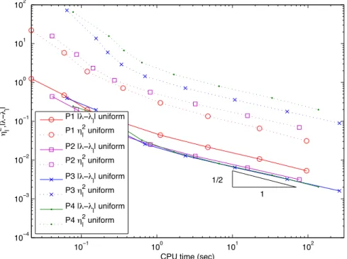
10ï1 100 101 102 103 10ï6 10ï5 10ï4 10ï3 10ï2 10ï1 100 101 102

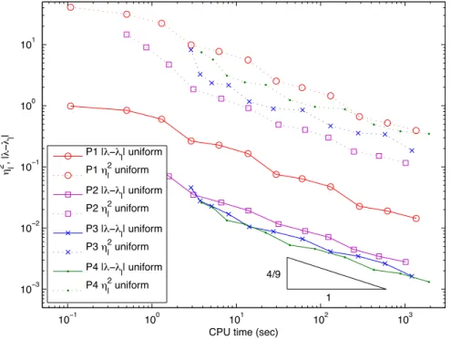
CPU time (sec) dl 2, | h ï hl | 1 2/3 1 1 1 4/3 1 4/9 P1 |hïh_l| adaptive P1 d l 2 _adaptive P2 |hïh_l| adaptive P2 d l 2 _adaptive P3 |hïh l| adaptive P3 d l 2 _adaptive P4 |hïh_l| adaptive P4 d l 2 _adaptive P4 |hïh l| uniform

Figure 1.2: State of the art quasi-optimal adaptive finite element method for eigenvalue computations on the 3D L-shaped domain: Eigenvalue errors as function of CPU time from Section 3.8 for various polynomial degrees.

to musicians aswolf tone. The problem is that an instrument specific tone that matches some eigenfrequency causes the instrument to sound like the howling of a wolf. Due to [54] this problem is caused by “the beating of two equal forces”. The first force is the string vibration while the second one is the body vibration. In this weakly damped coupled string-body system, the body withdraws energy from the string resulting in a lack of sound level. The musician tries to compensate that by putting more energy on the string which then leads to an increase of the sound level. The resulting up and down in the sound level is experienced as the howling of a wolf.

The third example of the occurrence of eigenvalue problems is the celebrated article of M. Kac (1966) [72]: “Can one hear the shape of a drum?” The question is whether two different shaped planar drums (of the same area) can have the same spectrum. The answer was published in C. Gordon D. Webb and S. Wolper (1992) [63]: “One cannot hear the shape of a drum”. The first eigenfunction for the two isospectral domains from [62] are depicted in Figure 1.1. An interesting empirical observation is that even the discrete eigenvalues coincide (up to round-off errors) when both domains are triangulated with the same number of similar shaped triangles.

1.2 State of the Art

The mathematical studies of eigenvalue problems dates back to the book of Helmholtz, Sensations of Tone (1863), which marks the foundation of acoustics.

The a priori error analysis of the finite element method of eigenvalue problems for partial differential equations (PDEs) started with the Laplace eigenvalue model problem [105]. The further development of the a priori error analysis [9, 42] led to the eigen-value chapter [10] with estimates for general compact operators and their application to general second-order elliptic operators. Further a priori error estimates for self-adjoint

operators can be found in [81, 98]. All those results assume that the global mesh-size is sufficiently small due to the non-linear nature of the eigenvalue problem. The article [100] investigates the convergence behaviour in the pre-asymptotic regime and [79] gives a priori error estimates with explicit constants and without the usual assumption that the mesh-size is sufficiently small.

The a posteriori error analysis of the finite element method started with [108] for symmetric second order elliptic eigenvalue problems based on a general non-linear anal-ysis. The duality-based analysis of [80] led to a posteriori error estimates for theL2 _and

energy errors but only for sufficiently smooth solutions. In [50] a residual a posteriori error estimator for non-smooth solutions is developed and it is proven that the volumet-ric part of the residual dominates the jumps for linear finite elements and the smallest eigenvalue. This result has been improved in [33] where it is shown that the volumetric part is not needed for all eigenvalues. Other a posteriori error estimator techniques have been employed for the eigenvalue problem as well. An averaging a posteriori error estimator has been presented in [89] and hierarchical a posteriori error estimators can be found in [65, 91, 92]. The results on symmetric eigenvalue problem have been applied to heterogeneous elastic structures in [109]. For the non-symmetric convection-diffusion eigenvalue problem a posteriori error estimators were presented in [69].

The asymptotic convergence analysis of the adaptive finite element method for sym-metric eigenvalue problems started with [60] based on a refinement procedure that con-siders both a standard a posteriori error estimator and the oscillations of eigenfunctions. Asymptotic convergence for a much simpler standard bulk marking strategy and the standard residual type a posteriori error estimator has been presented in [58]. Around the same time the article [33] proved asymptotic convergence for the pure edge-residual a posteriori error estimator.

Based on a coarsening procedure [44] presented the first results on asymptotic quasi-optimal convergenceof eigenvalue computations. For the adaptive finite element method [45] showed the first result without coarsening. The corresponding result for the Steklov eigenvalue problem can be found in [57]. However, all those results do unrealistically assume the exact knowledge of algebraic eigenpairs.

Assuming a saturation assumption, [91, 92] present combined adaptive finite element and linear algebra algorithms. Based on the dual-weighted residual method [96] pre-sented a balanced adaptive finite element and linear algebra algorithm for the non-symmetric convection-diffusion eigenvalue problem.

1.3 Overview and Main Results

This thesis aims at the numerical analysis of eigenvalue problems for the Laplace and the convection-diffusion operators. Fast algorithms (quasi-optimal for the Laplace op-erator and adaptive homotopy based for the convection-diffusion opop-erator) and sharp error bounds (via lower eigenvalue bounds for the Laplace operator and DWR-based a posteriori error estimators for the convection-diffusion operator) are presented. It is shown by various numerical experiments, or it is even proven for the Laplace operator,

that the adaptive finite element method decreases complexity of the eigenvalue com-putations and even improves the accuracy of the computed eigenvalues/eigenfunctions in comparison to uniform mesh-refinement. The following gives an overview of the five main parts of this thesis in Chapters 3–7 and presents the main results. The first three parts in Chapters 3–5 consider the symmetric Laplace eigenvalue problem while the last two parts in Chapters 6 and 7 concern a non-symmetric convection-diffusion eigenvalue problem.

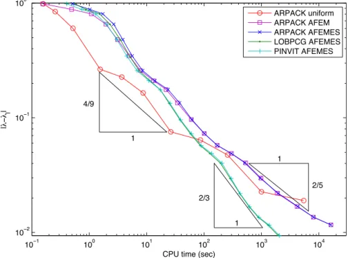
The motivation of the first part in Chapter 3 is that in practice the computational costs for the iterative algebraic eigenvalue solver dominate the overall computational costs. Hence, it is beneficial to stop the iterations of the algebraic eigenvalue solver at an early stage. In order to preserve the optimal order of convergence, the discretisation and the algebraic errors need to be balanced in the right way. Chapter 3 presents the first adaptive finite element eigenvalue solver (AFEMES) of overall asymptotic quasi-optimal complexity in terms of the CPU time as displayed in Figure 1.2. This is joint work with C. Carstensen and has been published in [34].

The main result is the asymptotic quasi-optimal computational complexity of the pro-posed AFEMES: Suppose that (λℓ, uℓ) is a discrete eigenpair to the continuous eigenpair

(λ, u). Let (Tℓ)ℓ be a sequence of nested regular triangulations and|||·|||denote the energy

norm. Suppose that the continuous eigenpair (λ, u) belongs to some approximation class

As, i.e., there exists somes >0 and some|u|As <∞ such that, for any numberN there

is an (unknown) optimal mesh TN with |TN| ≤ |T0|+N element domains and discrete

eigenpair (λN, uN) with

sup

N∈_N

N2s|||u−uN|||2+|λ−λN|=:|u|2As <∞.

Then the computational complexity of the AFEMES is quasi-optimal in the sense that

|||u−u˜ℓ|||2+|λ−λ˜ℓ| ≤ O(t−ℓ2s),

where tℓ denotes the computational costs in form of the CPU time. The point is that

this quasi-optimal complexity holds for any u ∈ As and all s > 0 despite the fact that

AFEMES does not require any parameter s. The analysis consists of three steps and does not need any inner node property, coarsening or saturation assumption. Since in the present analysis no oscillations occur, it is not necessary to add additional inner points to reduce some oscillations [60]. In [44] a coarsening of the mesh is needed in some steps to maintain optimality. The present analysis relies only on refinement of some mesh and does not need any coarsening. For hierarchical error estimators [91, 92] reliability is equivalent to the saturation assumption, namely a strict error reduction for uniform refined meshes. For the residual estimator used here the reliability is proven directly. First the asymptotic quasi-optimal convergence is shown for discrete eigenpairs without using the inner node property: Suppose that (λℓ, uℓ) is a discrete eigenpair to the

continuous eigenpair (λ, u) in some approximation classAsfor somes >0. Then (λℓ, uℓ)

Figure 1.3: Criss (left), criss-cross (middle) and union-jack (right) triangulations of the unit square in 2, 4, and 8 congruent triangles.

with

|||u−uℓ|||2+|λ−λℓ| ≤C|u|2_AsN_ℓ−2s.

In contrast to [45] the proofs are based on the eigenvalue formulation and not on a relation to its corresponding source problem. Hence, no additional oscillations arise from the corresponding source problem. The second step extends this result to the case of inexact algebraic eigenvalue solutions: Suppose (λ, u) withu∈ Asis an eigenpair and

(λℓ, uℓ) and (λℓ+1, uℓ+1) corresponding discrete eigenpairs on levels ℓ and ℓ+ 1. Let the

iterative approximations (˜λℓ,uℓ˜ ) on Tℓ and (˜λℓ+1,uℓ˜+1) on Tℓ+1 satisfy

|||uℓ+1−u˜ℓ+1|||2+|λℓ+1−˜λℓ+1| ≤ωηℓ2(˜λℓ,u˜ℓ),

|||uℓ−uℓ˜ |||2+|λℓ−λℓ˜ | ≤ωη_ℓ2(˜λℓ,uℓ˜ ),

for sufficiently small ω > 0. Then, the iterative solutions ˜λℓ and ˜uℓ converge quasi-optimal, up to some generic constantC >0,

|||u−u˜ℓ|||2+|λ−λ˜ℓ| ≤CNℓ−2s.

Finally, it is shown that the AFEMES is of linear runtime provided the linear algebra eigenvalue solver satisfies some convergence and complexity assumptions.

Numerical experiments show empirical quasi-optimal computational complexity of the AFEMES for some iterative algebraic eigenvalue solvers and higher-order finite element methods in 2 and 3 dimensions.

Thesecond part in Chapter 4 is motivated by the fact that the residual based a poste-riori error estimator involves some unknown constant and therefore the accuracy of the computed eigenvalues are much better than the termination criterion of the AFEMES suggests. Hence, sharp eigenvalue error bounds are needed in order to stop the compu-tation at an early stage when the desired accuracy is reached. One way to obtain sharp eigenvalue error bounds is to compute sharp upper and lower eigenvalue bounds. Upper bounds are easily obtained from the Rayleigh-Ritz principle while lower bounds may possibly be obtained by minimising the Rayleigh-quotient on some larger set of non-admissible functions. Chapter 4 presents lower bounds for eigenvalues of the Laplace

operator with the help of nonconforming finite element methods. This is joint work with C. Carstensen and has been accepted for publication [35].

The well-established Rayleigh-Ritz principle for the algebraic as well as for the con-tinuous eigenvalues of the Laplace operator immediately results inupper bounds of the eigenvalues by Rayleigh quotients

λ1 ≤R(v) :=|||v|||2/∥v∥2 for any v ∈H01\{0}. (1.1)

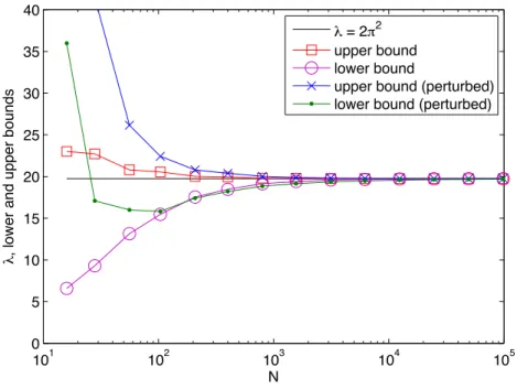
Since upper bounds are easily obtained by conforming discretisations via (1.1), the computation of lower bounds is of high interest and we solely mention the mile-stones [7, 55, 110] for asymptotic lower bounds in the sense that they provide guaranteed bounds under the assumption that the global mesh-size is sufficiently small. Unfortunately, the minimal mesh-size required to deduce some guaranteed lower eigenvalue bound is not quantified in the current literature – so nobody knows whether some mesh allows some guaranteed bound or not. Chapter 4 establishes guaranteed lower bounds even for very coarse triangulations like those of Figure 1.3 for the unit square Ω = (0,1)2 _{with only}

very few triangles. For the three meshes of Figure 1.3, clearly in the pre-asymptotic range of convergence, the first main result of Chapter 4 provides the guaranteed bounds

2.3371≤λ1 ≤32, 4.2594 ≤λ1 ≤24, and 6.6182≤λ1 ≤22.0397

for the first exact eigenvalue λ1 = 2π2 = 19.7392 despite the coarse discretisation with

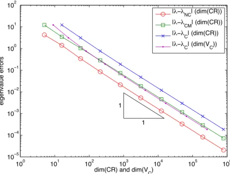
just 1, 4, or 8 degrees of freedom in a Crouzeix-Raviart nonconforming finite element discretisation (CR-NCFEM). To describe the main results of Chapter 3, letT be an arbi-trarily coarse shape-regular triangulation of the polygonal domain Ω into triangles with setE of edges and let CR1₀(T) denote the Crouzeix-Raviart nonconforming FEM spaces for the piecewise first-order polynomials. Suppose that (˜λCR,1,u˜CR,1) ∈ R ×CR10(T)

is some computed approximation of the smallest exact eigenvalue λ1 of the associated

algebraic eigenvalue problem with the stiffness matrix A, the (diagonal) mass matrix

B, and the algebraic residual r := Au˜CR,1 −λ˜CR,1Bu˜CR,1 for the algebraic

eigenvec-tor ˜uCR,1. Suppose that the first approximated discrete eigenvalue ˜λCR,1 is closer to

the first discrete eigenvalue λCR,1 than to the second discrete eigenvalue (which has to

be guaranteed by algebraic eigenvalue analysis) and that ∥r∥B−1 < λ˜_CR,1. Moreover, H := maxT∈T diam(T) denotes the maximal mesh-size and ICM denotes some

interpo-lation operator withICMu˜CR,1 ̸≡0. The first main result reads

˜

λCR,1− ∥r∥B−1

1 +κ2_(˜λ

CR,1− ∥r∥B−1)H2

≤λ≤R(ICMu˜CR,1).

The explicit constant κ reads κ2 _{:= (1/8 +j}−2

1,1) ≤ 0.1932 for the first positive root

j1,1 = 3.8317059702 of the Bessel function of the first kind. Note that the nonconforming

eigenvalue for the first two meshes of Figure 1.3 reads λCR₀ = 24 and is larger than the solution λ = 2π2_{. This novel observation shows that the nonconforming eigenvalue by}

to the lower bound given in Chapter 4. The asymptotic a posteriori error control of [7] does not provide those error bounds.

The second main result guarantees efficiency in the sense that the difference of the upper and lower bound is bounded by the error for the large class of graded meshes.

The lower bound is generalised to higher eigenvalues under some explicit given mesh-size restriction plus the aforementioned separation condition. Together with a conform-ing approximation for an upper bound, the bounds for the higher eigenvalues are also efficient.

The efficiency for graded meshes motivates the development of an adaptive algorithm that balances the finite element error and the global mesh size H in order to reduce the difference of the upper and lower eigenvalue bounds. Numerical experiments show convergence of the proposed AFEM and compare conforming and nonconforming dis-cretisations empirically.

For the third part in Chapter 5 note that the quasi-optimal algorithm of Chapter 3 is based on a contraction property of the sum of the errors of the eigenfunctions in energy norm plus the residual a posteriori error estimators and this does not imply contraction of the error itself but only proves that either the error or the a posteriori error estimator or both decrease during the adaptive finite element loop. Therefore the question arises whether there exists a refinement strategy that yields contraction of the error on its own. Chapter 5 presents an adaptive finite element method that yields such an asymptotic error reduction. This is joint work with C. Carstensen, V. Mehrmann and A. Miedlar and is submitted for publication [38].

The error reduction (also called saturation) property for the linear second order bound-ary value problem is reasonably justified in [1, 13, 49, 53, 108]. For the eigenvalue problem, the mathematical justification of the adhoc saturation assumption in [91, 92] is widely open even in the asymptotic range for extreme small mesh-sizes. Chapter 5 appears to be the first contribution to the mathematical foundations of the saturation property

ˆ

λℓ−λ≤ϱ(λℓ−λ) + HOT,

for the discrete eigenvalueλℓto some simple eigenvalueλ, some higher-order and/or

fine-grid solutionλℓ , and some 0≤ϱ <1. In [91, 92], the contribution HOT is neglected while

this chapter computes the explicit contribution HOT := ˆλ3

ℓHℓ4 and therefore justifies

that this term can be neglected for very fine meshes. It is true that [33] shows that oscillations can be neglected under certain particular assumptions on the meshes, but the same global arguments do not apply in the present situation where the analysis is based on local estimates.

Chapter 5 presents an adaptive finite element method with asymptotic saturation of asingle sequence of eigensolutions (λℓ, uℓ)ℓ∈N0 in the following sense. There exists some

Hℓ it holds that |λ−λℓ+1|+|||u−uℓ+1|||2 ≤ϱ  |λ−λℓ|+|||u−uℓ|||2  + 2λ3_ℓ+1H_ℓ4.

The adaptive algorithm utilises a patch-oriented refinement process based on the red-green-bluerefinement without the interior node property and there is no need to compute any higher-order or fine-grid solutions. Note that the higher-order term 2λ3

ℓ+1Hℓ4 is

explicit even with the multiplicative constant 2 in front of it.

Numerical examples verify the (asymptotic) reliability and efficiency of the hierar-chical a posteriori error estimator and therefore confirm the (asymptotic) saturation property. For the first eigenvalue the mesh-size restrictions on H0 are empirically not

visible, but are certainly more severe for larger eigenvalues with much more oscillating eigenfunctions.

Thefourth part considers the non-symmetric convection-diffusion eigenvalue problem. Since the residual based a posteriori error estimator involves some unknown constant that depends on the convection-coefficient, other techniques that lead to sharp error bounds are of high interest. Chapter 6 presents (empirically) sharp a posteriori error estimators for the convection-diffusion eigenvalue problem based on the dual-weighted residual (DWR) method. This is joint work with C. Carstensen and will be published in [59].

While the numerical approximation of eigenvalues of symmetric second-order elliptic PDEs with real eigenpairs is relatively well understood, much less is known about non-symmetric problems with possibly complex eigenvalues. A posteriori error estimators for some non-symmetric eigenvalue problems can be found in [43, 69, 70]. It is the aim of Chapter 6 to review the results of Heuveline and Rannacher in a direct approach rather than in the non-linear setting of the DWR paradigm after [12, 14, 69]. These results are also applicable to the averaging techniques as for the symmetric eigenvalue problem in [89]. The first two residual and averaging based a posteriori error estimators are based on the residual estimate for the eigenvalue error with dual energy norm|||·|||∗, primal and dual residuals Resℓ, Res∗ℓ, and some generic constant C > 0,

|λ−λℓ| ≤C  |||Resℓ|||2∗+|||Res ∗ ℓ||| 2 ∗  .

Therefore, the dual norms of the primal and dual residuals can be bounded separately. Numerical experiments indicate that the efficiency indices for the residual-type a pos-teriori error estimators depend strongly on the convection coefficient β. Therefore, this chapter investigates the dual-weighted residual paradigm from Becker and Rannacher [12, 14, 15]. The DWR based a posteriori error estimators are derived from the asymp-totic sharp estimate for simple (non-degenerate) eigenvalues λ with primal and dual eigenfunctionsu, u∗ ∈H1

0(Ω;C),

|λ−λℓ| ≤C|Resℓ(u∗−u∗ℓ) + Res

∗

ℓ(u−uℓ)|,

dual-Figure 1.4: Schematic view of three homotopy-based Algorithms.

weighted residual a posteriori error estimators avoid any additional inequality, such as approximation properties with unknown constants. Thus, they are robust with respect to strong convection which is also confirmed by the numerical examples in Section 6.5. One question that arises from the computation of Resℓ(u∗ −u∗ℓ) or Res

∗

ℓ(u−uℓ) is the

calculation of the unknown primal and dual errorsu−uℓandu∗−u∗_ℓ. The rather heuristic approach of [12] states that it is numerically reliable and efficient to approximate these quantities which occur only in the weights. The idea is that one does not need to approximate the weights with higher accuracy than the size of the residual terms. In practice the unknown primal and dual solutions u, u∗ are replaced by solutions of a higher-order method or by some higher-order interpolation. Benchmark experiments provide numerical evidence that the DWR methodology in combination with the L2

interpolation scheme of [111] is empirical reliable and efficient for unstructured triangular meshes while [69] is restricted to structured meshes because of the approximation of the weights by second-order difference quotients. In addition, two new dual-weighted a posteriori error estimators are presented. The first new estimator is based on the Raviart-Thomas mixed finite element method (MFEM) of first-order and the second one on averaging techniques. Hence, they are named by dual-weighted mixed (DWM) and dual-weighted averaging (DWA) a posteriori error estimators.

The fifth part contributes to the fact that the eigenvalues for the non-symmetric convection-diffusion eigenvalue problem may be ill-conditioned and the (symmetric) Rayleigh-Ritz principle does not hold. Therefore, it is harder to guarantee convergence of some iterative algebraic eigenvalue solver towards some specific eigenvalue. The idea is now to first compute the eigenvalues for the simpler symmetric eigenvalue problem where the eigenvalues converge safely and then bring in the non-symmetric part via a homotopy method. Chapter 7 presents three versions of adaptive homotopy algorithms for the convection-diffusion eigenvalue problem. This is joint work with C. Carstensen, V. Mehrmann and A. Miedlar and has been published in [37].

The difficulty with non-selfadjoint PDE eigenvalue problems is multifold, eigenval-ues may be complex, or may have different algebraic and geometric multiplicity. The latter property is a particular difficulty because this property is destroyed in the finite dimensional approximation. The computed eigenvalues and eigenfunctions may have

large errors due to the ill-conditioning of the problem although the approximation error is small. Even when the discretisation retains the multiplicities of the eigenvalues, the algebraic eigensolvers have difficulties with the ill-conditioning of multiple eigenvalues.

Chapter 7 studies the restricted class of convection-diffusion eigenvalue problems and simple eigenvalues, where for the pure diffusion problem the discussed adaptive methods work nicely. To design a robust adaptive algorithm for the convection-diffusion problem a homotopy method is applied. Homotopy methods are well established for non-symmetric matrix eigenvalue problems [84, 85, 86, 88]. Here, the homotopy approach is used not only on the matrix level but on the level of the differential operator as well. The continuation method uses a ’time’-stepping procedure with nodes t0 = 0 < t1 < . . . <

tN = 1 to compute the eigenvalues and eigenvectors of

−∆u+tiβ· ∇u=λu in Ω.

The final homotopy value 1 results in the desired problem

−∆u+β· ∇u=λu in Ω.

The combination of the adaptive homotopy with mesh adaptivity and iterative matrix eigenvalue solvers involves three different types of errors: the discretisation error η

that arises when the infinite dimensional variational problems is considered in a finite dimensional subspace [69] and Chapter 6, the homotopy errorν that arises because the diffusion problem is slowly transferred to the convection-diffusion problem [22] and the approximation errorµthat arises from the iterative matrix eigensolver in finite precision arithmetic [11, 68, 94, 104]. To develop adaptive algorithms that are adaptive with respect to all three types of errors, three different algorithms are proposed as depicted in Figure 1.4. The first algorithm balances the homotopy, the discretisation and the approximation errors with respect to a fixed step-size in the homotopy. The second algorithm combines the adaptive step-size control for the homotopy with an adaptation in space that ensures an error below a fixed tolerance. The outcome leads to the third algorithm which allows the complete adaptivity in space, homotopy step-size as well as the iterative algebraic eigenvalue solver. The overall eigenvalue error is shown to be bounded by the a posteriori eigenvalue error bound

|λ(1)−λ˜ℓ(t)| ≤C



ν(˜λℓ(t),u˜ℓ(t),u˜∗ℓ(t)) +η2(˜λℓ(t),u˜ℓ(t),u˜∗ℓ(t)) +µ2(˜λℓ(t),u˜ℓ(t),u˜∗ℓ(t))



,

in terms of the homotopy a posteriori error estimator ν(˜λℓ(t),u˜ℓ(t),u˜∗ℓ(t)), the

discreti-sation a posteriori error estimator η2_(λ

ℓ(t), uℓ(t), u∗ℓ(t)), the algebraic a posteriori error

estimator µ2(˜λℓ(t),uℓ˜ (t),u˜∗_ℓ(t)), and some generic constant C > 0.

1.4 Outlook and Open Questions

For an outlook and open questions note that, despite the guaranteed lower eigenvalue bounds of Chapter 4, this work restricts to simple eigenvalues. For the symmetric

prob-lem a convergence result of the adaptive finite eprob-lement method for multiple or clustered eigenvalues has been proven in [33]. This convergence result is based on a refinement strategy that refines the mesh accordingly to the sum of the a posteriori error estima-tors of all the discrete eigenfunctions to some multiple eigenvalue. The open question is whether this leads to optimal convergence of one particular eigenfunction. The fact that different eigenfunctions of the eigenspace to some multiple eigenvalue may have different regularity rises the question whether for larger eigenspaces adaptive mesh-refinement is better than just uniform refinement. In the case of non-symmetric eigenvalue problems the possible blow up of the condition number of clustered/multiple eigenvalues makes efficient error control impossible. Besides the question of multiple or clustered eigen-values there is a number of open questions for simple eigeneigen-values that result from this thesis as well. Open questions include the quasi-optimal convergence of the adaptive nonconforming finite element method for the eigenvalue problem as it is shown for the conforming finite elements in Chapter 3. Nonconforming methods, that provide lower eigenvalue bounds for the Laplace operator as shown in Chapter 4, play an important role in the stabilisation of numerical schemes such as the locking-free Kouhia-Stenberg finite element for linear elasticity. Does the Kouhia-Stenberg finite element provide lower eigenvalue bounds for linear elasticity? The techniques of Chapter 4 inspired [32] for lower eigenvalue bounds for fourth-order problems such as the Kirchhoff-Plate. Other possible future research activities may lead to lower eigenvalue bounds in the context of the stability analysis of time-evolution problems. Concerning the non-symmetric eigenvalue problems, future work will extend the homotopy algorithms of Chapter 7 to more complex eigenvalue problems such as the quadratic eigenvalue problems arising in dissipative acoustics [16]. The homotopy method enables the computation of some non-zero complex eigenvalues with certain features of interest of the indefinite quadratic eigenvalue problem without the need of full matrix decompositions.

The summary of the functional analysis background in Section 2.1 is derived from [27, 52]. The presentation of the finite elements in Section 2.2 is based on [23, 27]. The a priori results for the model PDE eigenvalue problems in Section 2.3 and Section 2.4 have been taken from [10, 20, 105]. Adaptive mesh-refinement algorithms are described in Section 2.5 following [1, 8, 108].

Throughout this thesis, the notation x _. y abbreviates the inequality x ≤ Cy and

x ≈ y the inequalities Dy ≤ x ≤ Cy with constants C > 0 and D > 0 which do not depend on the mesh-size.

2.1 Functional Analysis Background

Let Ω be a connected open subset of _Rn _{that is Lebesgue-measurable. The Lebesgue}

integral over Ω for real valued functionsf that are Lebesgue measurable is ´_Ωf dx. The Lebesgue spaces are defined for 1≤p <∞,

Lp(Ω) :={f :∥f∥Lp_(Ω) <∞}

with the Lebesgue norms

∥f∥p_Lp_(Ω) :=

ˆ Ω

|f|p_dx.

The norm forp=∞ is defined as

∥f∥L∞_(Ω) := ess sup{|f(x)|:x∈Ω}.

The Lebesgue spaces are Banach spaces. Moreover, in this thesis p= 2 and L2_{(Ω) is a}

Hilbert space withL2-scalar product

ˆ Ω

f g dx for any f, g ∈L2(Ω).

The following inequalities are frequently used in this thesis.

Lemma 2.1.1(Minkowski’s inequality). For 1≤p≤ ∞ andf, g ∈Lp(Ω), it holds that

∥f+g∥Lp_(Ω) ≤ ∥f∥_Lp_(Ω)+∥g∥_Lp_(Ω).

f ∈Lp(Ω) and g ∈Lq(Ω), it holds that f g∈L1(Ω) and

∥f g∥L1_(Ω) ≤ ∥f∥_Lp_(Ω)∥g∥_Lq_(Ω).

In the special casep=q= 2 this inequality is called Cauchy-Schwarz inequality.

Lemma 2.1.3 (Cauchy-Schwarz inequality). For f, g∈L2(Ω) it holds thatf g ∈L1(Ω) and

ˆ Ω

f g dx≤ ∥f∥L2_(Ω)∥g∥_L2_(Ω).

LetCm_{(Ω), m ∈}

N, denote the space of m-times continuously differentiable functions

and the subset Cm

0 (Ω) those functions with compact support.

The function f ∈ L2(Ω) has a weak derivative (in L2(Ω)) if there exists a function

g =∂α_{u such that} ˆ Ω gϕ dx= (−1)|α| ˆ Ω f ∂αϕ dx for all ϕ∈C₀∞(Ω).

Letm∈_N and f ∈L2_{(Ω) such that all weak derivatives∂}α_{f with |α| ≤m exist. Then}

∥f∥2 Hm_(Ω) :=  |α|≤m ∥∂αf∥2 L2_(Ω) is a norm and |f|2 Hm_(Ω) :=  |α|=m ∥∂αf∥2 L2_(Ω)

a semi-norm. The Sobolev spaces to L2_{(Ω) are defined as}

Hm(Ω) :={f ∈L2(Ω) :∥f∥Hm_(Ω) <∞}.

Sobolev spaces Hm_{(Ω) are Hilbert spaces. For domains Ω with Lipschitz boundary, the}

Sobolev spaces have boundary values in the sense of traces.

Theorem 2.1.4 (Trace theorem). Suppose that Ω has a Lipschitz boundary ∂Ω, then there exists a constantC > 0 such that

∥f∥L2_(∂Ω) ≤C∥f∥1_L/22_(Ω)∥f∥

1/2

H1_(Ω) for all f ∈H1(Ω).

The subset of H1_{(Ω) with zero trace on the boundary∂Ω defines}

H₀1(Ω) :={f ∈H1(Ω) :f|∂Ω = 0 inL2(∂Ω)}.

For the spaceH1

0(Ω), the semi-norm |.|H1_(Ω) is actually a norm.

The domain Ω ⊆ _Rn _{is star-shaped with respect to a ball B if the convex hull of}

Lemma 2.1.5(Poincaré’s inequality). Suppose that Ωis the finite union of star-shaped domains with respect to a ball. Then there exists a constant CP <∞ such that

∥f∥L2_(Ω)≤C_P|f|_H1_(Ω) for all f ∈H₀1(Ω).

Letffl_Ωf dx denote the integral mean value _|Ω1_|´_Ωf dx.

Lemma 2.1.6 (Friedrichs’ inequality). Suppose thatΩis the finite union of star-shaped domains with respect to a ball. Then there exists a constant CF <∞ such that

     f− Ω f dx     _L2_(Ω) ≤CF|f|H1_(Ω) for all f ∈H1(Ω).

Suppose that Ω is a bounded Lipschitz domain, then the Gauss-divergence theorem and the integration by parts formula hold.

Theorem 2.1.7 (Gauss-divergence theorem). Suppose that f ∈ C1_{(Ω)∩C(Ω), then it}

holds that ˆ Ω div(f)dx = ˆ ∂Ω f ν ds.

Theorem 2.1.8(Integration by parts formula). Suppose that f, g∈C1(Ω)∩C(Ω), then it holds that ˆ Ω  ∂f ∂xj g+f ∂g ∂xj  dx= ˆ ∂Ω f gνjds. for 1≤j ≤n.

2.2 Finite Elements

According to the definition due to Ciarlet, a finite element is a triple (T, PT, NT) [27] where

1. T ⊆ _Rn _{is a bounded closed set with non-empty interior and piecewise smooth}

boundary,

2. PT is a finite-dimensional space of functions onT and

3. NT ={N1, . . . , Nm}is a basis for the dual space PT′.

The finite element function space PT is the space of shape functions and NT the set of

nodal variables.

The nodal basis {ϕ1, . . . , ϕm} of PT for some finite element (T, PT, NT) is the basis

that is dual to NT, that is Ni(ϕj) = δi,j for Kronecker’s δi,j = 0 for i ̸= j and δi,j = 1

Figure 2.1:Pk, k = 1,2,3,4, finite element.

2.2.1 Conforming Finite Element

As an example of aH1-conforming finite element consider the triangular Lagrange finite elements. Let PT be the space of polynomials of degree ≤ k and NT be the shape

functions that consist of the point evaluation in the barycentric coordinates as depicted in Figure 2.1 for k= 1,2,3,4.

As a consequence of the Bramble-Hilbert lemma [27, (4.3.8)], the nodal interpolation operatorI satisfies the following approximation property.

Lemma 2.2.1 ([27, (4.4.4)]). For all v ∈ H2(T) there exists a constant C < ∞ such that for the diameter diam(T) := sup_x,y∈T|x−y|

|v− Iv|_H1_(T)≤Cdiam(T)|v|_H2_(T).

For the linear triangular Lagrange finite element the constant C is explicitly bounded by C(α) :=     1/4 + 2/j2 1,1 1− |cos(α)|,

for the maximal angle 0 < α < π of the triangle T and the first positive root of the Bessel functionJ1 [39].

2.2.2 Nonconforming Finite Element

The H1_{-nonconforming Crouzeix-Raviart finite element consists of the affine functions}

PT and the shape functionsNT that consist of the point evaluation in the midpoints of

the three edges as depicted in Figure 2.2.

The nonconforming interpolantINCspecifies the values for the edge degrees of freedom

as INCv(mid(E)) := 1 |E| ˆ E

v ds for all edges E of T.

The following approximation estimate with explicit constant holds [39], cf. Theo-rem 4.2.1, ∥v− INCv∥L2_(T) ≤  diam(T)2_{/8 + diam(T)}2_/j2 1,1 |v− INCv|H1_(T).

2.3 The Symmetric Model Eigenvalue Problem

As a simple model problem for a symmetric, elliptic eigenvalue problem consider the following eigenvalue problem of the Laplace operator: Seek a non-trivial eigenpair (λ, u)∈_R× {H1_(Ω;

R)∩Hloc2 (Ω;R)} such that

−∆u=λu in Ω and u= 0 on∂Ω (2.1)

in a bounded Lipschitz domain Ω⊂ _Rn_{, n = 2,3. It is well known, that problem (2.1)}

has countably many solutions with positive eigenvalues that can be ordered increasingly 0< λ1 ≤λ2 ≤λ3 ≤. . .

and there exist some orthonormal basis (u1, u2, u3, ...) of corresponding eigenvectors.

The weak problem seeks for a non-trivial eigenpair (λ, u)∈_R× {V :=H1

0(Ω;R)}with

b(u, u) = 1 and

a(u, v) =λb(u, v) for all v ∈V.

The bilinear forms a(·,·) and b(·,·) are defined by

a(u, v) := ˆ Ω ∇u· ∇v dx and b(u, v) := ˆ Ω uv dx

and induce the norms|||.|||:=|.|H1_(Ω;

R) onV and ∥.∥:=∥.∥L2(Ω;R) on L

2_(Ω; R).

2.3.1 Conforming Discrete Eigenvalue Problem

The conforming finite element space of orderk ∈_N for the shape-regular triangulation of the polygonal domain Ω into triangles T is defined by

Pk(T) :=



v ∈L2(Ω;_R) :∀T ∈ T, v|T is polynomial of degree≤k



.

Let VC :=Pk(T)∩H01(Ω;R) denote the finite-dimensional subspace of fixed order k >

0. The corresponding discrete eigenvalue problem reads: Seek a non-trivial eigenpair (λC, uC)∈R×VC with b(uC, uC) = 1 and

a(uC, vC) =λCb(uC, vC) for all vC ∈VC.

Lemma 2.3.1. LetVC be the conforming finite element space of orderk andλC a simple

eigenvalue. For sufficiently small global mesh-size Hℓ it holds that

|λ−λC|+|||u−uC|||2 .H

max(s,2k)

ℓ λ

k+1_,

where s >0 depends on the regularity of the solution.

For multiple eigenvalues similar a priori estimates hold [10]. 2.3.2 Nonconforming Discrete Eigenvalue Problem

Let T be an arbitrarily shape-regular triangulation of the polygonal domain Ω into triangles with setE of edges and let

CR1₀(T) :={v ∈P1(T)|v is continuous at mid(E) andv = 0 at mid(E(∂Ω))}

denote the Crouzeix-Raviart nonconforming FEM spaces for the piecewise first-order polynomialsP1(T). For all interior edgesE ∈ E(Ω), the edge-oriented basis functionψE

is defined by

ψE(mid(E)) = 1 and ψE(mid(F)) = 0 for all F ∈ E\E.

Then CR1₀(T) = span{ψE|E ∈ E(Ω)} * V and the nonconforming discrete eigenvalue

problem reads: Seek an eigenpair (λCR, uCR)∈R×CR01(T) with b(uCR, uCR) = 1 and

aNC(uCR, vCR) =λCRb(uCR, vCR) for all vCR∈CR10(T).

The nonconforming bilinear formaNC,

aNC(uCR, vCR) :=  T∈T ˆ T ∇uCR· ∇vCRdx for all uCR, vCR∈CR10(T),

induces the mesh-dependent norm |||.|||NC := aNC(·,·)1/2. For the nonconforming finite

element solutions the following a priori error estimates [7] holds.

Lemma 2.3.2. For the Crouzeix-Raviart nonconforming finite element space, simple eigenvalues and sufficiently small global mesh-size Hℓ, it holds that

|λ−λCR|+|||u−uCR|||2NC .H

max(s,2)

ℓ ,

2.4 The Non-Symmetric Model Eigenvalue Problem

The convection-diffusion model eigenvalue problem reads: Seek an eigenpair (λ, u) ∈

C× {H01(Ω;C)∩Hloc2 (Ω;C)}with

−∆u+β· ∇u=λu in Ω.

The given data β ∈ H(div,Ω;_R2_{) is supposed to be divergence free in the bounded}

Lipschitz domain Ω⊆_R2_{, i.e.,} ´

Ωvdivβ dx= 0 for allv ∈V :=H 1

0(Ω;C).

The weak problem considers the two complex Hilbert spaces V with energy norm

|||·||| =|·|H1_(Ω;

C) (which is a norm on V) and W := L

2_(Ω;

C) with norm ∥·∥L2_(Ω;

C). The

weak form reads: Seek an eigenpair (λ, u)∈_C×V with ∥u∥= 1 such that

a(u, v) =λb(u, v) for all v ∈V. (2.2) The bilinear form a(·,·) is elliptic and continuous in V and the bilinear form b(·,·) is continuous, symmetric and positive definite, and hence induces a norm ∥·∥ := b(·,·)1/2

onW. For the above model problem, ∥·∥=∥·∥L2_(Ω;

C) and the bilinear forms (where (·)

denotes complex conjugation) read

a(u, v) = ˆ Ω (∇u· ∇v+ (β· ∇u)v) dx and b(u, v) = ˆ Ω uv dx.

Sinceβ is assumed to be divergence free, an integration by parts yields

ˆ Ω (β· ∇v)v dx=− ˆ Ω (β· ∇v)v dx.

Hence, for all v ∈V, it holds that

|||v|||2 _{= Rea(v, v).}

Thus, the ellipticity constant (which is one) of the bilinear forma(·,·) is independent of the convection-coefficientβ.

The analysis of the non-symmetric eigenvalue problem requires the dual eigenvalue problem: Seek a (dual) eigenpair (λ∗, u∗)∈_C×V with ∥u∗∥= 1 such that

a(v, u∗) = λ∗_{b(v, u}∗_{) for all v ∈V.}

Since the embedding of V in W is continuous and compact, the spectral theory for compact operators [10, 73] is applicable. The Riesz-Schauder theorem shows that the primal and dual spectra consist of finite or countably many eigenvalues with no finite accumulation point. In particular, the algebraic multiplicities are finite.

Given any conforming finite-dimensional subspaceVℓ ⊂V, the discrete problems read:

Seek primal and dual (discrete) eigenpairs (λℓ, uℓ) and (λ∗ℓ, u

∗

Figure 2.3: Red, green and blue refinement. The new reference edge is marked through a second line in parallel opposite the new vertices new1, new2 or new3.

such that

a(uℓ, vℓ) =λℓb(uℓ, vℓ) for all vℓ ∈Vℓ; a(vℓ, u∗ℓ) =λ

∗

ℓb(vℓ, u∗ℓ) for all vℓ ∈Vℓ.

The primal and dual eigenvalues λj and λ∗j as well as the primal and dual discrete

eigenvaluesλℓ,j and λ∗ℓ,j are connected by

λj =λ∗j for j = 1,2,3, . . . and λℓ,j =λ∗ℓ,j for all j = 1, . . . ,dim(Vℓ).

The abstract a priori theory yields the following upper bounds in terms of the maximal mesh-size Hℓ for the linear conforming finite element approximations,

|λ−λℓ|_.Hs1+s2 ℓ , |||u−uℓ|||.H s1 ℓ , |||u ∗₋ u∗_ℓ|||_.Hs2 ℓ ,

where 0 < s1 ≤ 1 and 0 < s2 ≤ 1 depend on the regularity of the primal and dual

eigenfunctions [10, Chapter 10.3].

2.5 Adaptive Mesh-Refinement Algorithms

Let Tℓ be a sequence of regular triangulations in the sense of Ciarlet of the bounded

Lipschitz domain Ω into at least two triangles such that all T ∈ Tℓ are closed triangles

with positive area|T|and two distinct intersecting triangles T1, T2 ∈ Tℓ share either one

common edge or one common node. LetEℓdenote the set of all edges of the triangulation

2.5.1 Closure Algorithm

Given a triangulation Tℓ on the level ℓ, let E(T) denote the reference edge for a given

triangle T. To preserve the quality of the mesh, the closure algorithm computes the smallest subset M_ℓ of E_ℓ which includes all marked edges of the subset M_ℓ ⊆ E_ℓ of

selected edges for refinement such that



E(T) :T ∈ Tℓ with Eℓ(T)∩M_ℓ ̸=∅ 

⊆Mℓ.

In other words, once an edgeE of an element T is marked for refinement, the reference edge E(T) of T is marked as well.

An important result for the proof of optimality of the mesh-refinement is that the closure algorithm marks only a constant number of additional edges over all levels.

Proposition 2.5.1 (Boundedness of closure, [19, 103]). Let Tℓ+1 be a refinement of Tℓ,

obtained using one of the refinement algorithms below and the closure algorithm. Suppose

T0 is the initial coarse triangulation. Then it holds that

|TL| − |T0|.

L−1 

ℓ=0

|Mℓ|,

where |Tℓ| denotes the cardinality of all triangles in Tℓ.

2.5.2 Red-Green-Blue Refinement

Given a triangulation Tℓ on the level ℓ, let E(T) denote the reference edge for a given

triangle T ∈ Tℓ. Note that the reference edge E(T) will be the same edge of T in all

triangulations Tℓ which include T. However, once T inTℓ is refined, the reference edges

will be specified for the different sub-triangles as indicated in Figure 2.3.

The red-green-blue mesh-refinement algorithm consists of the following five different refinements. Elements with no marked edge are not refined, elements with one marked edge are refinedgreen, elements with two marked edges are refinedblue-left orblue-right, and elements with three marked edges are refined red as depicted in Figure 2.3.

2.5.3 Newest-Vertex Bisection

Thenewest-vertex algorithm consists of successive bisections of triangles until no hanging node remains. Thereby, always the edge opposite to the newest vertex is bisected. Hence, in the notion of reference edges, E(T) is always opposite to the newest vertex of each triangleT ∈ Tℓ.

Therefore, after the closure algorithm is applied, one of the following refinement rules is applicable, namelyno refinement, green refinement, blue left or blue right refinement andbisec3 refinement as depicted in Figure 2.4. Note that the case of three marked edges is refined differently for thenewest-vertex refinement and the red-green-blue algorithm.

A corresponding newest-vertex bisection refinement algorithm for n= 3 based on the concept of reference edges can be found in [8].

Figure 2.4:Bisec3,greenandbluerefinement. The new reference edge is marked through a second line in parallel opposite the new vertices new1, new2 or new3.

The newest-vertex bisection algorithm allows for an overlay estimate that is one of the key arguments in the proof of quasi-optimality. For two arbitrary refinements Tℓ

andTm of the initial triangulationT0 define the overlayTℓ⊕ Tm as the smallest common

refinement such that all triangles ofTℓ and Tm are either contained or further refined in

Tℓ⊕ Tm.

Proposition 2.5.2 (Overlay, [41, 102]). The smallest common refinement of Tm and

Tℓ, Tm⊕ Tℓ, satisfies

Asymptotic Quasi-Optimal Computational Complexity

This chapter presents a combined adaptive finite element method with an iterative alge-braic eigenvalue solver for a symmetric eigenvalue problem of asymptotic quasi-optimal computational complexity. The analysis is based on a direct approach for eigenvalue problems and allows the use of higher-order conforming finite element spaces with fixed polynomial degree. The asymptotic quasi-optimal adaptive finite element eigenvalue solver (AFEMES) involves a proper termination criterion for the algebraic eigenvalue solver and does not need any coarsening. Numerical evidence illustrates the asymptotic quasi-optimal computational complexity in 2 and 3 dimensions.

This chapter is joint work with C. Carstensen and has been published in [34].

3.1 Introduction

The eigenvalue problems for symmetric second-order elliptic boundary value problems can be discretised with some adaptive finite element method (AFEM). In practice, the resulting finite-dimensional generalised eigenvalue problems are solved iteratively. Thus, the computation involves the discretisation error of some AFEM as well as the error left from the termination of some iterative algebraic eigenvalue solver. This chapter presents the first adaptive finite element eigenvalue solver (AFEMES) of overall asymptotic quasi-optimal complexity, i.e., for sufficiently small mesh-sizes the error is quasi-optimal up to a generic multiplicative constant. AFEMES is shown in the pseudocode below.

The algorithm computes one fixed simple eigenvalue. The adaptive mesh refinement via subroutines Mark and Refine is well-established in the finite element community [19, 41, 48, 102] whileLAESrepresents any state-of-the-art iterative eigenvalue solver well-established in the numerical linear algebra community that satisfies the convergence and