Aberystwyth University
Adaptive fuzzy interpolation
Yang, Longzhi; Shen, Qiang
Published in:
IEEE Transactions on Fuzzy Systems DOI:
10.1109/TFUZZ.2011.2161584
Publication date: 2011
Citation for published version (APA):
Yang, L., & Shen, Q. (2011). Adaptive fuzzy interpolation. IEEE Transactions on Fuzzy Systems, 19(6), 1107-1126. https://doi.org/10.1109/TFUZZ.2011.2161584
General rights
Copyright and moral rights for the publications made accessible in the Aberystwyth Research Portal (the Institutional Repository) are retained by the authors and/or other copyright owners and it is a condition of accessing publications that users recognise and abide by the legal requirements associated with these rights.
• Users may download and print one copy of any publication from the Aberystwyth Research Portal for the purpose of private study or research.
• You may not further distribute the material or use it for any profit-making activity or commercial gain • You may freely distribute the URL identifying the publication in the Aberystwyth Research Portal
Take down policy
If you believe that this document breaches copyright please contact us providing details, and we will remove access to the work immediately and investigate your claim.
tel: +44 1970 62 2400 email: [email protected]
Adaptive Fuzzy Interpolation
Longzhi Yang, Student Member, IEEE, and Qiang Shen
Abstract—Fuzzy interpolative reasoning strengthens the power
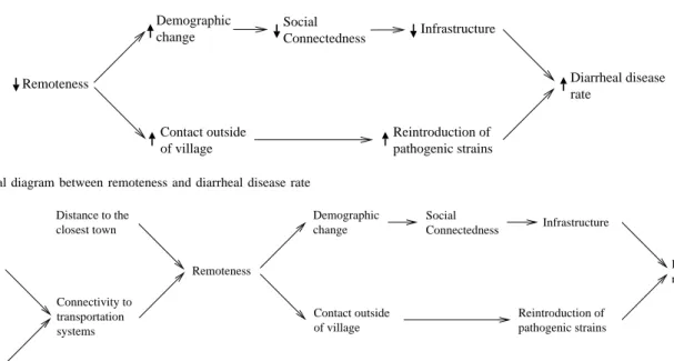
of fuzzy inference by enhancing the robustness of fuzzy systems and reducing systems complexity. However, after a series of interpolations, it is possible that multiple object values for a common variable are inferred, leading to inconsistency in inter-polated results. Such inconsistencies may result from defective interpolated rules or incorrect interpolative transformations. This paper presents a novel approach for identification and correc-tion of defective rules in interpolative transformacorrec-tions, thereby removing the inconsistencies. In particular, an assumption-based truth maintenance system is used to record dependencies between interpolations, and the underlying technique that the classi-cal general diagnostic engine employs for fault loclassi-calization is adapted to isolate possible faulty interpolated rules and their associated interpolative transformations. From this, an algorithm is introduced to allow for the modification of the original linear interpolation to become first-order piecewise linear. The approach is applied to a realistic problem, which predicates the diarrheal disease rates in remote villages, to demonstrate the potential of this work.
Index Terms—Fuzzy rule interpolation, assumption-based
truth maintenance, general diagnostic engine.
I. INTRODUCTION
Fuzzy rule interpolation significantly improves the robust-ness of fuzzy reasoning. It provides a way to reduce the complexity of fuzzy systems by omitting those rules which can be approximated by their neighboring ones. Also, it improves the applicability of fuzzy systems by allowing a certain conclusion to be generated even if the existing rule base does not cover a given observation. A number of important interpolating approaches have been presented in the literature, including [9], [12], [13], [31], [36], [37], [38], [42], [43], [44], [45], [54], [56], [60], [63], [64].
Common to these fuzzy interpolation techniques is the fact that interpolation is carried out in a linear manner. However, this is not always feasible when dealing with realistic problems and hence, may lead to inconsistencies in inferred rules and reasoning results after a sequence of interpolations. This paper, based on the initial work of [66], [67], proposes a novel ap-proach for finding and correcting faults in fuzzy interpolation. This is accomplished by: i) a diagnostic system that is im-plemented using the classical candidate generation procedure of General Diagnostic Engine (GDE) [21], by exploiting the inconsistent interpolative results recorded in an Assumption-based Truth Maintenance System (ATMS) [18]; and ii) a corrective system that is developed from the fuzzy extension of the conventional numerical interpolation theory [17] and its application in approximate computation [46], [50].
Longzhi Yang (e-mail: [email protected]) and Qiang Shen (e-mail: [email protected]) are with the Department of Computer Science, Aberystwyth University, Aberystwyth, UK.
In order to derive a logically consistent result, the reasoning machine must be able to: 1) make assumptions and derive a re-sult from these assumptions; and 2) subsequently revise these assumptions, and accordingly the results based on these as-sumptions, when contradiction appears. The truth maintenance system (TMS) aims to support reasoning machines to achieve this goal. Two primary approaches to TMS implementation have been proposed in the literature: the JTMS (justification-based TMS) [23] and the ATMS [18], [19], [20]. ATMS is capable of efficiently keeping track of all the dependent relations amongst logical deductions while JTMS only keeps track of one dependent relation for each logical deduction at a time. Especially, there is a specific logical deduction “false” in ATMS that keeps track of all the inconsistent assumption sets.
GDE is a system for isolation of multiple simultaneous faults, which was originally designed to find faults in physical domains, via the use of an ATMS. Each set of the multiple simultaneous faults in GDE is called a candidate. GDE gener-ates all the possible candidgener-ates by exploring the dependencies of the special logical deduction “false” recorded by the ATMS. Because all the possible candidates need to be addressed, that is every set of inconsistent assumptions needs to be explored, ATMS is therefore utilized for efficiency purposes. By artificially viewing the interpolative inference procedure as a component with respect to each pair of rules that are used to perform the interpolation, possible candidates that may have led to detected inconsistencies can be generated by adapting the GDE. Note that theoretically, inconsistency may indicate contradictions of original observations or failure of rules. As an initial research in this area, this paper focuses on inconsis-tencies that are caused by interpolated rules while assuming that given observations and rules are true. In particular, ATMS records the dependencies between an interpolated value and its proceeding fuzzy interpolative reasoning components. From this, GDE works out all possible candidates from those sets of contradictory dependent components. Finally, such located fault candidates are corrected by a dependency-guided modi-fication algorithm which modifies defective fuzzy reasoning components by means of refinement of these components from linear interpolation to piecewise linear interpolation. The overall approach is outlined in Fig. 1.
The rest of this paper is structured as follows. Section II presents the relevant background, outlining the scale and move transformation-based fuzzy rule interpolation techniques. Sec-tion III describes how to represent fuzzy interpolative rea-soning concepts in the framework of ATMS and GDE to generate candidates for modification. Section IV proposes a modification mechanism for the generated candidates. Whilst all the key concepts are illustrated by a running example throughout Sections III and IV, a realistic application is given
ATMS GDE Components Modified Contradiction Dependencies Candidates Beliefs Justifications Modifier Interpolator
Fig. 1. Adaptive interpolative reasoning process
in Section V, showing the potential of using this approach for the prediction of diarrheal diseases in remote villages. Section VI concludes the paper, with possible further work suggested.
II. TRANSFORMATION-BASEDINTERPOLATION
Since the inception of the compositional rule of inference
(CRI) [68], many fuzzy inference methods have been proposed
in the literature. However, the great majority of such methods are only applicable to problems where a dense rule base is available. Fuzzy interpolative reasoning has been introduced to address this limitation [42], [43]. In order to make the interpolated result interpretable, convexity is required [47]. Unfortunately, this is not always the case for the original method [65]. To eliminate this deficiency, various interpolation methods have been developed. Amongst these, the initial formulated approach works by introducing the concept of intermediate rules [62]. The approach first interpolates an intermediate rule such that the antecedent of this rule is as “close” (given a fuzzy distance metric) to the observation as possible. Then a conclusion is calculated from the given observation by firing the generated intermediate rule.
A variety of methods to generate an intermediate rule and to infer a conclusion from the given observation by the intermediate rule have been developed in the literature, e.g. [2], [13], [37], [38], [39]. In particular, the scale and move transformation-based approach ([37], [38], [39]) has the following properties:
• It can handle both interpolation and extrapolation which
involve multiple fuzzy rules, with each rule consisting of multiple antecedents.
• It guarantees the uniqueness as well as normality and
convexity of the resulting interpolated fuzzy sets.
• It preserves piece-wise linearity such that interpolation
can be computed using only characteristic points which describe a given polygonal fuzzy set, thereby ignoring any non-characteristic points and saving computation effort.
• It has been applied to problems such as truck
backer-upper control and computer activity prediction [38]. Note that although many approaches to fuzzy interpolation have been developed with an aim to improve the inter-pretability of interpolated results (as indicated above), this paper will focus on the issue of maximising the consistency of interpolated values throughout an interpolative reasoning process. Informally, consistency means that a variable’s value should remain the same whether it is observed or interpolated
at the different stages of the interpolation process. This is different from interpretability which reflects the need for the reasoning results to be readily understandable in terms of their underlying semantics. Note also that the scale and move transformation-based approach will be adopted as the foundation for the proposed research in this paper, although the work is restricted to fuzzy interpolation with 2 rules only, with each rule involving multiple antecedents. For completeness, an outline of the restricted scale and move transformation-based approach is given below together with a brief overview of other relevant approaches.
A. Outline of the scale and move transformation-based ap-proach
For fuzzy rule interpolation, normal and convex fuzzy sets are of particular interest, which are shortened as fuzzy sets in
this paper for simplicity. Let x andy be real variables, and
A, B, C, ... be fuzzy sets. Given a fuzzy setA, the α-cut of
A is defined as (A)α = {x ∈ Dx|µA(x) ≥ α, α ∈ [0,1]},
where Dx is the domain of variable x. All variables which
are involved in the reasoning process satisfy a partial
or-dering, denoted by [43]. For any two fuzzy sets A and
A′ with respect to the same variable, A A′ if and only
if inf{(A)α} ≤ inf{(A′)
α} and sup{(A)α} ≤ sup{(A
′)
α}
for all α ∈ (0,1], where inf{(A)α} and sup{(A)α} are
the infimum and supremum of (A)α, and inf{(A′
)α} and sup{(A′
)α} are the infimum and supremum of (A′
)α. In
particular, A≺A′
if and only if AA′
and the two fuzzy sets are not identical.
For simplicity, single antecedent and single consequent rules are considered first. Given an observation or a previously inferred result (with both hereafter being referred to as an observation)
O: xisA∗
, (1)
suppose that rules
Ri: IfxisAi, theny isBi,
Rj : IfxisAj, theny isBj,
(2) are its two neighboring rules in a sparse rule base, then: i)
Ai ≺Aj or Aj ≺Ai; ii)AiA∗Aj or Aj A∗ Ai;
and iii) no individual rule “If x is Ak, theny is Bk” exists
such that Ai ≺ Ak ≺ Aj or Aj ≺ Ak ≺ Ai. The object
valueB∗
of variabley can be derived through scale and move
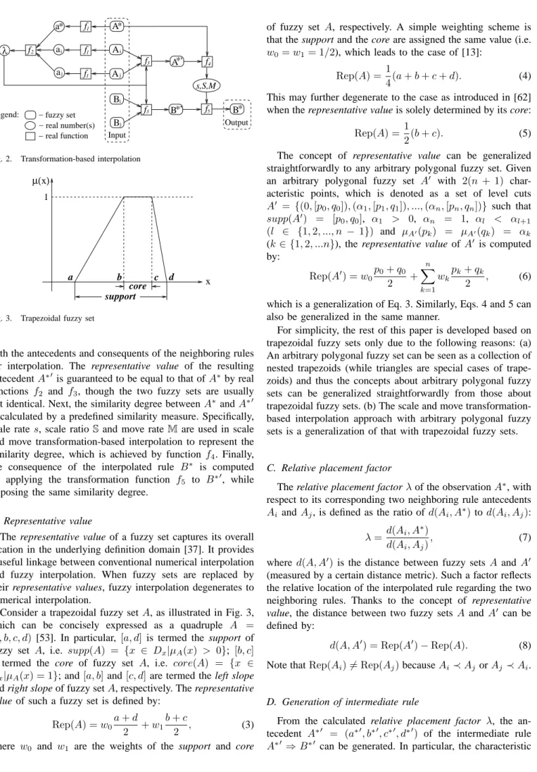
transformation-based fuzzy interpolation. The interpolation process can be illustrated in Fig. 2.
This process is outlined as follows with key concepts
introduced after this overview. Given fuzzy sets Ai, Aj and
A∗, it first uses real numbers a
i, aj and a∗ termed as
representative values, to represent the overall position of Ai,
Aj and A∗ respectively, within the domain of variable x,
mapped by the real functionf1. Then, the relative placement
relation between the observationA∗
and the antecedents (Ai
and Aj) of the two neighboring rules for interpolation is
obtained, which corresponds toλ, termed as relative placement
factor, and which is calculated by the real functionf2. From
this, an intermediate rule A∗′
⇒ B∗′
can be interpolated
f4 f5 λ f2 f1 f1 f1 s,S,M f f 3 Input Output 3
Legend: − fuzzy set real number(s) real function − − a a A A A B B * A*’ *’ B * B a* i j i j j i
Fig. 2. Transformation-based interpolation
1 x x µ( ) c b core support d a
Fig. 3. Trapezoidal fuzzy set
both the antecedents and consequents of the neighboring rules for interpolation. The representative value of the resulting
antecedentA∗′ is guaranteed to be equal to that ofA∗by real
functions f2 and f3, though the two fuzzy sets are usually
not identical. Next, the similarity degree between A∗andA∗′
is calculated by a predefined similarity measure. Specifically,
scale rates, scale ratio Sand move rateM are used in scale
and move transformation-based interpolation to represent the
similarity degree, which is achieved by function f4. Finally,
the consequence of the interpolated rule B∗
is computed
by applying the transformation function f5 to B∗′, while
imposing the same similarity degree.
B. Representative value
The representative value of a fuzzy set captures its overall location in the underlying definition domain [37]. It provides a useful linkage between conventional numerical interpolation and fuzzy interpolation. When fuzzy sets are replaced by their representative values, fuzzy interpolation degenerates to numerical interpolation.
Consider a trapezoidal fuzzy set A, as illustrated in Fig. 3,
which can be concisely expressed as a quadruple A =
(a, b, c, d) [53]. In particular, [a, d] is termed the support of
fuzzy set A, i.e. supp(A) = {x ∈ Dx|µA(x) > 0}; [b, c]
is termed the core of fuzzy set A, i.e. core(A) = {x ∈
Dx|µA(x) = 1}; and[a, b]and[c, d]are termed the left slope
and right slope of fuzzy setA, respectively. The representative
value of such a fuzzy set is defined by:
Rep(A) =w0
a+d
2 +w1
b+c
2 , (3)
where w0 and w1 are the weights of the support and core
of fuzzy set A, respectively. A simple weighting scheme is
that the support and the core are assigned the same value (i.e. w0=w1= 1/2), which leads to the case of [13]:
Rep(A) =1
4(a+b+c+d). (4)
This may further degenerate to the case as introduced in [62] when the representative value is solely determined by its core:
Rep(A) =1
2(b+c). (5)
The concept of representative value can be generalized straightforwardly to any arbitrary polygonal fuzzy set. Given
an arbitrary polygonal fuzzy set A′ with 2(n + 1)
char-acteristic points, which is denoted as a set of level cuts A′
= {(0,[p0, q0]),(α1,[p1, q1]), ...,(αn,[pn, qn])} such that supp(A′
) = [p0, q0], α1 > 0, αn = 1, αl < αl+1 (l ∈ {1,2, ..., n − 1}) and µA′(pk) = µA′(qk) = αk (k∈ {1,2, ...n}), the representative value of A′
is computed by: Rep(A′) =w0 p0+q0 2 + n X k=1 wk pk+qk 2 , (6)
which is a generalization of Eq. 3. Similarly, Eqs. 4 and 5 can also be generalized in the same manner.
For simplicity, the rest of this paper is developed based on trapezoidal fuzzy sets only due to the following reasons: (a) An arbitrary polygonal fuzzy set can be seen as a collection of nested trapezoids (while triangles are special cases of trape-zoids) and thus the concepts about arbitrary polygonal fuzzy sets can be generalized straightforwardly from those about trapezoidal fuzzy sets. (b) The scale and move transformation-based interpolation approach with arbitrary polygonal fuzzy sets is a generalization of that with trapezoidal fuzzy sets.
C. Relative placement factor
The relative placement factorλof the observationA∗, with
respect to its corresponding two neighboring rule antecedents
Ai andAj, is defined as the ratio ofd(Ai, A∗)tod(Ai, Aj):
λ=d(Ai, A ∗ ) d(Ai, Aj) , (7) where d(A, A′
)is the distance between fuzzy sets A andA′
(measured by a certain distance metric). Such a factor reflects the relative location of the interpolated rule regarding the two neighboring rules. Thanks to the concept of representative
value, the distance between two fuzzy sets A andA′ can be
defined by:
d(A, A′
) = Rep(A′
)−Rep(A). (8)
Note thatRep(Ai)6= Rep(Aj)becauseAi≺AjorAj ≺Ai.
D. Generation of intermediate rule
From the calculated relative placement factor λ, the
an-tecedent A∗′
= (a∗′
, b∗′
, c∗′
, d∗′
) of the intermediate rule
A∗′ ⇒B∗′
points of A∗′ are computed as follows: a∗′= (1−λ)a i+λaj b∗′= (1−λ)bi+λbj c∗′= (1−λ)c i+λcj d∗′ = (1−λ)di+λdj (9) which are collectively abbreviated to:
A∗′
= (1−λ)Ai+λAj. (10)
In so doing, the representative value of the calculated A∗′
is guaranteed to be equal to that of the given observation A∗
(refer to [37] for details). Similarly, the consequence of the intermediate rule is generated using the same relative
placement factor λ by analogy to the generation of the antecedent:
B∗′= (1−λ)Bi+λBj. (11)
Note that the interpolated intermediate rule is normal and convex.
E. Firing the intermediate rule
Having generated the intermediate rule, the next step is to execute the rule with the given observation, which is achieved by employing a similarity reasoning mechanism. Suppose that
the interpolated intermediate rule is A∗′
⇒ B∗′
, and that
the observation is A∗. The conclusionB∗ is calculated with
respect to the following intuition:
The more similar A∗
is toA∗′
, the more similarB∗
is toB∗′
. (12) Given two fuzzy sets with the same representative value, the similarity between them is assessed through a process of two transformation steps, namely, scale transformation and
move transformation. In particular, three parameters: scale rate, scale ratio and move rate are introduced to measure
the scales of these two transformations. Scale rate and scale
ratio measure the “fuzziness” difference of the two sets by
comparing the lengths of a certain level cut, while move rate measures the “position” difference by comparing their shifts
on the given level cut. From this, the consequence B∗
can
be obtained by modifying B∗′
with the same scale and move
parameters as used for transformingA∗′
toA∗
. For simplicity, the two transformation steps are jointly represented by an integrated transformation function such that:
T(B∗′, B∗) =T(A∗′, A∗), (13)
which ensures that the degree of the similarity between B∗′
andB∗
is the same as that between A∗′
andA∗
. The details of these transformations and the computation of the scale and move rates are omitted here due to limitations of space, but can be found in [37], [38].
F. Multiple-antecedent rule interpolation
Multiple-antecedent rule interpolation is a generalization of single-antecedent rule interpolation. Given an observation
O: x1 isA∗1x and...andXm isA
∗
mx, (14)
suppose that rules
Ri: If x1 isA1i and...andxmisAmi, theny isBi, Rj: Ifx1is A1j and... andxm isAmj, theny isBj,
(15)
are used for interpolation with respect to the observation O,
which are referred to as that “rules Ri and Rj flank the
observationO”. For simplicity, such two rules will be referred
to as the “neighboring rules” hereafter. Similar to the
single-antecedent rule situation, the neighboring rules Ri and Rj
must satisfy: i)Aki≺Akj orAkj≺Aki,∀k∈ {1,2, ..., m};
ii) Aki A∗kx Akj or Akj A∗kx Aki, ∀k ∈
{1,2, ..., m}; and iii) the distance between the antecedents of
rulesRi andRj is the smallest amongst those of all the rule
pairs in the rule base satisfying i) and ii) at the same time.
Knowing the distance between each pair of fuzzy setsAki
(1 ≤ k ≤ m) and Akj calculated by Eq. 8, the distance
between the antecedents of rules Ri and Rj can be defined
as the Euclidean distance within the input space (though other alternative distance metrics may be used). However, the absolute distances within different dimensions may not be compatible because different attributes have different domains. In order to make them compatible, the normalized attribute distance is defined by:
d′
k=
d(Aki, Akj) maxk−mink
, (16)
where maxk and mink are the maximal and minimal values
in the domain of attribute k, respectively. From this, the
normalized distance d′
between the antecedents of rules Ri
andRj is calculated by:
d′ = 1 m v u u t m X k=1 d′ k 2. (17)
Then, the distancedbetween the antecedents of rules Ri and
Rj is defined as the denormalisation ofd′:
d=d′ v u u t m X k=1 (maxk−mink)2. (18)
Note that if the neighboring rules of Eq. 15 degenerate to those of a single antecedent of Eq. 2, Eq. 18 degenerates to Eq. 8.
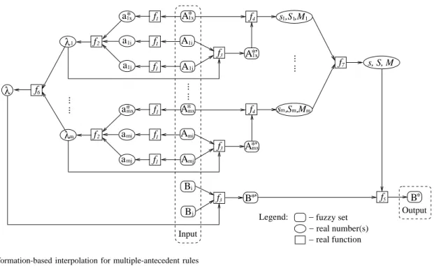
Having known the neighboring rules for interpolation, the
process of deriving the object value B∗ of the consequent
variable y is illustrated in Fig. 4. In this figure, there are
m repeated components which are identical to the core of
the single-antecedent rule interpolation (Fig. 2). Each of these components does exactly the same as the common core of the single-antecedent situation. That is, relative placement factor
λk (1 ≤ k ≤ m) and similarity rates (sk, Sk, Mk) are
calculated from each term of the observation A∗
kx and the
corresponding two fuzzy sets Aki and Akj. Function f6 is
introduced to combine all these λk (k ∈ {1,2, ..., m}) to a
single scaleλ, as isf7to combine all the similarity rates (sk,
Sk,Mk) to (s,S,M). Various combination functions may be
chosen forf6andf7[5], [6]. For instance, the chosen function
f2 f1 f1 f1 f2 f1 f1 f1 f4 f4 1 1 1 s ,S ,M mMm S , s m , f5 − fuzzy set real number(s) real function − − Legend: λ λ1 m ... ... 3 ... ... f3 f3 Input A A1i A 1j 1x Ami f a1x 1i a 1j a mx a ami amj f7 Output ... ... Amj mx A s, S, M B B ’* * A ’* * * 1x A ’*mx * * Bi j B f6 λ
Fig. 4. Transformation-based interpolation for multiple-antecedent rules
The simplest case is the arithmetic average operator:
r= 1 m m X k=1 rk, (19)
where r stands for similarity rates s, S and M or relative
placement factorsλ. This operator will be used in the running
example below.
The combined similarity rate reflects the similarity degree between the observation and the antecedents of the
inter-mediate rule. The conclusion B∗ can then be estimated by
transforming the consequent B∗′
of the intermediate rule via the application of the combined similarity rate, using
transformation function f5: T(B∗′ , B∗ ) =T((A∗ 1x ′ , ...., A∗ mx ′ ),(A1x, ...., Amx)). (20) G. Other implementations
The discussions throughout this paper focus on the scale and move transformation-based approach (due to its basic properties stated previously). However, the work is developed with an aim to suit a variety of intermediate rule-based interpolation approaches, including the following important implementations. The technique of [62] employs the same method for generating intermediate rules as outlined above, but the representative value is restricted to the middle point of core (i.e. Eq. 5). The similarity degree is captured using the so-called lower similarity and upper similarity. By reference to the middle point of the core, a normal and convex fuzzy set can be divided into two parts, namely the lower part and the upper part. The lower similarity measures the difference of the lower parts of two fuzzy sets by comparing the lengths of a certain level cut, and upper similarity does that of the upper parts.
The approach of [13] ensures that the core of each fuzzy set of a created intermediate rule is equal to that of the
corresponding fuzzy set of the resulting interpolated rule. In order to measure the similarity degree between two fuzzy sets with the same core, only their left slopes and right slopes need to be compared. Two transformations, that is, increment
transformation and ratio transformation are utilized for this
purpose, with one aiming to increase the length of a certain level cut of a slope during the transformation, and the other to decrease the length. A group of intermediate rule generation and firing algorithms have also been reported in [2] by means of fuzzy relations and semantic relations. For details of these implementations, refer to the corresponding references given above.
III. MINIMALCANDIDATEGENERATION
In fuzzy reasoning, including fuzzy interpolation, it is possible that more than one object value of a single variable is derived. This implies that certain inconsistencies have been
reached. For example, variablexis used to illustrate a person’s
height. It is possible thatx is tall is held in one situation and
thatx is shortin another, while it is contradictory forx is tall
andx is shortto be held simultaneously in one single
situa-tion, knowing thattall andshort represent two semantically
different object values. Given such an inconsistency, for fuzzy interpolation, unless it is caused by contradictory observations, the method employed is the only cause of contradiction (if the neighboring rules used are presumed to be true).
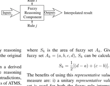
In this work, each pair of neighboring rules is seen as a fuzzy reasoning component which takes a certain number of fuzzy sets as input and produces another fuzzy set as output, as illustrated in Fig. 5. The input is an observation or a previously
inferred result, which is of the form (1) or (14). Rulesi and
j flank the given observation and are of the form (2) for
single-premise, or form (15) for multiple-premise. The result is inferred from the input observation by such two neighboring rules as explained earlier. Accordingly, a contradiction in
j Rule Rule i Fuzzy Component Reasoning
Inputs Outputs Interpolated result previously interpolated result
or Observation
Fig. 5. Fuzzy reasoning component
this context means that at least one of the fuzzy reasoning components that it depends on is defective unless the original given observations are themselves inconsistent.
To efficiently record the dependencies between a derived proposition and its preceding fuzzy interpolative reasoning components, including those which lead to contradictions, ATMS is used here. GDE, which is built on the basis of ATMS, can then be employed to generate minimal faulty reasoning component candidates, with each of which explaining the entire set of current contradictions. A minimal candidate is a possible minimal set of defective components which need to be corrected at one time in order to remove all the contradictions.
A. Contradictions in interpolation
In classical reasoning, at a given time, if two unequal values are derived (or one derived and another observed) for one sin-gle variable, there is a contradiction. The situation is different in fuzzy reasoning, as “unequal” in fuzzy representation is a matter of degree. For fuzzy systems, the concept of contra-diction is replaced by the concept of dissimilarity between the derived logical consequences for any given variable. The degree of matching is frequently used for expressing the extent of similarity between two fuzzy sets. Numerous methods have been proposed to calculate fuzzy matching degrees in the literature [15], [69], which can be typically categorized into two classes: geometric distance-based measures and set
theory-based measures. The former are the extensions of the
classical concept of metric space and the associated distance function, while the latter are built on the basis of set operators,
such as t-norms and t-conorms.
1) Geometric distance-based matching degree: This
ex-tends the Euclidean distance between two points to a fuzzy distance between two fuzzy sets, to express the extent to which the fuzzy sets match. An extensive mathematical literature exists for computing such measures (e.g. [10], [11], [22], [25], [34], [49], [51]). Having defined the representative value of a fuzzy set, the matching degree between two fuzzy sets can be easily calculated. This is because the distance between two fuzzy sets degenerates to the geometric distance between their
representative values. Thus, the matching degree between two
fuzzy sets Ai andAj, denoted asM(Ai, Aj), in the domain
Dx of variablexcan be defined by:
M(Ai, Aj) = 1, ifd(Ai, Aj) =Si=Sj = 0 1− d(Ai,Aj) d(Ai,Aj)+Si +Sj 2 , otherwise (21)
where Sk is the area of fuzzy set Ak. Given a trapezoidal
fuzzy setAk = (a, b, c, d),Sk can be calculated by:
Sk =
1
2[(d−a) + (c−b)]. (22)
The benefits of using this representative value-based matching measure are: i) a unitary representative value of each fuzzy set is used for both the fuzzy rule interpolation phase and the contradiction calculation phase; and ii) the representative
value for each fuzzy set only needs to be calculated once,
saving computational effort.
2) Set theory-based matching degree: An alternative way
to measure the similarity degree between two fuzzy sets is developed from the set theory. This approach is rooted in the assertion that the assessment of similarity may be better described as a comparison of features rather than as a compu-tation of metric distance between points [58]. For instance, in case-based reasoning, the determination of the most relevant (or optimal) case that is to be retrieved is based on the similarity degrees which are usually computed by comparison of the involved features [52]. In the area of pattern recognition, the similarity between an object and a pattern class can be identified also by comparison of features [4]. Similarity among objects is expressed as a linear combination of the measures of their common and distinct features, which degenerates to set operations when special parameters are chosen. A number of fuzzy distance measures have been proposed in the literature as the extensions or generalizations of this concept [14], [27], [28]. Particularly, the matching degree between two fuzzy sets
Ai and Aj, denoted as M(Ai, Aj), in the domain Dx of
variablexcan be defined as:
M(Ai, Aj) = sup x∈Dx
[min(µAi(x), µAj(x))]. (23)
This is in accordance with the implication-based interpretation of fuzzy rules, as opposed to the conjunction-based interpre-tation [29], [30].
Both similarity measures proposed above follow the
prop-erties ofsymmetryandref lexivitywhich are necessary for
any matching degree metric. Thus, a choice may be made according to the given application problem. In particular, the representative value-based similarity measure is sensitive among different pairs of disjoint fuzzy sets, while the set
theory-based is sensitive among different pairs of joint fuzzy
sets.
3) Specification of contradiction: Based on the concept of
matching degree, the degreeβ of a contradiction with respect
to two propositionsP(x is Ai) and P′(x is Aj) is specified
by:
A predefined threshold β0 (0 ≤ β0 ≤1) can be adopted in order to determine those values assigned to a common variable with an unacceptable contradictory degree. A contradiction
is called a β0-contradiction if the corresponding degree of
contradiction β > β0.
In fuzzy interpolation, when two or more values of a common variable are obtained, the degree of contradiction between each pair of values is calculated as above. From this, the following interpretations will be adopted in this paper: (i) β = 0, that is M(Ai, Aj) = 1, which means that the
two propositions P and P′
are not contradictory at all; in
other words, they are totally consistent; (ii) 0 < β ≤ β0,
that is 1 −β0 ≤ M(Ai, Aj) < 1, which means that the
two propositionsP andP′
are slightly contradictory and the degree of contradiction is tolerable in the computation; (iii) β0< β <1, that is 0< M(Ai, Aj)<1−β0, which means
that the two propositionsPandP′ are seriously contradictory
and the degree of contradiction is intolerable; (iv)β = 1, that
is M(Ai, Aj) = 0, which means that the two propositionsP
andP′ are totally contradictory, and not consistent at all.
B. Representation of interpolation concepts in ATMS
In this work, ATMS is used to record the dependency of the interpolated results as well as the contradictions derived from those fuzzy reasoning components. That is, propositions, contradictions and fuzzy interpolative reasoning components are all represented as ATMS nodes. In addition to the so-called datum field [18], which trivially denotes a proposition (including the term “false” to represent inconsistency) or a fuzzy reasoning component, an ATMS node has two other fields: justification and label.
1) Justification: A justification describes how a node is
derivable from other nodes. Each fuzzy reasoning component is assumed to be initially true and may be detected to be false later. For such a node (i.e. an assumption in classical ATMS terms [18]), its justification just assumes itself to be true. For
any given observationO(i.e. a premise [18]), its corresponding
ATMS node has a justification with no antecedent because it is supposed to hold universally, which can be represented as:
⇒O. (25)
Any ATMS node with an inferred proposition (i.e. a derived node [18]), which is obtained through fuzzy interpolative reasoning, can be represented by an ATMS justification as:
O, RiRj ⇒C, (26)
where RiRj stands for the fuzzy reasoning component with
respect to the two neighboring rules Ri andRj (i6=j) that
have been used to infer the outcome C from the observation
O. More generally, a nodeN that is inferred bynother nodes
M1, M2, ...Mn (each of which may be itself a derived node or an observation) by interpolation through two neighboring
rules Ru andRv (u6=v)is denoted by:
M1, M2, ..., Mn, RuRv ⇒N. (27)
In addition, as discussed previously, any two propositions
P (x is Ai) and P′ (x is Aj) are considered contradictory
if Ai andAj are not identical. Due to fuzzy matching, such
contradictions are to a certain degreeβ. Whenβ is not higher
than a given thresholdβ0, the contradictory degree is deemed
acceptable and the two considered propositions are treated as
being consistent in ATMS. Otherwise, aβ0-contradiction is
deduced, which is represented as: P, P′
⇒β0 ⊥. (28)
2) Label and label-updating: A label is a set of
environ-ments each supporting the associated node. An environment contains a minimal set of fuzzy reasoning components that jointly entail the node from an observation, thereby describing how the node depends on those fuzzy reasoning
compo-nents. An environment is said to be β0-inconsistent if β0
-contradiction is derivable propositionally from the environ-ment and a given justification. An environenviron-ment is said to be (1−β0)-consistent if it is not β0-inconsistent.
The label of each node is guaranteed to be (1 −
β0)-consistent, sound, minimal and complete, except that the
label of the special “false” node isβ0-inconsistent rather than
(1−β0)-consistent. The interpretation of these properties is summarized as follows:
• (1−β0)-consistency means that all environments in the
label are at least(1−β0)-consistent;
• (1−β0)-soundness indicates that the node is derivable
from each environment in the label at least to the
consis-tent degree of(1−β0);
• (1−β0)-minimality states that the removal of any
ele-ment from any environele-ment will cause the node to be underivable from that environment and hence violating
the label’s(1−β0)-soundness;
• (1 − β0)-completeness implies that every
(1−β0)-consistent environment, from which the node is derivable, is a superset of a certain environment in the
label. In other words, all minimal (1−β0)-consistent
environments of the subject node are held within the label.
The label-updating algorithm of the ATMS ensures that the above four properties are held. The extended algorithm for label-updating in this work is exactly the same as the original given in [18], except that the environments of a proposition
are now at least (1−β0)-consistent rather than 1-consistent
and that the environments of a contradiction are at least
β0-inconsistent rather than1-inconsistent (i.e. a contradiction
is at least β0-contradictory rather than 1-contradictory). In
particular, the label of the special “false” node gathers all
β0-inconsistent environments. Whenever aβ0-contradiction is
detected, each environment in its label is added into the label of the specific “false” node and all such environments and their supersets are removed from the label of every other node. Also, any such an environment which is a superset of another is removed from the label of the node “false”.
Accordingly, the concept of an ATMS context with respect to a (1 −β0)-consistent environment, is herein defined by the collection of both the assumptions contained within this environment and all those nodes that can be derived from these assumptions. Of course, these derived nodes can not be
β0-inconsistent because they are deduced from a (1−β0 )-consistent environment. Note that there are a number of fuzzy extensions of de Kleer’s ATMS in the literature, such as [7], [8], [26], [55]. All these extensions introduce truth values into ATMS. They may be of great significance when this work is extended to deal with truth values of propositions or rules, but are beyond the scope of this paper.
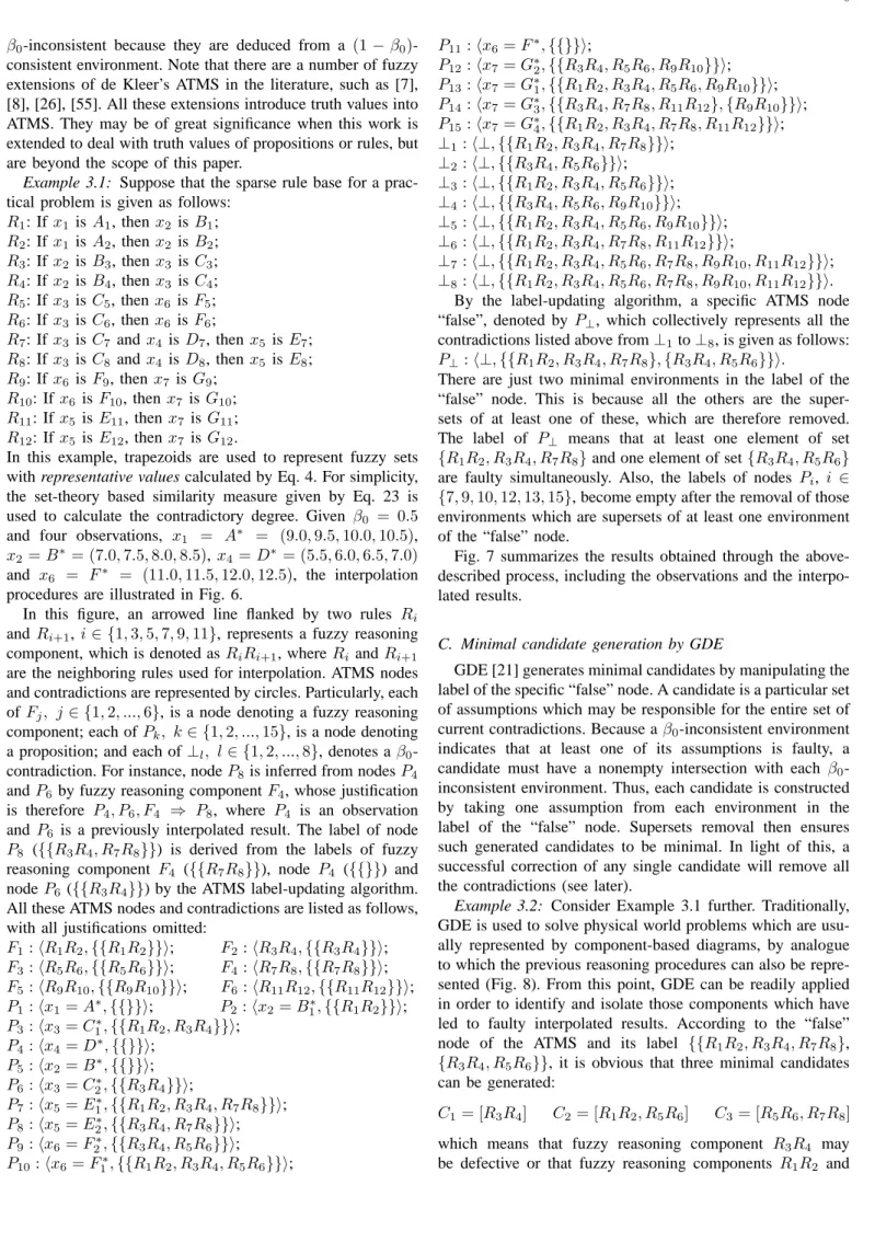
Example 3.1: Suppose that the sparse rule base for a
prac-tical problem is given as follows:
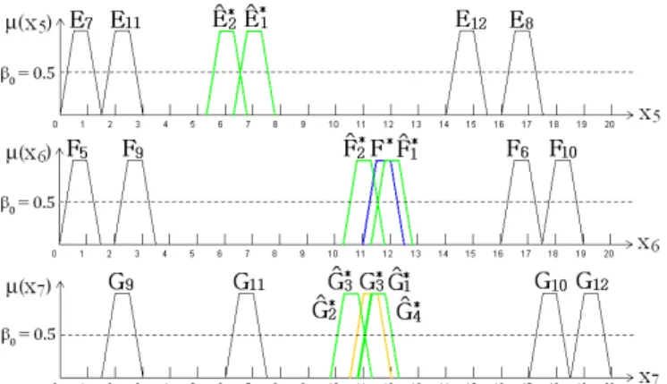
R1: If x1 isA1, thenx2 isB1; R2: If x1 isA2, thenx2 isB2; R3: If x2 isB3, thenx3 isC3; R4: If x2 isB4, thenx3 isC4; R5: If x3 isC5, thenx6 isF5; R6: If x3 isC6, thenx6 isF6; R7: If x3 isC7 andx4 isD7, thenx5 is E7; R8: If x3 isC8 andx4 isD8, thenx5 is E8; R9: If x6 isF9, thenx7is G9; R10: If x6is F10, thenx7 is G10; R11: If x5is E11, thenx7 isG11; R12: If x5is E12, thenx7 isG12.
In this example, trapezoids are used to represent fuzzy sets with representative values calculated by Eq. 4. For simplicity, the set-theory based similarity measure given by Eq. 23 is
used to calculate the contradictory degree. Given β0 = 0.5
and four observations, x1 = A∗ = (9.0,9.5,10.0,10.5),
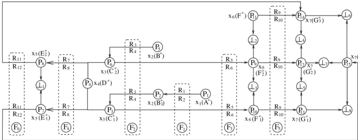
x2=B∗ = (7.0,7.5,8.0,8.5),x4=D∗= (5.5,6.0,6.5,7.0) and x6 = F∗ = (11.0,11.5,12.0,12.5), the interpolation procedures are illustrated in Fig. 6.
In this figure, an arrowed line flanked by two rules Ri
andRi+1,i∈ {1,3,5,7,9,11}, represents a fuzzy reasoning
component, which is denoted as RiRi+1, whereRiandRi+1
are the neighboring rules used for interpolation. ATMS nodes and contradictions are represented by circles. Particularly, each of Fj, j∈ {1,2, ...,6}, is a node denoting a fuzzy reasoning
component; each ofPk, k∈ {1,2, ...,15}, is a node denoting
a proposition; and each of⊥l, l∈ {1,2, ...,8}, denotes aβ0
-contradiction. For instance, nodeP8is inferred from nodesP4
andP6 by fuzzy reasoning componentF4, whose justification
is therefore P4, P6, F4 ⇒ P8, where P4 is an observation
and P6 is a previously interpolated result. The label of node
P8 ({{R3R4, R7R8}}) is derived from the labels of fuzzy
reasoning component F4 ({{R7R8}}), node P4 ({{}}) and
nodeP6 ({{R3R4}}) by the ATMS label-updating algorithm.
All these ATMS nodes and contradictions are listed as follows, with all justifications omitted:
F1:hR1R2,{{R1R2}}i; F2:hR3R4,{{R3R4}}i; F3:hR5R6,{{R5R6}}i; F4:hR7R8,{{R7R8}}i; F5:hR9R10,{{R9R10}}i; F6:hR11R12,{{R11R12}}i; P1:hx1=A∗,{{}}i; P2:hx2=B∗1,{{R1R2}}i; P3:hx3=C1∗,{{R1R2, R3R4}}i; P4:hx4=D∗,{{}}i; P5:hx2=B∗,{{}}i; P6:hx3=C2∗,{{R3R4}}i; P7:hx5=E1∗,{{R1R2, R3R4, R7R8}}i; P8:hx5=E2∗,{{R3R4, R7R8}}i; P9:hx6=F2∗,{{R3R4, R5R6}}i; P10:hx6=F1∗,{{R1R2, R3R4, R5R6}}i; P11:hx6=F∗,{{}}i; P12:hx7=G∗2,{{R3R4, R5R6, R9R10}}i; P13:hx7=G∗1,{{R1R2, R3R4, R5R6, R9R10}}i; P14:hx7=G∗3,{{R3R4, R7R8, R11R12},{R9R10}}i; P15:hx7=G∗4,{{R1R2, R3R4, R7R8, R11R12}}i; ⊥1:h⊥,{{R1R2, R3R4, R7R8}}i; ⊥2:h⊥,{{R3R4, R5R6}}i; ⊥3:h⊥,{{R1R2, R3R4, R5R6}}i; ⊥4:h⊥,{{R3R4, R5R6, R9R10}}i; ⊥5:h⊥,{{R1R2, R3R4, R5R6, R9R10}}i; ⊥6:h⊥,{{R1R2, R3R4, R7R8, R11R12}}i; ⊥7:h⊥,{{R1R2, R3R4, R5R6, R7R8, R9R10, R11R12}}i; ⊥8:h⊥,{{R1R2, R3R4, R5R6, R7R8, R9R10, R11R12}}i. By the label-updating algorithm, a specific ATMS node
“false”, denoted by P⊥, which collectively represents all the
contradictions listed above from⊥1to⊥8, is given as follows:
P⊥:h⊥,{{R1R2, R3R4, R7R8},{R3R4, R5R6}}i.
There are just two minimal environments in the label of the “false” node. This is because all the others are the super-sets of at least one of these, which are therefore removed.
The label of P⊥ means that at least one element of set
{R1R2, R3R4, R7R8}and one element of set{R3R4, R5R6}
are faulty simultaneously. Also, the labels of nodes Pi, i ∈
{7,9,10,12,13,15}, become empty after the removal of those
environments which are supersets of at least one environment of the “false” node.
Fig. 7 summarizes the results obtained through the above-described process, including the observations and the interpo-lated results.
C. Minimal candidate generation by GDE
GDE [21] generates minimal candidates by manipulating the label of the specific “false” node. A candidate is a particular set of assumptions which may be responsible for the entire set of
current contradictions. Because aβ0-inconsistent environment
indicates that at least one of its assumptions is faulty, a
candidate must have a nonempty intersection with each β0
-inconsistent environment. Thus, each candidate is constructed by taking one assumption from each environment in the label of the “false” node. Supersets removal then ensures such generated candidates to be minimal. In light of this, a successful correction of any single candidate will remove all the contradictions (see later).
Example 3.2: Consider Example 3.1 further. Traditionally,
GDE is used to solve physical world problems which are usu-ally represented by component-based diagrams, by analogue to which the previous reasoning procedures can also be repre-sented (Fig. 8). From this point, GDE can be readily applied in order to identify and isolate those components which have led to faulty interpolated results. According to the “false”
node of the ATMS and its label {{R1R2, R3R4, R7R8},
{R3R4, R5R6}}, it is obvious that three minimal candidates
can be generated:
C1= [R3R4] C2= [R1R2, R5R6] C3= [R5R6, R7R8]
which means that fuzzy reasoning component R3R4 may
6 R R 5 6 R R 5 6 F3 3 R 10 F5 5 7 8 Reasoning component 5 P1 Reasoning component 1 R1 R2 F2 R R 3 4 R R 3 4 F6 R11 R12 R11 R12 R R R R 7 8 7 8 F4 1 R R R R P x P 2 4 9 9 10 10 9 R x P 9 10 P P12 13 Px Reasoning component 3 15 P11 14 6 7 6 7 F1 Reasoning Reasoning Reasoning
component 6 component 4 component 2 P P P P2 3 5 6 P8 5 x x5 P7 x3 x3 2 x 2 (E ) 1 1 (B )* 2 1 * (C ) (C ) * * (E )* x1(A ) 1 2 (F ) (F ) * * * 4 (G )* 7 x (F )* 6 x * (B ) 2 x x7(G )3* * 2 (G ) x P4x4(D )* 1 (G )*
Fig. 6. Discrepancy records in ATMS
R R21 R R3 4 R R1211 R R9 10 R R7 8 R R5 6 Component F Component F Component F Component F 4 x x3 x5 x6 x7 x2 1 x 5 3 4 6 Component F1 Component F2
Fig. 8. Component-based representation of the running example
Fig. 7. Fuzzy sets involved in the example
R5R6 orR5R6andR7R8 may both be defective at the same
time. This result can be better understood by examining the following:
• By ⊥1, at least one element of{R1R2, R3R4, R7R8} is
faulty;
• By⊥2, at least one element of{R3R4, R5R6} is faulty;
• By ⊥3, at least one element of{R1R2, R3R4, R5R6} is
faulty;
• By⊥4, at least one element of{R3R4, R5R6, R9R10}is
faulty;
• By ⊥5, at least one element of
{R1R2, R3R4, R5R6, R9R10}is faulty;
• By ⊥6, at least one element of
{R1R2, R3R4, R7R8, R11R12}is faulty;
• By ⊥7 or ⊥8, at least one element of
{R1R2, R3R4, R5R6, R7R8, R9R10, R11R12} is faulty. What GDE deduces is that at least one of the following
three sets of fuzzy reasoning components is faulty, {R3R4}
or {R1R2, R5R6} or {R5R6, R7R8}. The set {R3R4} is
considered as a candidate because R3R4 belongs to every
contradiction given above and if it is faulty, all these seven
assertions are explained. Similarly, the set {R1R2, R5R6} is
considered as a candidate because if R1R2 and R5R6 are
faulty simultaneously, they jointly explain all these assertions
due to at least one element of {R1R2, R5R6} belonging to
each conflict listed above. The set {R5R6, R7R8} is also
considered as a candidate for the same reason. Any other candidate is a superset of at least one of these three candidates and thus removed.
R3R4 is defective means that any interpolated rule whose
antecedent is flanked by the antecedents ofR3andR4is faulty
and needs to be modified. That fuzzy reasoning components
R1R2 and R5R6 are defective at the same time means that
those interpolated rules whose antecedents are flanked by the
antecedents of R1 and R2, and by those of R5 and R6,
are faulty and need to be modified simultaneously. A similar implication exists given that fuzzy reasoning components
R5R6andR7R8 are defective. This leads to the development
of the following procedure for modification of the identified faulty fuzzy reasoning components.
IV. CANDIDATEMODIFICATION
Having described the method for minimal candidate gen-eration, this section deals with how to correct such defective fuzzy reasoning components. It exploits the presumption that any observed inconsistencies are dependent upon the found faults.
A. Consistency restoring algorithm
Since each single candidate explains the entire set of current contradictions, consistency can be restored by successfully correcting any single candidate. A candidate of the smallest cardinality is the easiest to be modified. Therefore, the smallest candidate in cardinality is always the one to be modified first. However, there are still situations in which more than one can-didate have the same size. In this case, the algorithm breaks the tie at random. An alternative way to prioritize the candidates is through the use of the degree of contradiction. Obviously, the higher the threshold taken to detect the contradictory degree, the less sensitive the candidate generation procedure and thus, the fewer candidates that may be generated. Also, the higher the degree of contradiction caused by a candidate, the more likely the candidate to be the actual culprit.
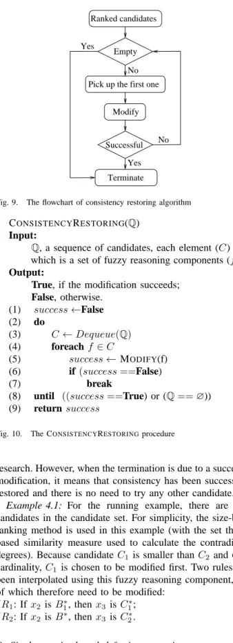
Given a set of ranked candidates, the consistency restoring algorithm tries to correct the candidates one by one until a candidate succeeds (or all fail). For the current working candidate, the algorithm tries to correct each of its defective fuzzy reasoning components and propagate the modification to all the interpolated rules which depend on this defective component by the method to be given in the next section. If the modification is successful, that is all the contradictions have been removed through the correction of all interpolated rules involved in the candidate, the algorithm terminates; otherwise, the algorithm tries the next highest ranked candidate. The flowchart of the algorithm is shown in Fig. 9 and the algorithm
itself is outlined in Fig. 10, where MODIFY(f) is the
modifi-cation procedure for a single fuzzy reasoning component (f). As indicated above, the algorithm terminates under two situations. When the termination is caused by an empty candidate set, it means that the modification fails and the proposed modification method is not suitable for the given problem. This implies that the detected inconsistency may have been caused by incorrect observations or incorrect rules originally given, which have mistakenly been presumed to be true. Further modifications in this case remain for future
Empty
Modify Pick up the first one
Ranked candidates Terminate Successful No No Yes Yes
Fig. 9. The flowchart of consistency restoring algorithm
CONSISTENCYRESTORING(Q)
Input:
Q, a sequence of candidates, each element (C) of
which is a set of fuzzy reasoning components (f).
Output:
True, if the modification succeeds; False, otherwise. (1) success←False (2) do (3) C←Dequeue(Q) (4) foreachf ∈C (5) success←MODIFY(f) (6) if (success==False) (7) break
(8) until ((success==True) or (Q==∅)) (9) returnsuccess
Fig. 10. The CONSISTENCYRESTORINGprocedure
research. However, when the termination is due to a successful modification, it means that consistency has been successfully restored and there is no need to try any other candidate.
Example 4.1: For the running example, there are three
candidates in the candidate set. For simplicity, the size-based ranking method is used in this example (with the set theory-based similarity measure used to calculate the contradictory
degrees). Because candidateC1 is smaller thanC2 andC3 in
cardinality,C1 is chosen to be modified first. Two rules have
been interpolated using this fuzzy reasoning component, both of which therefore need to be modified:
IR1: Ifx2 isB1∗, thenx3 is C1∗;
IR2: Ifx2 isB∗, thenx3 is C2∗.
B. Single-premise-based defective reasoning component cor-rection
Inconsistencies result from the failure of interpolation (un-less observations and/or original rules have been incorrectly given, which are beyond the scope of this paper). The reason for such a failure is that the same relative placement
of an interpolated rule. That is, the interpolation presumes that the relationship between the antecedent variable and the consequent variable is linear. An intuitive way to address this issue is to shift the representative value of the consequence of a culprit reasoning rule within the interval constructed by the representative values of the two consequences of the neighboring rules that were used for interpolation. This helps to explain all other propositions in the context. In so doing, the consequent value of the computed intermediate rule is changed with respect to the change of the representative value of the consequence of the culprit interpolated rule. However, both move and scale rates that are generated by measuring the transformation from the antecedent of the intermediate rule to the antecedent of the interpolated rule remain intact. They are used to transform the consequence of the intermediate rule to the consequence of the modified interpolated rule. This ensures that the similarity between the consequence of the intermediate rule and the consequence of the modified interpolated rule keeps the same as that between the antecedent of the intermediate rule and the antecedent of the interpolated rule.
Based on these considerations, a set of simultaneous equa-tions can be set up regarding all the interpolated rules which are dependent on the same defective fuzzy reasoning com-ponent, in order to modify their consequent values. The modification is carried out such that their corresponding
propo-sitions are (1−β0)-consistent with the current context. The
solution of these simultaneous equations forms the result of
the modification. For convenience, letBb∗denote the modified
consequence of a culprit interpolated rule A∗⇒B∗, andBb∗′
andλBb∗ denote the corresponding modified intermediate rule
consequence and the relative placement factor ofBb∗
, respec-tively. The following sub-sections describe the requirements that the modification should satisfy and their reasons.
1) Unique correction rate for rules interpolated from the same defective reasoning component: There may be more
than one interpolated rule dependent on the same defective fuzzy reasoning component. If an interpolated rule is altered because it depends on a defective fuzzy reasoning component, the same must also be applied to all other interpolated rules which depend on the same fuzzy reasoning component.
In this research, all those rules initially provided in the sparse rule base for interpolation are assumed to be fixed and true, and are referred to as base rules. Naturally, the more similar any two rules are to each other, the closer the values of the attributes involved in these rules. Therefore, the interpolated rule whose antecedent is located farthest from both antecedents of a pair of base neighboring rules is the one that is most dissimilar to these neighboring rules. Thus, this farthest rule should be chosen for initial modification. In other words, the rule antecedent which sits nearest the middle of the neighborhood of the two base rules is the one most likely to be wrong and needs to be modified the most. Any other interpolated rules dependent on the same fuzzy reasoning component can then be modified with reference to the modification of this one.
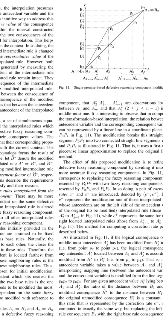
Suppose that the neighboring rulesA1⇒B1andAn⇒Bn
are the two base rules used by a defective fuzzy reasoning
A A A A A p0 p1 p2 p3 p4 p5 6 p p7 x 1 1 >B = A =1 j+1 n k j i 1 n A ==>Bn y i j A ,..., A ,..., A A ,..., A ,..., Ak n * * * B B B B B B B B n k k j j i i 1 * * * * * * * * * *
Fig. 11. Single-premise-based defective reasoning component modification
component, that A∗
2, A∗3, ..., A∗n−1 are observations located
between A1 and An, and that Aj∗ (2 ≤ j ≤ n−1) is the
middle-most one. It is interesting to observe that in computing the transformation-based interpolation, the relation between an antecedent variable and the corresponding consequent variable can be represented by a linear line in a coordinate plane (line
P0P7 in Fig. 11). The modification breaks this straight line
segmentP0P7into two connected straight line segmentsP0P5
andP5P7as illustrated in Fig. 11. That is, it uses a first-order
piecewise linear approximation to replace the original linear method.
The effect of this proposed modification is to refine the defective fuzzy reasoning component by dividing it into two more accurate fuzzy reasoning components. In Fig. 11, this corresponds to replacing the fuzzy reasoning component
rep-resented byP0P7 with two fuzzy reasoning components
rep-resented byP0P5 andP5P7. In so doing, a pair of correction
rates c− and c+ are introduced, denoted by (c−, c+). Here,
c− represents the modification rate of those interpolated rules
whose antecedents are on the left side of the antecedent value of the original (to be modified) interpolated rule (those from A∗
2toA∗j−1in Fig. 11), whilec+represents the same for those
right located interpolated rules (those from A∗
j+1 toA∗n−1 in
Fig. 11). The method for computing a correction rate pair is described below.
As illustrated in Fig. 11, if the logical consequence of the
middle-most antecedentA∗
j has been modified fromB
∗
j toBb
∗
j
(i.e. from point p2 to point p5), the logical consequence of
any antecedentA∗
i located betweenA1andA∗j is accordingly
modified from B∗
i to Bb
∗
i (i.e. from p1 top4). That is, if the
antecedent variable takes a value between A1 and A∗j, the
interpolating mapping line (between the antecedent variable and the consequent variable) is modified from the line segment
p0p2top0p5. For any given antecedent valueA∗i lying between
A1 and A∗j, the ratio of the distance between B1 and the
modified consequence Bb∗
i to the distance between B1 and
the original unmodified consequence B∗
i is a constant. It is
this ratio that is represented by the correction ratec−
.c+ is
computed in exactly the same way, but replacing the left base
Formally, the correction rate pair (c−, c+)are defined as: c−=d(B1,Bb ∗ j) d(B1, Bj∗); c += d(Bb ∗ j, Bn) d(B∗ j, Bn) . (29)
From (7) and (29), it follows that: c− =d(B1,Bbj∗) d(B1,Bj∗) = d(B1,Bb∗ j) d(B1,Bn) d(B1,B∗ j) d(B1,Bn) =λBb∗j λB∗ j ; c+ =d(Bbj∗,Bn) d(B∗ j,Bn)= d(B1,Bn)−d(B1,Bb∗j) d(B1,Bn)−d(B1,B∗j) = d(B1,Bn)−d(B1,Bb∗ j) d(B1,Bn) d(B1,Bn)−d(B1,B∗ j) d(B1,Bn) = 1− d(B1,Bb∗ j) d(B1,Bn) 1−d(B1,B ∗ j) d(B1,Bn) = 1−λBb∗ j 1−λB∗ j . (30)
For any given antecedent A∗
i (2 ≤ i ≤ j−1), which is
located on the left side ofA∗
j, its consequenceB
∗
i is modified
to Bb∗
i, whose corresponding relative placement factor λBb∗
i satisfies: λBb∗ i =λB ∗ i ·c − . (31)
Similarly, for any antecedentA∗
k(j+1≤k≤n−1), which is
on the right side ofA∗
j, the corresponding relative placement
factor λBb∗
k of its modified consequence
b B∗ k satisfies: 1−λBb∗ k= (1−λB ∗ k)·c +. (32)
Example 4.2: Continue the running example. Because
fuzzy setB∗
1 is located nearer the middle thanB
∗
, the culprit
interpolated rule IR1 will be modified first. Suppose that the
relative placement factor of the modified consequence isλCb∗
1.
Then, the correction rate pair are: c− R3R4= λCb∗ 1 λC∗ 1 ; c+R3R4 =1−λCb1∗ 1−λC∗ 1 .
Accordingly, IR2 should be modified with respect to the
generated correction rate pair (c−
R3R4, c
+
R3R4). The relative
placement factor λCb∗
2 of the modified consequence satisfies:
λCb∗ 2 =λC ∗ 2 ·c − R3R4.
The modified interpolated rule consequences Cb∗
1 andCb2∗ can thus be expressed as follows:
b C∗ 1′= (1−λCb∗ 1)C3+λCb1∗C4; b C∗ 2 ′ = (1−λCb∗ 2)C3+λCb2∗C4; T(Cb∗ 1 ′ ,Cb∗ 1) =T(B ∗ 1 ′ , B∗ 1); T(Cb∗ 2 ′ ,Cb∗ 2) =T(B ∗′ , B∗ ).
2) Consistency of modified propositions: This requirement
ensures that the consequence of each modified interpolated
rule is at least (1−β0)-consistent with the current context.
In general, suppose that m object values A1, A2, ..., Am are
obtained for variable x. If they are (1−β0)-consistent, the
matching degree between any pair of these object values
is not higher than the given β0. In accordance with the
concept of contradictory degree (as introduced previously), this requirement can be expressed as follows:
max(1−M(Ai, Aj))≤β0, (33)
where i, j∈ {1,2, ..., m}(i6=j).
Particularly, in the case of using the set theory-based similarity measure, if the intersection point between two fuzzy
sets is lower thanβ0, the contradictory degree between them
is higher than β0. There is an equivalent way to represent a
β0-contradiction by usingβ0-cut due to the convexity of the
fuzzy sets considered herein. If the intersection of β0-cuts of
two fuzzy sets is empty, the contradictory degree between them
is higher thanβ0. This indicates that the contradictory degree
of fuzzy sets concerning a common variable can be calculated according to their membership functions. Therefore, Eq. 33 can be simplified as follows:
m
\
i=1
(Ai)β0 6=∅, (34)
where (Ai)β0 denotes theβ0-cutof fuzzy setAi.
Example 4.3: For the running example, fuzzy setsCb∗
1 and
b
C∗
2 must satisfy the following constraints with respect to this
requirement:
1−M(Cb∗
1,Cb
∗
2)≤β0.
Specifically, if the set theory-based similarity measure given by Eq. 23 is used for this example, the requirement can be expressed as follows:
(Cb∗
1)β0∩(Cb
∗
2)β06=∅.
3) Consistency over modified proposition propagation:
Ev-ery modified value of a given variable is propagated through all possible subsequent interpolations that depend on that variable, as dictated by the dependencies recorded by the ATMS. The corresponding propositions of such updated values are required
to be(1−β0)-consistent. The propagation process follows the
standard transformation-based interpolation approach strictly.
For simplicity, let function I(A∗
i, RlRr) =Bi∗ denote the
transformation-based interpolation from the antecedent fuzzy
set A∗
i to the consequent value B
∗
i, based on the fuzzy
reasoning component involving the neighboring rules Rl and
Rr. Suppose thatmobject valuesA∗1, A∗2, ..., A∗mof variablex
are modified which are located between the antecedent values
of rules Rl and Rr, that the corresponding modified object
values of variable y are B∗
i, i ∈ {1,2, ..., m}, and that n
object values Bl, l ∈ {1,2, ..., n}, of variable y are already
obtained by one way or another. If the modified consequences
b
B∗
i are all (1−β0)-consistent, then they must satisfy:
b B∗ i =I(Ab ∗ i, RlRr), max(1−M(Bb∗ u,Bb ∗ v))≤β0, max(1−M(Bb∗ i, Bl))≤β0, max(1−M(Bp, Bq))≤β0, (35) where u, v∈ {1,2, ..., m}(u6=v); p, q∈ {1,2, ..., n}(p6=q).
Specifically, if the set theory-based similarity measure given by Eq. 23 is used, this can be simplified as follows:
b B∗ i =I(Ab ∗ i, RlRr); mT i=1 (Bb∗ i)β0 TTn l=1 (Bl)β0 6 =∅. (36)
The above discussion addresses the situation where modified proposition propagation is restricted to single-antecedent rules.
This can be readily generalized to multiple-antecedent rules.
Let function I((A∗
i, B
∗
i, C
∗
i, ...), RlRr) = Zi∗ denote the transformation-based interpolation from the antecedent fuzzy
sets (A∗
i, B
∗
i, C
∗
i, ...) to the consequent value Z
∗
i, based on
the fuzzy reasoning component involving neighboring rulesRl
andRr. The consequenceZi∗needs to be accordingly modified
if any fuzzy set of (A∗
i, B
∗
i, C
∗
i, ...) has been modified such
that the modified (A∗
i, B
∗
i, C
∗
i, ...) is flanked by the
neigh-boring rules Rl andRr. If the modified consequences are all
(1−β0)-consistent, the contradictory degree of every pair of fuzzy sets with respect to the consequent variable must be less
than or equal to β0, no matter whether they are modified or
not.
Example 4.4: Continue the running example, the modified
fuzzy setsCb∗
1 andCb
∗
2 of variablex3need to be propagated in
order to modify the subsequent variablesx5,x6andx7. Since
the set theory-based similarity measure has been used in this example previously, the propagated object values of variable
x5 must satisfy the following equations simultaneously:
b E∗ 1 =I((Cb1∗, D∗), R7R8); b E∗ 2 =I((Cb2∗, D∗), R7R8); (Eb∗ 1)β0∩(Eb ∗ 2)β0 6=∅.
Similarly, for the object values of variable x6, they must
satisfy: b F∗ 1 =I(Cb1∗, R5R6); b F∗ 2 =I(Cb2∗, R5R6); (Fb∗ 1)β0∩(Fb ∗ 2)β0∩(F ∗) β0 6=∅.
Also, for the object values of variable x7, the following
equations need to be satisfied:
b G∗ 1=I(Fb ∗ 1, R9R10); b G∗ 2=I(Fb ∗ 2, R9R10); b G∗ 3=I(Eb ∗ 2, R11R12); b G∗ 4=I(Eb ∗ 1, R11R12); ∩4j=1(Gb ∗ j)β0∩(G ∗ 3)β0 6=∅.
4) Combination of correction requirement criteria: As
de-scribed above, each requirement induces a set of constraining equations over the interpolation. For a detected inconsistency, all such induced equations must be satisfied simultaneously. If there exists at least one solution for these equations, the candi-date has been modified successfully. Otherwise, this candicandi-date is discarded and the next one of the smallest cardinality will be tried as indicated in the algorithm given in Section IV-A.
Example 4.5: For the running example, with respect to
can-didateC1, no solution is arrived at by solving all the equations
listed above simultaneously, which means the modification to
C1 has failed. Therefore, candidate C1 is discarded and C2
is then taken for tentative modification, but the modification
to C2 also fails (the derivation of this is omitted here due
to space limitations). Thus C3 needs to be modified. Notice
that there are multiple-premise rules involved in candidateC3,
the modification of which is not covered by the approach introduced above. However, the present approach is readily extendable to deal with this, which is introduced in the next subsection. p3 x3 x p p1 =>C1 x2 A A p i A A k n j D k D i D 1 5 2 j n n A , B ==>Cn n (A ,B n,C )n j Bi ) 1 C , 1 B , 1 (A 0 pA ,B =1 1 j B k B n B k i C C C C C C C n * k * j * i * * * * * * * * *
Fig. 12. Multiple-premise-based defective reasoning component modification
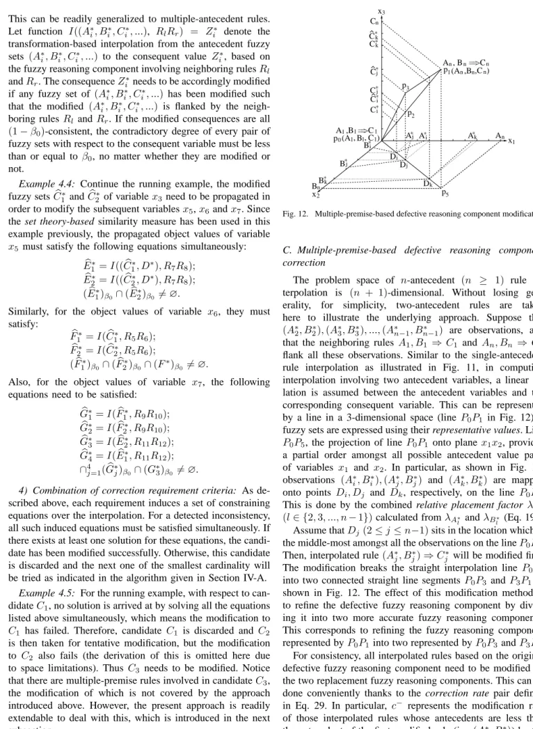
C. Multiple-premise-based defective reasoning component correction
The problem space of n-antecedent (n ≥ 1) rule
in-terpolation is (n + 1)-dimensional. Without losing
gen-erality, for simplicity, two-antecedent rules are taken
here to illustrate the underlying approach. Suppose that (A∗
2, B2∗),(A∗3, B3∗), ...,(A∗n−1, Bn∗−1) are observations, and
that the neighboring rules A1, B1 ⇒ C1 and An, Bn ⇒ Cn
flank all these observations. Similar to the single-antecedent rule interpolation as illustrated in Fig. 11, in computing interpolation involving two antecedent variables, a linear re-lation is assumed between the antecedent variables and the corresponding consequent variable. This can be represented
by a line in a 3-dimensional space (line P0P1 in Fig. 12) if
fuzzy sets are expressed using their representative values. Line
P0P5, the projection of line P0P1 onto plane x1x2, provides
a partial order amongst all possible antecedent value pairs
of variables x1 and x2. In particular, as shown in Fig. 12,
observations (A∗ i, B ∗ i),(A ∗ j, B ∗ j) and (A ∗ k, B ∗ k) are mapped
onto points Di, Dj and Dk, respectively, on the line P0P5.
This is done by the combined relative placement factor λC∗
l
(l∈ {2,3, ..., n−1})calculated fromλA∗
l andλBl∗ (Eq. 19).
Assume thatDj(2≤j ≤n−1)sits in the location which is
the middle-most amongst all the observations on the lineP0P5.
Then, interpolated rule(A∗
j, B
∗
j)⇒C
∗
j will be modified first.
The modification breaks the straight interpolation line P0P1
into two connected straight line segmentsP0P3 andP3P1 as
shown in Fig. 12. The effect of this modification method is to refine the defective fuzzy reasoning component by divid-ing it into two more accurate fuzzy reasondivid-ing components. This corresponds to refining the fuzzy reasoning component
represented byP0P1into two represented byP0P3andP3P1.
For consistency, all interpolated rules based on the original defective fuzzy reasoning component need to be modified by the two replacement fuzzy reasoning components. This can be done conveniently thanks to the correction rate pair defined
in Eq. 29. In particular, c−
represents the modification rate of those interpolated rules whose antecedents are less than
the antecedent of the first modified rule (i.e.(A∗
j, B
∗