Time-optimal Motion Planning for n-DOF Robot Manipulators using a
Path-Parametric System Reformulation*
Robin Verschueren
1, Niels van Duijkeren
2, Jan Swevers
2, Moritz Diehl
1Abstract— Time-optimal motion planning for robotic manip-ulators consists of moving the robot along a path in Cartesian space as fast as possible. In contrast to time-optimal path fol-lowing, small deviations from a predefined path are acceptable and can be exploited to further reduce the overall motion time. In this paper, we present a new method to compute time-optimal motionsaround a path. By employing an appropriate change of variables for the robot dynamics to path coordinates, geometric constraints enter the optimal control formulation in a convenient way. The reformulation of the robot dynamics and the path constraints is shown with numerical examples.
I. INTRODUCTION
Time-optimal motion is of significant importance for max-imizing the productivity of robot systems. Frequently, the essence of a task for a robot is described by the path it should follow. Examples include control of CNC machines, welding robots, but also control of autonomous aerial, land, under-water vehicles. From previous work we learn that generating time-optimal motion starting from a given geometric path can be beneficial. The operator can choose a path that ensures collision avoidance and satisfies other geometric constraints in advance. Given a fixed path in the configuration space of the robot (which may require an inverse kinematics step), the remainder of the trajectory generation problem consists of the significantly simpler step of choosing the optimal timing where to be when on the given path [6], [14]. We will call this thedecoupledapproach to time-optimal motion generation. Recent online approaches to path following go one step further and consider a geometric path solely as reference and generate an optimal feedback law that decides on both the timing and the distance to the reference using a nonlinear model predictive control (NMPC) approach [9], [13].
The geometric path in the workspace of the robot may not be completely strict and, in fact, limited deviations may be perfectly acceptable, for instance in tasks with a certain
*This research benefits from ERC-HIGHWIND (259 166), FP7-ITN-TEMPO (607 957), and H2020-ITN-AWESCO (642 682), K.U.Leuven-BOF PFV/10/002, Center-of-Excellence Optimization in Engineering (OPTEC), and the Belgian Programme on Interuniversity Attraction Poles, initiated by the Belgian Federal Science Policy Office (DYSCO). Robin Verschueren and Niels van Duijkeren are fellows of the TEMPO FP7 Initial Training Network.
The authors would like to thank ABB Sweden for supplying us with useful information regarding the IRB120 robot model.
1Systems Control and Optimization Laboratory, Department
of Microsystems Engineering, University of Freiburg, Germany
2Division of Production engineering, Machine design and
Automa-tion, Department of Mechanical Engineering, KU Leuven, Belgium
machining tolerance, or in orientation invariant tasks. The work in [8] presents a time-optimal approach which allows deviation from the reference path, by projecting the robot dynamics on the reference path and introducing constraints on the forward position kinematics. As in [8], we propose a trajectory generation methodology closely related to the decoupled approach. The main difference is that we do not project the robot dynamics onto a predefined path. Rather, we reformulate the dynamics aroundit; by doing so, we allow the end-effector of the robot to deviate from the path. This method relies on a so-called spatial reformulation (or time transformation) previously proposed in [11], [10] for planar motions. The concept of this reformulation is to introduce a variable s that measures the progress of the motion in the workspace of our system and to transform the system dynamics to evolve with this progress instead of time. This approach is appealing, since it allows all static geometric aspects in the optimization problem to appear explicitly in the horizon of the optimal control problem. The price to pay is a nonlinear transformation of the system dynamics and the loss of the ability to explicitly define changing geometric prop-erties in time. Examples of implementations of the spatial reformulation include research on driver assistance functions for high way driving of long heavy vehicle combinations (LHVCs) [17], and time-optimal nonlinear model predictive control (NMPC) on small-scale race cars [19].
In this paper, we present a generalization of the time-transformation for paths in three-dimensional Euclidean space, applied to a reference path in the workspace of a serial-link robotic arm. The spatial reformulation enables us to express a natural formulation of an optimal control problem (OCP) for time and energy optimal motion, since travel time becomes a state variable of the system equations. This paper is organized in the following way. First we introduce and derive the so-called spatial reformulation for motion of the end-effector of a robotic arm with respect to a reference curve in the Euclidean workspace of the robot. Secondly, an OCP is introduced that is solved with two equivalent formulations; the first approach uses the novel technique presented in this paper, the second takes the traditional approach of scaling the horizon and system dynamics linearly by an optimization variable. We illustrate the efficacy of the method to describe geometric constraints to facilitate e.g., collision avoidance. Thereafter we briefly elaborate on the implementation and the tools that were employed. The paper concludes with a discussion on the simulation results and a brief preview of future work.
notation(·)0= d(·) ds and
˙
(·) =d(·) dt .
II. SPATIAL REFORMULATION OF ROBOT DYNAMICS
To illustrate the spatial reformulation in the context of time-optimal motion planning, it is applied to a robotic arm. Let us consider a rigid-body n-DOF serial-link robotic manipulator. Recall that the motion equations of this type of systems can be written in the form, cf. [16]:
dq
dt = ˙q (1a)
M(q)d ˙q
dt =τ−C(q,q˙) ˙q−G(q), (1b) whereq,q, τ˙ ∈Rn are the joint angles, joint velocities and actuation torques in the joints, respectively. M(q), C(q,q˙)
denote the mass matrix and a matrix accounting for Coriolis and centrifugal effects, G(q) is a vector of torques due to gravitation. Note that Coulomb friction and viscous friction are neglected as they are not readily taken into account in applying the spatial reformulation.
In this section, we will first present the way in which we represent the path and establish a formula for the progress along the path. We then use this relation to apply the spatial reformulation to the dynamics.
A. Path Representation
Letγ(t) be a continuous, sufficiently often differentiable curve in three-dimensional Euclidean space, assuming that the velocity vector γ˙(t) 6= 0. We introduce the arc length s(t) as the distance traveled along the path. The path Γ =
{γ(s)∈R3 : s
∈[0, l] →γ(s)} is parametrized by its arc length s(t) = Z t 0 k ˙ γ(x)k2dx. (2)
Local properties of the curve are characterized by the cur-vature κ and the torsion σ. At each point s on Γ we define an orthonormal basis frame of three vectors T, N andB, referred to as the tangent, normal and binormal unit vectors. These unit vectors are defined by T(s) := γ0(s),
N(s) := T0(s)/kκ(s)k
2 and B(s) := T(s)× N(s) and
satisfy the Frenet-Serret formulas, cf. [12]: T0 =κ
N, N0=
−κT +σB, B0 =
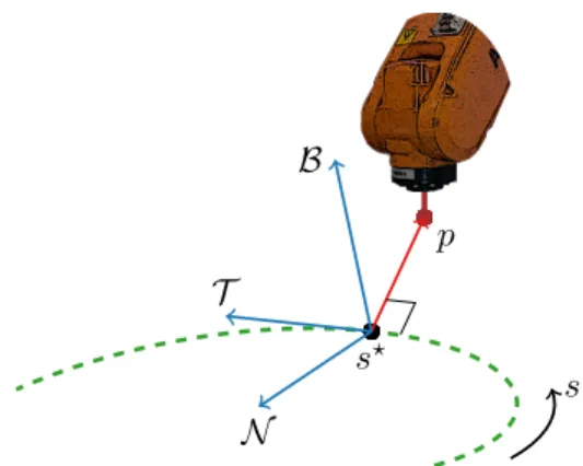
−σN. (3) Furthermore, let p(t) be the vector of positional coordi-nates at fixed time t in the inertial world frame (forward position kinematics of the robotic manipulator), then the point on the path γclosest top(t)isγ(s?), where
r(s, t) =p(t)−γ(s) (4) s?= arg min s 1 2kr(s, t)k 2 2. (5)
See Fig. 1 for an illustration of the concept.
As is clear from (4)-(5), finding s?(t) involves an
opti-mization problem. Since it is undesired to embed this into a higher-level optimization problem, we attempt to find the temporal evolution of s?(t) by looking at the optimality
s
s
?p
T
N
B
Fig. 1: Illustration of the position of the end-effector with respect to the closest position of the path.
conditions. Recall that for unconstrained optimization, the necessary first order optimality condition is:
0 = d ds 1 2kr(s, t)k 2 2 (6a) =r(s, t)Tγ0(s). (6b)
Consider that the position s? is known at an initial
time-point, we can enforce the solution to be optimal in time by setting the time derivative of the necessary first order optimality condition (6) to zero, i.e.,
0 = d dt
r(s, t)Tγ0(s) (7a)
= (v(t)−γ0(s) ˙s(t))Tγ0(s) +r(s, t)Tγ00(s), (7b)
wherev(t) =dpd(tt). This ultimately gives us a closed formula for the velocity of the point on the path closest top(t),
˙
s(t) = v(t)
TT (s)
1−κ(s)r(s, t)TN(s). (8)
B. Spatial reformulation
To facilitate the time-transormation, the robot dynamics are augmented with r = [rx, ry, rz]. Additionally, the state
t(s)is included to keep track of the evolution of time. The state vector then reads ξ= [q,q, r, t˙ ]. Using the established representation for the dynamics of the position of the end-effector p(t) with respect to the path, we perform a spatial transformation of the equations of motion:
ξ0 :=dξ ds = dξ dt dt ds, (9) with the state vectorξ. Fors˙(t)6= 0, we have thatddts= s˙(1t), and therefore ξ0 = 1 ˙ s(t) ˙ ξ. (10)
The resulting equations of motion are: dq ds = ˙ q ˙ s (11a) M(q)d ˙q ds = τ−C(q,q˙) ˙q−G(q) ˙ s (11b) dr ds = ˙ p ˙ s −T(s) (11c) dt ds = 1 ˙ s, (11d) (11e) where the velocity of the end-effector can be written as
˙
p=J(q) ˙q, withJ(q)the robot Jacobian, ands˙ is obtained from (8).
The time transformation applied above is highly nonlinear, but is nevertheless appealing for two reasons. First, with the newly obtained state variable t(s) and the according first-order differential equation dt
ds, time-optimal motion is
equivalent to minimizingt over the motion along the path. Secondly, the required knowledge about the temporal evolu-tion of theT,N andBvectors describing the local Frenet-Serret frame and many other geometric properties (such as obstacles) at time t become explicitly available in the integration scheme forξ0.
III. OPTIMAL CONTROL PROBLEM FORMULATION
In order to illustrate the benefits of the spatial reformula-tion of the robot dynamics, we formulate a time-optmimal trajectory generation problem. The OCP we intend to solve is stated as minimize ξ(·)∈Rnx, τ(·)∈Rm tf= Z tf t=0 dt (12a) subject to ξ˙(t) =f(ξ(t), τ(t)) ∀t∈[0, tf] (12b) g(p(t))≤0 ∀t∈[0, tf] (12c) τ(t)≤τ(t)≤τ(t) ∀t∈[0, tf] (12d)
with system dynamics, path constraints and torque bounds as constraints, respectively. This formulation is not readily passed to an optimization routine, as the time interval[0, tf]
on which we solve the OCP is not independent of the optimization variables. Therefore, we proceed to pose two reformulations of the above OCP, which we will compare in the subsequent sections. The first is a time-optimal formu-lation using a rescaling of the time variable, with geometric constraints as nonlinear constraints. The second one makes use of our proposed spatial reformulation.
For both formulations,ξ= [q,q, r, t˙ ]T is the state vector
andτ are the controls.
A. Time-scaled time-optimal control problem
We introduce θ =t/tf as a scaling of the time variable.
Furthermore, for the formulation in time, we do not make use of a predefined path, so we take γ(s) = 0; this results inr=p. In this way, notation is consistent with the spatial
formulation. Using a linear time scaling as described above, the OCP in (12) becomes
minimize ξ(·)∈Rnx, τ(·)∈Rm tf= Z 1 θ=0 tfdθ (13a) subject to dξ(θ) dθ =tf·f(ξ(θ), τ(θ)) ∀θ∈[0,1] (13b) gθ(r(θ))≤0 ∀θ∈[0,1] (13c) τ(θ)≤τ(θ)≤τ(θ) ∀t∈[0,1] (13d) Using the above linear rescaling, we are indeed capable of making the time interval [0, tf] = [0,1] independent of the
decision variablesξ, τ.
B. Spatial time-optimal control problem
From (10), we can get the spatial dynamics as f(ξ(s), τ(s))/s˙. The optimal control formulation then reads as minimize ξ(·)∈Rnx, τ(·)∈Rm tf= Z sf s=0 dt dsds (14a) subject to ξ0(s) =f(ξ(s), τ(s)) ˙ s ∀s∈[0, sf] (14b) gs(r(s))≤0 ∀s∈[0, sf] (14c) τ(s)≤τ(s)≤τ(s) ∀s∈[0, sf] (14d)
where we obtains˙ from (8).
Note that both OCPs (13) and (14) are equivalent to (12), as the objective function and the constraints remain equivalent after transformation of variables.
IV. NUMERICAL ALGORITHMS
To numerically solve the optimal control problems of the previous section, we adopt the open-source CasADi [3] software framework, which has been proven to solve OCPs reliably and efficiently [5]. More specifically, we use the Python front-end to formulate the OCP as a nonlinear program (NLP) using Bock’s multiple shooting method [7] as a discretization method. To this end, we relied on the integratorscvodesandidasinside the sundials suite [1]. The resulting NLP is passed to the open-source solver IPOPT [20]. It implements a primal-dual interior point method suited for solving large-scale NLPs. The linear algebra subroutine calls were passed to the sparse solver
ma57from the HSL library [2]. Note that all of the software packages mentioned above can be conveniently called from within the CasADi framework.
For the second part of the simulations, we use a 6-DOF robot model, which is constructed with the Python-based toolbox SympyBotics [15].
V. SIMULATION RESULTS
We show the performance of our time-optimal OCP with spatial reformulation of the dynamics on a simple three link robot manipulator of which the Denavit-Hartenberg parameters are shown in Table I. We consider two different
TABLE I: Denavit-Hartenberg parameters for the three-link robot used in simulation
d[m] θ[rad] a[m] α[rad]
Link 1 0.1 0 0 π/2
Link 2 0 π/2 1 0 Link 3 0 −π/2 0.7 0
motion experiments: the first is a time-optimal point-to-point motion, where we compare the results of both the spatial reformulation and the linear time scaling. The second is a problem where no end effector position is specified, and we introduce a static obstacle.
Note that in the following, a small control regularization of the formrτPiτi2, withrτ = 10−4is added to the objective
function in order to obtain smooth control trajectories. A. Time-optimal point-to-point motion
To illustrate the equivalence of both methods discussed in Section III, we solve the OCPs (13)-(14) for a simple time-optimal motion planning task. The robot end-effector travels from a starting pointp0 to a fixed final positionpf,
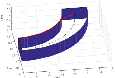
staying inside a certain space, defined as the space between two cilinders, see Fig. 2.
This constraint might be posed for the time-dependent formulation as
R≤ k[rx(θ), ry(θ)]k2≤R, ∀θ∈[0,1], (15a)
Z≤rz(θ)≤Z, ∀θ∈[0,1]. (15b)
Recall that, for the time-domain formulation, r denotes the vector from the origin to the end-effector. For the spatial formulation the constraints read as
Rs≤rTN(s)≤Rs, ∀s∈[0, π/2], (16a) Z ≤rz(θ)≤Z, ∀s∈[0, π/2], (16b) with T(s) = [−sin(s),cos(s),0]T, N(s) = [−cos(s),−sin(s),0]T, B(s) = [0,0,1]T, κ= 1.0 m−1, σ= 0.0 m−1.
The graph in Fig. 2 corresponds with the values R = 0.8 m,R = 1.2 m, Rs= 0.2 m,Rs= 0.2 m,Z =−0.1 m,
Z= 0.1 m.
One advantage of the spatial reformulation follows from the comparison of (16a) and (15a): in the latter case, the path constraint is convex, in the first it is not. If the convexity holds for the constraint functions, convergence of the NLP solver is often accelerated.
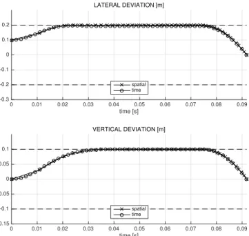
We compare the solution of the two different formulations in Fig. 3. The solution trajectories of both methods are shown as a function of time. The torque trajectories clearly show that the methods result in different discretizations. The spatial formulation yields a solution that takes longer time-steps in
1.4 1.2 1 0.8 0.6 Y [m] 0.4 0.2 0 1.4 1.2 1 0.8 0.6 X [m] 0.4 -0.2 -0.1 0 0.2 0.1 0.2 0 Z [m]
Fig. 2: Time-optimal solution (red) of optimal control prob-lems (13) and (14) with cylindrical path constraints. The con-straint space is delimited with dark blue faces, the centerline is shown in black.
the beginning of the interval than the time-based formulation, which takes equidistant steps. It is clear from the figure that the resulting trajectories for the lateral and vertical deviation from the centerline of the cylindrical path are the same, up to the different discretizations. For a finer discretization grid, these differences vanish.
Another interesting remark is that the constraint on the first joint torque is active throughout the entire interval, as we would expect in a time-optimal motion. In addition, the path constraints are seen to be active most of the times as well, except to meet the initial and end point constraints. To conclude the comparison, we examine the NLP solver convergence. In this particular example, the time-optimal OCP was solved faster with the spatial formulation than the time formulation: the interior point solver needed 35 iterations (1.703 s) instead of 43 (1.753 s). More experiments need to be carried out to confirm this as a general rule. B. Time-optimal obstacle avoidance
A major advantage of employing the time transformation instead of the conventional formulation, is the natural way to insert geometric constraints. Also, this method is suited for arbitrary paths in space, not just analytical ones as in the above example. Both properties are made apparent in the following simulation result, where we consider a 6-DOF ABB IRB120 industrial robot (Fig. 4) [4]. The simulation experiments are based on a dynamic model of this robot that was made available by ABB, albeit without taking friction into account.
In the following example, we perform a time-optimal motion planning task. The robot has to follow a given path within given tolerances as fast as possible, avoiding a static cylindrical obstacle at the end of the path. Additionally, we constrain the end-effector to point vertically down by imposing additional constraints on the forward orientation kinematics. The path specified (cf. dotted line in Fig. 5) is a planar path with piecewise constant curvature and given
time [s] 0 0.01 0.02 0.03 0.04 0.05 0.06 0.07 0.08 0.09 -0.3 -0.2 -0.1 0 0.1 0.2 LATERAL DEVIATION [m] spatial time time [s] 0 0.01 0.02 0.03 0.04 0.05 0.06 0.07 0.08 0.09 -0.15 -0.1 -0.05 0 0.05 0.1 VERTICAL DEVIATION [m] spatial time
(a) The lateral and vertical deviation are taken with respect to the centerline between the two cilinders.
time [s] 0 0.01 0.02 0.03 0.04 0.05 0.06 0.07 0.08 0.09 -1000 -500 0 500 1000 JOINT 1 TORQUE [Nm] spatial time time [s] 0 0.01 0.02 0.03 0.04 0.05 0.06 0.07 0.08 0.09 -1000 -500 0 500 1000 JOINT 2 TORQUE [Nm] spatial time time [s] 0 0.01 0.02 0.03 0.04 0.05 0.06 0.07 0.08 0.09 -1000 -500 0 500 1000 JOINT 3 TORQUE [Nm] spatial time
(b) The torques in the robot joints.
Fig. 3: Comparison of the solution of the two OCP formu-lations (13) and (14). The joint torque bounds are taken to be−1000 Nm≤τ≤1000 Nmfor both formulations.
Fig. 4: Sketch of the ABB IRB120 industrial robot. During the simulation, the end-effector points down (as shown).
initial tangent and normal vectors, both normalized. The binormal, which is vertical at all points, is taken arbitrarily as B0 = [0,0,1]. The cartesian coordinates of the path can
be retrieved by integrating the Frenet-Serret formulas (3) forward in the path coordinate s, starting at s0 = 0 m.
Note that this integration can be incorporated in the state equations (which are already in function ofs) by augmenting the dynamics with (3).
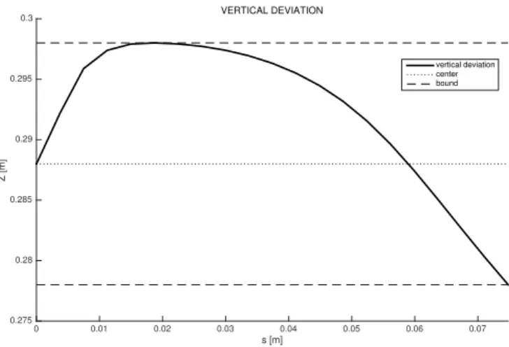
At the end of the prespecified path, there is a static cylin-drical obstacle narrowing down the maneuvering possibilities of the end-effector. In the spatial formulation, this constraint will amount to increasing the lower bound of the constraint 16a; it remains a simple bound. The resulting time-optimal path can be seen in Fig. 5. Again, we see that the path touches the inner path constraint as we expect for time-optimal trajectories. Note that in this case, the final position of the end effector is not completely specified, only constrained to lie in the plane spanned byN andB. The vertical deviation is depicted in Fig. 6. Also here the constraints on the vertical deviation become active at some point in the motion. At the end of the interval, the robot ”falls down”, i.e. it is using gravity in order to save time.
Note that the time-domain formulation (13) is not readily applicable in this example, because the path constraints are not straightforward to compute in the time domain for arbitrary paths, in contrast with paths with an analytical de-scription, as in the first example. This shortcoming originates from the fact that we do not know on beforehand where in the configuration space the end effector will be at which point in time, i.e. the relation betweentandsis not stated explicitly. An expression of the path constraints in the time domain results in possibly very nonlinear constraints; this holds even more so for static obstacles as in the above example.
VI. CONCLUSION
In this paper, we introduced a path-parametric system reformulation for robotic manipulators. It is aimed at conve-nience for path specification, and exhibits a natural way to impose geometric constraints. These advantages have been shown in relation to optimal control using a time-scaling approach, which does not posess these properties.
X [m] 0.54 0.55 0.56 0.57 0.58 0.59 0.6 Y [m ] -0.07 -0.06 -0.05 -0.04 -0.03 -0.02 -0.01 0
0.01 TIME-OPTIMAL PATH WITH OBSTACLE AVOIDANCE
end effector path center path constraint
Fig. 5: Top view of the time-optimal path around an arbitrary central path with piecewise constant curvature. At the end of the path, there is a static obstacle narrowing the available space of the robot end-effector.
s [m] 0 0.01 0.02 0.03 0.04 0.05 0.06 0.07 Z [m] 0.275 0.28 0.285 0.29 0.295 0.3 VERTICAL DEVIATION vertical deviation center bound
Fig. 6: Vertical deviation from the z = 0.288 m horizontal plane for the time-optimal optimal control problem with obstacle avoidance.
The work presented here forms the groundwork for future developments. A first follow-up of the results showed is to assess the novel method on an experimental testbed. Joint and control trajectories can be computed offline, in a similar fashion as to compute the simulation results showed. To this end, an effective way of taking into account Coulomb and viscous friction is needed.
Another possible advancement lies in the application of the presented techniques in a model predictive framework, both in simulation and on a real-life robot setup. More specifically, the application of this method in real-time seems a computational challenge, although the first steps in this
direction have been taken. Lastly, a setup running entirely online, where path information is not specified in advance but, for instance, supplied by human interaction via a manual control device could exploit all the computational advantages proposed above to a greater extent.
REFERENCES
[1] Sundials - SUite of Nonlinear and DIfferen-tial/ALgebraic equation Solvers (web page and software). https://computation.llnl.gov/casc/sundials, 2009.
[2] Hsl(2011). a collection of fortran codes for large scale scientific computation. http://www.hsl.rl.ac.uk, 2011.
[3] CasADi. http://casadi.org, 2013. [Online; accessed 10-October-2013].
[4] ABB. IRB120 technical data, 2015. [Online (http://new.abb.com/products/robotics); accessed 22 September 2015].
[5] J. Andersson, J. ˚Akesson, and M. Diehl. CasADi – A symbolic package for automatic differentiation and optimal control. In S. Forth, P. Hovland, E. Phipps, J. Utke, and A. Walther, editors,Recent Ad-vances in Algorithmic Differentiation, Lecture Notes in Computational Science and Engineering, Berlin, 2012. Springer.
[6] J.E. Bobrow, Steven Dubowsky, and J.S. Gibson. Time-optimal control of robotic manipulators along specified paths. The International Journal of Robotics Research, 4(3):3–17, September 1985.
[7] H.G. Bock and K.J. Plitt. A multiple shooting algorithm for direct solution of optimal control problems. InProceedings 9th IFAC World Congress Budapest, pages 242–247. Pergamon Press, 1984. [8] F. Debrouwere, Van Loock W., G. Pipeleers, and J. Swevers.
Time-optimal tube following for robotic manipulators. In2014 IEEE 13th International Workshop on Advanced Motion Control (AMC), 2014. [9] T. Faulwasser, B. Kern, and R. Findeisen. Model predictive
path-following for constrained nonlinear systems. In Joint 48th IEEE conference on Decision and Control and 28th Chinese Control Con-ference, 2009.
[10] J. V. Frasch, A. J. Gray, M. Zanon, H. J. Ferreau, S. Sager, F. Borrelli, and M. Diehl. An Auto-generated Nonlinear MPC Algorithm for Real-Time Obstacle Avoidance of Ground Vehicles. InProceedings of the European Control Conference, 2013.
[11] Y. Gao, A. Gray, J. V. Frasch, T. Lin, E. Tseng, J.K. Hedrick, and F. Borrelli. Spatial predictive control for agile semi-autonomous ground vehicles. InProceedings of the 11th International Symposium on Advanced Vehicle Control, 2012.
[12] Heinrich Guggenheimer.Differential Geometry. Dover, 1977. [13] D. Lam, C. Manzie, and M. Good. Model Predictive Contouring
Control. In469th IEEE Conference on Decision and Control, 2010. [14] Kang G Shin and Neil D McKay. Minimum-time control of robotic
manipulators with geometric path constraints. IEEE Transactions on Automatic Control, 30(6):531–541, June 1985.
[15] Cristvo Duarte Sousa. Sympybotics v1.0, August 2014.
[16] Mark W Spong, Seth Hutchinson, and Vidyasagar. Mathukumalli.
Robot modeling and control, volume 3. Wiley, 2006.
[17] Niels van Duijkeren, Tamas Keviczky, Peter Nilsson, and Leo Laine. Real-Time NMPC for Semi-Automated Highway Driving of Long Heavy Vehicle Combinations. In proceedings of the 5th IFAC Conference on Nonlinear Model Predictive Control 2015 (NMPC’15), Sevilla, Spain, 2015.
[18] D. Verscheure, B. Demeulenaere, J. Swevers, J. De Schutter, and M. Diehl. Time-Optimal Path Tracking for Robots: a Convex Optimization Approach. IEEE Transactions on Automatic Control, 54:2318–2327, 2009.
[19] R. Verschueren, S. De Bruyne, M. Zanon, J. V. Frasch, and M. Diehl. Towards Time-Optimal Race Car Driving using Nonlinear MPC in Real-Time. InProceedings of the 53rd Conference on Decision and Control (CDC), 2014.
[20] A. W¨achter and L.T. Biegler. On the Implementation of a Primal-Dual Interior Point Filter Line Search Algorithm for Large-Scale Nonlinear Programming.Mathematical Programming, 106(1):25–57, 2006.