MERCURY CONCENTRATIONS AND FEEDING ECOLOGY OF FISHES IN ALASKA
By
Andrew Philip Cyr, B.S.
A Dissertation Submitted in Partial Fulfillment of the Requirements for the Degree of Doctor of Philosophy
In Fisheries
University of Alaska Fairbanks May 2019
Andrew P. Cyr
APPROVED:
Dr. Juan Andres López, Committee Chair Dr. Todd O'Hara, Committee Member Dr. Matthew Wooller, Committee Member Dr. Andrew Seitz, Committee Member
Dr. Milo Adkison, Chair Department of Fisheries
Dr. Bradley Moran, Dean College of Fisheries and Ocean Sciences
Dr. Michael Castellini Dean of the Graduate School
Abstract
Mercury (Hg) is a ubiquitous contaminant found in nearly every fish species analyzed. Certain forms of Hg accumulate efficiently in fish tissues, sometimes reaching concentrations of concern for human and wildlife health when consumed. This has motivated considerable research and interventions surrounding fish consumption with Hg concentrations as the underlying cause of over 80% of fish consumption advisories in the United States and Canada. The ecological and physiological drivers that influence the concentrations of Hg in fishes are complex and vary among taxa spatially and temporally. Studying these drivers and their respective influences on Hg concentrations can help elucidate observed differences in Hg concentrations across space and time, which can then be used to improve management and consumption strategies. Here I present a series of studies focused on the chemical feeding ecology of Hg by measuring total Hg (THg) concentrations and ratios of nitrogen and carbon stable isotopes in multiple fish species from three regions in Alaska. In Chapter 2 I described foundational field collection efforts to characterize the fish communities from West Creek and the Taiya River in Klondike Gold Rush National Historical Park, and the Indian River in Sitka Historical National Park, Alaska. This chapter and agency report presents a survey of the fish species assemblage of the rivers and laid the framework for the regional analyses I conducted in the study presented in Chapter 3. In Chapter 3 I report inter- and intra river comparisons of THg concentrations and associated feeding ecology of riparian Dolly Varden, separated by anadromous barriers in each system. I concluded that resident Dolly Varden that co-habit riverine locations with spawning salmon consume more salmon eggs than resident Dolly Varden from other locations of the same river that do not co-habit with spawning salmon. This is reflected in the isotopic composition of their tissues, and subsequently the THg concentrations of these fish are lower relative to Dolly Varden from parts of the same river above anadromous barriers. In Chapter 4, I describe regional patterns of THg concentrations and stable isotope values of carbon and nitrogen in nine species of fish and invertebrates from the Bering Sea and North Pacific Ocean along the Aleutian Islands, using Steller sea lion management zones as a spatial framework. I determine that most species from the Western Aleutian Islands have greater THg concentrations, and more negative δ13C values than those from the
Central Aleutian Islands, indicating ecosystem-wide differences in THg concentrations and fish feeding ecology. I also determined that Amchitka Pass, a well-documented oceanographic and ecological divide along the Aleutian Island chain, aligns better with differences in THg concentrations than the boundary between Steller sea lion management zones. In Chapter 5, I report THg and methylmercury
concentrations in fishes of Kotzebue Sound, including seven species that are important for subsistence users. I determined that fork length influences Hg concentrations within individual species, and that trophic relationships within a food web, a factor associated with biomagnification, influences Hg concentrations across the entire food web. I also observed that muscle tissues from virtually every individual fish had Hg loads below the State of Alaska's criteria for unlimited consumption. Taken together, the work conducted in this dissertation helps us better understand the ecological dynamics of Hg in aquatic food webs and has contributed to Hg monitoring of fish resources across parts of Alaska.
Acknowledgements
This dissertation would not have been possible without the tireless efforts and patience of my friends and colleagues. I would like to thank my committee for all their assistance, patience and guidance at every step of the process. Similarly, I would like to thank my coauthors for their valuable insight and guidance on each step of each manuscript. Todd O'Hara and J. Andres López were enormously helpful through all aspects of my research, and continually provided me with new and exciting opportunities to expand my skill sets and professional development. Collectively, the support of all those behind the scenes helped keep me focused and to take charge of my research to make the difficult decisions at the right moments.
I would like to thank the Wildlife Toxicology Lab community for their assistance. To my fellow graduate students John Harley, Stephanie Kennedy, Marianne Lian, and Stephanie Crawford for all their help corralling me and keeping me moving forward despite my frustrations, limitations, and self-imposed restrictions. Similarly, I would like to thank the many undergraduate students that assisted me throughout the laboratory portion of my research. The many hours of work they contributed are the only reason the immense amount of lab work required for this project was ever completed. A well-deserved thank you to Maggie Castellini for keeping the lab running despite the chaos I brought to it, and my ability to break things and make her blood boil. It goes without saying that none of this would have been possible without her hard work, guidance, knowledge, and of course her patience. I would also like to thank Cathy Griseto for being the ever-present smart ass to keep things in perspective and helping me with all manner of paperwork, logistics, and staying on track in general.
None of the research presented here would have been even remotely possible without the generous support of numerous funding groups and agencies. I would like to thank the National Park Service, the Alaska Department of Environmental Conservation, the North Pacific Research Board (NPRB), Biomedical Learning and Student Training (BLaST), and the Graduate School for a Thesis Completion Fellowship, all of which contributed funding for various portions of my research and degree.
In particular, I would like to thank the BLaST program. Not only did they fund a significant portion of my research, they also provided me with more opportunities for mentoring, outreach, conferences and
trainings than most graduate students ever receive. The support of the BLaST program and staff has been instrumental in assisting me throughout my research and guiding my interests both throughout graduate school, as well as into the future.
A collective thank you to the many friends, family, coworkers, and random other people that encouraged me in some capacity to pursue a graduate degree in this research field. This includes Anna Bryan, Bobbie Sandwich, Erin Gleason, Aaron Wells, Brian Jackson, J.J. Frost, Adrian Gall, and countless others that I have forgotten to mention here.
Finally, I would like to thank my friends and family. My parents and sister might not have a clue what I do (don't worry, neither do I!), but they have supported me and encouraged me every step of the way. And I promise you Mom and Dad, I will get a real job sometime, maybe even after I finish this degree. Maybe... Finally, I would like to thank my girlfriend Stephanie Kennedy who has miraculously maintained composure and patience with me while I struggled and couldn't find the traction and confidence to move forward. Thank you.
Table of Contents
Page
Abstract...iii
Acknowledgements ... v
List of Figures... xiii
List of Tables ... ... xv
Chapter 1 - Introduction ... 1
1.1 Introduction...2
1.2 Mercury Exposure... 2
1.3 Linking Humans and Fish Together... 3
1.4 A Notable Human Dietary Exposure Example ... 3
1.5 Ecological Research Tools for Examining Food Webs ... 4
1.6 Organization of Dissertation ... 6
1.7 Works Cited ... 8
Chapter 2 - Developing a freshwater contaminants monitoring protocol for the Southeast Alaska Network ... 13
2.1 Abstract ... 14
2.2 Introduction...15
2.3 Methods... 16
2.3.1 River description and selection ... 16
2.3.1.1 Klondike Gold Rush National Historical Park ... 16
2.3.1.1.1 Taiya River... 16
2.3.1.1.2 Nourse River ... 17
2.3.1.1.3 West Creek ... 17
2.3.1.2 Sitka National Historical Park... 17
2.3.1.2.1 Indian River... 17
2.3.2 Fish species selected ... 18
2.3.3 Permits, animal care and use authorizations ... 18
2.3.4 Sample site selection ... 18
2.3.5 Trapping and fish handling ... 19
2.4 Results ... 20
2.4.1 Klondike Gold Rush National Historical Park ... 20
2.4.1.1 Taiya River... 20
2.4.1.2 Nourse River ... 21
2.4.1.3 West Creek ... 21
2.4.1.4 KLGO sampling summary ... 22
2.4.2 Sitka Historical National Park...23
2.4.2.1 SITK sampling summary ... 24
2.5 Discussion ... 24
2.6 Next steps ... 25
2.7 Figures... 27
2.8 Tables ... 31
2.9 Works Cited ... 37
Chapter 3 - Assessing the influence of migration barriers and feeding ecology on total mercury concentrations in Dolly Varden (Salvelinus malma) from a glaciated and non-glaciated stream 39 3.1 Abstract ... 40
3.2 Introduction...41
3.3 Methods... 44
3.3.1 Study sites and fish sampling. ... 44
3.3.2 Fish tissue preparation ... 45
3.3.3 Total mercury (THg) analysis ... 46
3.3.4 Carbon and nitrogen stable isotope analysis ... 46
3.3.5 DV otolith estimation ... 47
3.3.6 Statistical analysis ... 48
3.4 Results ... 49
3.4.1 Descriptive overview ... 49
3.4.2 Modeling [THg] using Dolly Varden length, watershed characteristics, δ15N, and δ13C... 50
3.4.3 Mean [THg] by fish and watershed characteristics ... 50
3.4.4 [THg] in relation to C and N stable isotope values ... 51
3.4.5 Carbon and nitrogen isotope relationships ... 51
3.4.6 Spawning pink salmon contribution of THg to each river ... 52
3.5 Discussion ... 52 3.6 Conclusions ... 57 3.7 Acknowledgments... 57 3.8 Figures... 58 3.9 Tables ... 62 3.10 Appendices... 64
3.11 Works Cited ... 67
Chapter 4 - Mercury concentrations in marine species from the Aleutian Islands: spatial and biological determinants ... 79 4.1 Abstract ... 80 4.2 Funding Sources... 81 4.3 Introduction...82 4.4 Methods... 84 4.4.1 Sampling ... 84 4.4.2 Sample processing ... 85 4.4.3 Total Hg analysis ... 85
4.4.4 Stable carbon and nitrogen isotope analysis ... 86
4.4.5 Lipid extraction and correction ... 86
4.4.6 Length standardization of [THg]... 87 4.4.7 Statistical analysis ... 88 4.5 Results ... 89 4.5.1 Data summary ... 89 4.5.2 Stable isotopes ... 89 4.5.3 Regional comparisons ... 90
4.5.4 [THg] in relation to trophic position ... 91
4.6 Discussion ... 92
4.6.1 Overview... 92
4.6.2 Isotopes and feeding ecology ... 92
4.6.3 Geographic trends ... 94
4.6.4 Yellow Irish lord ... 95
4.6.5 Food web dietary exposure ... 96
4.7 Conclusion ... 97 4.8 Acknowledgements... 98 4.9 Figures... 99 4.10 Tables ... 103 4.11 Appendices... 106 4.12 Works Cited ... 111
Chapter 5 - Mercury concentrations in subsistence fish from Kotzebue Sound, Alaska: Community-based effort to understand drivers and public health ... 121
5.1 Abstract ... 122
5.2 Introduction... 123
5.3 Methods... 125
5.3.1 Study location and fish sampling ... 125
5.3.2 Fish processing... 126
5.3.3 Total Hg concentration ([THg]) analysis ... 126
5.3.4 Monomethylmercury concentration ([MeHg+]) analysis ... 127
5.3.5 Carbon and nitrogen stable isotope analysis ... 127
5.3.6 Lipid correction... 128
5.3.7 Sheefish otolith age estimation ... 128
5.3.8 Statistical analysis ... 129
5.4 Results... 130
5.4.1 Summary Results ... 130
5.4.2 Relationship of [THg] with fork length, δ15N values, and lipid-corrected δ13C values ... 131
5.4.3 [MeHg+] and %MeHg+ regression relationships with fork length, δ15N and lipid-corrected δ13C values ... 131
5.4.4 Modeling [THg], fork length, δ15N values, and lipid-corrected δ15C values...132
5.4.5 Sheefish age estimate relationships... 132
5.4.6 [THg] comparisons with State of Alaska fish consumption criteria ... 132
5.5 Discussion ... 133
5.5.1 SOA fish consumption comparisons ... 133
5.5.2 Ecological drivers of mercury concentration ... 133
5.5.3 MeHg+ ... 135 5.5.4 Case studies...136 5.5.5 Sheefish... 136 5.6 Conclusion ...136 5.7 Acknowledgments...137 5.8 Figures...138 5.9 Tables ...143 5.10 Works Cited ...146 Chapter 6 - Conclusions ... 157 6.1 Overview...158 6.2 Region ...158 6.3 Feeding ecology ...159
6.4 Fish resource Hg monitoring... 159
6.5 Fish [Hg] in context of other events and research... 160
6.6 Next steps... 162
6.7 Works cited ... 164
List of Figures
Page
Figure 2.1 - Photos demonstrating sample collection techniques using ultra-clean foil and nitrile
gloves...27
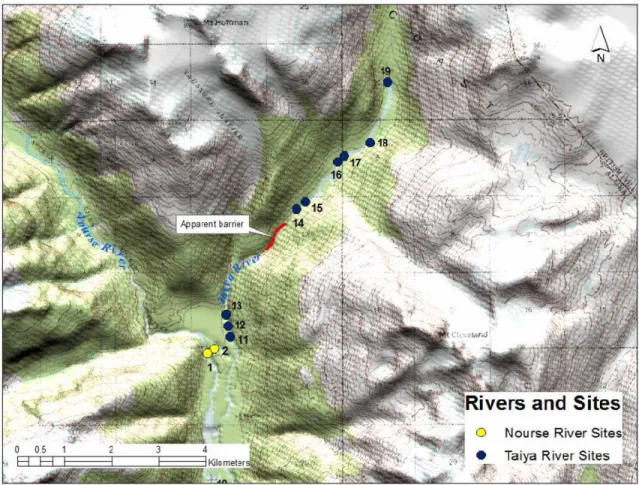
Figure 2.2 - Upper watershed sampling sites in KLGO, including Taiya (blue dots) and Nourse
(yellow dots) Rivers. ... 28
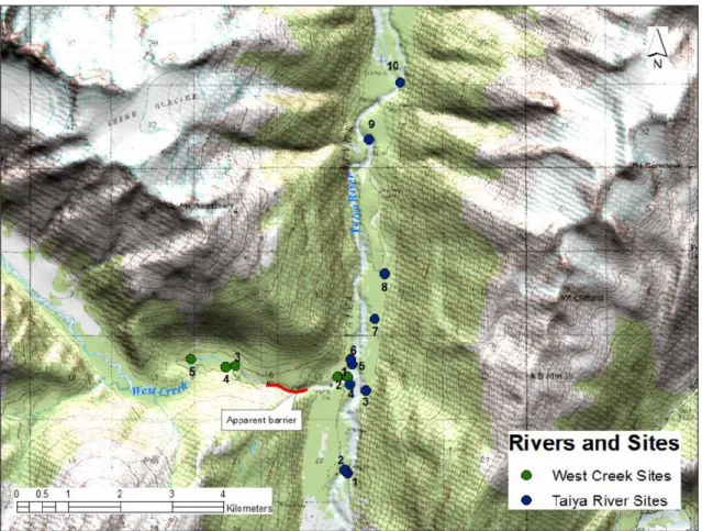
Figure 2.3 - Lower watershed sampling sites in KLGO, including Taiya River (blue dots) and West Creek (green dots). ... 29
Figure 2.4 - Representative photos of riverine habitat in KLGO (West Creek: left picture-above apparent barrier; right picture-below apparent barrier). Note the proximity of the glaciers to the study site, the density of the riparian vegetation, and the glacial silt color of the water. ... 30
Figure 2.5 - Sampling site locations in Indian River (SITK). ... 30
Figure 3.1 - Dolly Varden sampling reaches for West Creek and the Indian River. To maximize clarity, watersheds are not scaled relative to one another. Red rectangles represent apparent barriers to anadromous migration. Green boxes represent sampling reaches above and below barriers. Dark grey polygons represent glacier extent within the West Creek watershed... 58
Figure 3.2 - Unadjusted THg concentrations across all sampling sites generally increase with Dolly Varden fork length (linear regression; r2 = 0.27, P << 0.001). [THg] = Total mercury concentration...59
Figure 3.3 - Unadjusted THg concentrations (ng/g ww) and δ15N (‰) for individual fish from Indian River and West Creek, categorized by above and below anadromous barriers. THg = Total mercury... 60
Figure 3.4 - δ15N (‰) and δ13C (‰) stable isotopic space for individual fish from the Indian River and West Creek, categorized by above and below anadromous barriers... 61
Supplementary Figure 3.1 - Relationship between mass and fork length for all Dolly Varden
collected across all sampling sites. ... 66
Figure 4.1 - Map depicting the approximate extent of sample collection, within the context of Steller sea lion management regions. WAI is Western Aleutian Islands, and CAI is Central Aleutian Islands. ... 99
Figure 4.2 - Mean δ15N and lipid-corrected δ13C values (± 1 standard deviation) of muscle samples for each fish and invertebrate species, categorized by western Aleutian Islands (WAI) and central Aleutian Islands (CAI). VPDB is the isotopic standard Vienna Pee-Dee Belemnite, AIR is the isotopic standard atmospheric air... 100
Figure 4.3 - Box and whisker plot representing the length-standardized muscle [THg] for each fish and invertebrate species, characterized by region. Data presented on a log scale on the y-axis. Bold
horizontal lines inside each box represent median values, bottom and top edges of boxes represent 25th and 75th percentiles, respectively, and the ends of the vertical solid lines represent ± 1.5 * interquartile range. Length-standardized [THg] beyond this range are displayed as individual points. * denotes significance level between regions for the species indicated, α ≤ 0.01; **, denotes significance α ≤ 0.001. WAI is Western Aleutian Islands, and CAI is Central Aleutian Islands. ...101
Figure 4.4 - [THg] and δ15N values for muscle samples, individual species' regression slopes. WAI is Western Aleutian Islands, and CAI is Central Aleutian Islands. AIR is the isotopic standard
atmospheric air... 102
Supplementary Figure 4.1 - The difference between bulk and lipid-extracted δ13C values (Δ13C) and C:NBulk for all 245 samples. ...108
Supplementary Figure 4.2 - The difference between bulk and lipid-extracted δ13C values (Δ13C) and C:NBulk for samples with C:NBulk < 10. ...109
Supplementary Figure 4.3 - δ Clipid-extracted values and δ13Clipid -corrected values, derived using the mathematical correction formula: δ13CLipid-corrected = δ13CBulk -1.48 + (0.65 * C:NBulk). Data is restricted to C:NBulk < 10. Red dashed line is the y = x line. ... 110
Figure 5.1 - Regional map depicting study area...138
Figure 5.2 - Muscle total mercury concentrations [THg] and fork length (cm) of fishes from Kotzebue, Alaska. Absence of regression line indicates the relationship for that species was not
significantly different from zero.. ... 139
Figure 5.3A and 5.3B - Box and whisker plots of muscle total mercury concentrations [THg], methylmercury+ concentrations (MeHg+], and δ15N (‰) values for each fish species from Kotzebue, Alaska. Bold horizontal lines inside each box represent median values, bottom and top edges of boxes represent 25th and 75th percentiles, respectively, and the ends of the vertical solid lines represent ± 1.5 * interquartile range. Dashed line indicates the State of Alaska unrestricted consumption criteria (200 ng/g ww) for fish consumers. ww = wet weight. Letters a, b, and c indicate significant difference (a ≤ 0.05) for mean [THg] or mean [MeHg+] between species. δ15N values compared to the isotopic
standard air... 140
Figure 5.4 - %MeHg and δ15N (‰) values for each species of fish from Kotzebue, Alaska. Dashed line indicates %MeHg = 100%. δ15N values compared to the isotopic standard air...141
Figure 5.5 - Mean δ15N (‰) and lipid-corrected δ13C (‰) isotopic values ± standard deviation of muscle samples for each species of fish from Kotzebue, Alaska. δ15N values compared to the isotopic standard air, and δ13C values compared to the isotopic standard Vienna-PeeDee Belemnite (VPDB). ... 141
Figure 5.6 - Linear regressions for sheefish muscle total mercury concentrations [THg] with age, and muscle δ15N (‰) values with age. δ15N values compared to the isotopic standard air. ww = wet
List of Tables
Page
Table 2.1 - Trapping effort, fish counts, and catch per unit effort (CPUE) at sample sites on the Taiya
River in KLGO (July 25 to August 2, 2013)... 31
Table 2.2 - Trapping effort, fish counts, and catch per unit effort (CPUE) at sample sites on the Nourse River in KLGO (July 31 to August 1, 2013)...32
Table 2.3 - Trapping effort, fish counts, and catch per unit effort (CPUE) at sample sites on West Creek in KLGO (July 25 to July 28, 2013)... 32
Table 2.4 - Site coordinates (WGS84) and descriptions for the Taiya River in KLGO... 33
Table 2.5 - Site coordinates (WGS84) and descriptions for the Nourse River in KLGO...34
Table 2.6 - Site coordinates (WGS84) and descriptions for West Creek in KLGO... 34
Table 2.7 - Trapping effort, species counts, and catch per unit effort (CPUE) at sample sites on the Indian River in SITK (August 14 to August 17, 2013)... 35
Table 2.8 - Site coordinates (WGS84) and descriptions for the Indian River in SITK... 36
Table 3.1 - Morphometrics, age, mercury, and stable isotope values for Dolly Varden collected across sampling sites in West Creek and Indian River. Values are mean ± SD (note that both THg columns are reported as the geometric mean). N represents the total samples run for THg and stable isotope analysis. The numbers in parentheses represent how many samples out of N were smaller individuals pooled together to meet minimum tissue mass requirements (see Methods). [THg] = Total mercury concentration based on a ratio of girth to length as utilized by Rea et al. (2016)... 62
Table 3.2 - The best set of candidate models describing the relationship between total mercury concentrations in individual Dolly Varden and fish length, watershed characteristics, and δ15N composition. Length = individual fish length (mm); River = individual river system (West Creek or Indian River); Barrier = fish location relative to anadromous migration barrier (above or below)... 62
Table 3.3 - Parameter Akaike weighs (w+(j)) calculated from all candidate models describing the relationship between total mercury in individual Dolly Varden and fish length, watershed characteristics, and δ15N composition. Length = individual fish length (mm); River = individual river system (West Creek or Indian River); Barrier = fish location relative to anadromous migration barrier (above or below)...62
Table 3.4 - ANOVA test results of mean stable isotope values (N, δ15N (‰); and C, δ13C (‰)). * denotes a significance of P = 0.001, ** denotes a significance of P = 0.0001, no asterisk denotes no significance... 63
Supplementary Table 3.1 - Morphometrics and age for pooled samples of Dolly Varden collected across sampling sites in West Creek and Indian River. Values are mean ± SD. N represents the number of individual fish comprising the pooled sample...64
Supplementary Table 3.2 - The full candidate set of 32 multiple linear regression models evaluating the ability of five predictor variables (individual river system, fish location relative to anadromous migration barrier, fish length, δ15N, and lipid-corrected δ13C) to estimate unadjusted total mercury concentration in individual DV. Length = individual fish length (mm); River = individual river system (West Creek or Indian River); Barrier = fish location relative to anadromous migration barrier (above or below)...65
Table 4.1 - Total mercury concentrations ([THg]) and stable nitrogen and carbon isotope values for western Aleutian Islands (WAI) and central Aleutian Islands (CAI) fishes and cephalopods. Sample sizes (N) for each region, fork length (cm), mass (g), [THg] as measured (ng/g ww), length-
standardized [THg] in ng/g ww, δ15N values, bulk δ13C values, and lipid-corrected δ13C values for each species in the dataset. Data are means ± SD, geometric mean for [THg]...103
Table 4.2 - Differences in the lipid-corrected δ13C regional values (ΔCAI-WAI), and the regional difference (P values) for isotopic space comparisons for each species. Significance determined by
Hotelling's T2 test comparing mean δ15N and δ13C values in multivariate space... 104
Table 4.3 - Variance explained (R2) and significance (P value) for linear regression of unadjusted total mercury concentrations ([THg]) and δ15N values for western (WAI) and central (CAI) Aleutian
Islands... 104
Table 4.4 - Significance (P value) from general linear models of the influence of δ15N values, lipid- corrected δ13C values, the interaction of δ15N values and region, and the interaction of lipid-corrected δ13C values and region on unadjusted total mercury concentrations ([THg]) for each fish species...105
Supplemental Table 4.1 - Sample size, δ13CBulk values, δ13CLipid-extracted values, C:NBulk values, C:NLipid- extracted values, the difference in δ13C values between bulk and lipid-extracted (Δ13C), δ13CLipid-corrected values, and the difference in δ13C values between lipid-extracted and lipid-corrected (Δ13C). Lipid- corrected values are the δ13C values generated from the lipid-correction formula: δ13CLipid-corrected = δ13CBulk -1.48 + (0.68 * C:NBulk). Data restricted to samples with C:NBulk < 10... 106
Supplemental Table 4.2 - Summary statistics of sample size (N), fork length (cm), mass (g), total mercury concentration ([THg]) in ng/g ww, δ15N values, bulk δ13C values, and lipid-corrected δ13C values for all remaining western (WAI) and central (CAI) Aleutian Island fish and cephalopod species not included in statistical comparisons. Data are means ± SD, geometric mean for [THg]... 107
Supplemental Table 4.3 - Seasonal differences for lipid-corrected carbon (Δδ13C) and bulk nitrogen (Δδ15N) values for summer-winter for western (WAI) and central (CAI) Aleutian Islands. Significance determined by Hotelling's T2 test comparing mean δ15N and δ13C values in multivariate space... 108
Table 5.1 - Sample sizes (N), fork length, mass, muscle total mercury concentrations ([THg]), muscle monomethyl mercury concentrations ([MeHg+]), %MeHg+, δ15N values, δ13C values, and
lipid-corrected δ13C values for each fish species sampled near Kotzebue, Alaska. All data except %MeHg includes outliers, and is represented as mean ± SD. [THg] and [MeHg+] data are represented as geometric mean ± SD ng/g wet weight in the top cell, median and (range) in the bottom cell. %MeHg+ is displayed as the mean of individual values for each species in the top cell, and the slope of the
robust linear regression of [THg] and [MeHg+] in the bottom cell (Wagemann et al., 1997). ... 143
Table 5.2 - The amount of the linear regression variance explained (R2) and the significance (P value) for linear regression of total mercury concentrations ([THg]) with fork length, with δ15N values, and with the interaction of fork length and δ15N values for each species. Significant regressions in bold italic text. ... 144
Table 5.3 - The top four candidate models for approximating muscle [THg] within each species of fish in Kotzebue, Alaska, including fork length (cm), δ15N values, δ13C values, and the interaction of fork length and δ15N. The best candidate model for each species is highlighted in bold text. δ13C values are lipid-corrected δ13C values... 145
Chapter 1 - Introduction1
1Cyr, A.
1.1 Introduction
Mercury (Hg) is considered a “global contaminant” and consequently Hg contamination attracts worldwide attention, with particular interest on Hg contamination of aquatic organisms. The ecological and chemical processes underlying the Hg cycle enable efficient accumulation in aquatic food webs, particularly in the tissues of fish and top predators in fish-based ecosystems. As evidence of this, Hg has been detected in almost every fish species that has been measured from North America in the last several decades (AMAP 2011; Eagles-Smith et al. 2016). Due to the concentrations measured in some fish species, Hg is now responsible for over 80% of fish consumption advisories in the United States and Canada (Environment Canada, 2013; USEPA, 2011).
1.2 Mercury Exposure
Human and wildlife exposure to Hg is influenced by environmental chemistry, biochemistry and inter- and intra-species variation in feeding ecology. Hg is efficiently absorbed through the
gastrointestinal wall as the bioavailable form of monomethyl Hg (MeHg+), with an assimilation efficiency greater than 85% (Wang, 2012). The methylation of divalent Hg (Hg2+) to MeHg+ in the environment is highly variable and is influenced by environmental factors, notably the bacterial species present, water pH (Kelly et al., 2003), temperature (Johnson et al., 2016), ultraviolet light (Lehnherr and St. Louis, 2009), and the presence of dissolved cations or organic matter (Boening, 2000; Douglas et al., 2012). Fish also have limited capacity for redistributing, demethylating or eliminating total Hg (THg) or MeHg+, which leads to the variable accumulation and retention of THg or MeHg+ in muscle and other tissues (Amlund et al., 2007; Trudel and Rasmussen, 1997).
MeHg+ is a potent neurotoxin, involving oxidative stress and inhibiting selenium dependent enzymes (Farina et al., 2011; Ralston and Raymond, 2010). The ecotoxicological and biochemical properties of MeHg+ have led to considerable concern surrounding Hg exposure from dietary resources, and in particular the consumption of fish. A thorough understanding of the drivers of Hg accumulation in
the food web, and the importance of effective monitoring, is therefore vital for providing meaningful and targeted consumption advice.
1.3 Linking Humans and Fish Together
Fish are an especially important resource for many Alaskans. They represent a significant cultural connection for many Alaskans through family, history, and education (Barnhardt and Kawagley, 2005). Fish are also an important commercial resource for many communities in Alaska. Importantly, fish contribute significantly to the diet of many subsistence users in Alaska year-round. It is estimated that rural subsistence fishers in Alaska consume over 100 kg of fish annually (Fall, 2018; Robert J Wolfe, 2000). This level of consumption indicates a potential for significant dietary exposure to Hg. These details highlight the importance of understanding Hg concentrations ([Hg]) in Alaskan fish resources, and effective monitoring of the drivers that influence those [Hg] over time and space.
Because the Hg cycle is linked to the aquatic environment, dietary exposure to Hg is most prevalent through the consumption of contaminated fishes and aquatic invertebrates. However, dietary exposure to Hg is highly variable and dependent on numerous factors, such as species of fish, tissue type, fish age and size, feeding ecology, and area where they were caught. This variability in [THg] has generated considerable interest and research into how these factors influence [THg] in different settings.
1.4 A Notable Human Dietary Exposure Example
One of the most notable examples of Hg toxicosis from consuming fish is the Minamata Bay, Japan disaster. The Chisso Corporation discharged MeHg+, a by-product of acetaldehyde synthesis, into the bay from the 1930s until the 1960s. Once in the water, the MeHg+ settled into the sediments, entered the food chain and then biomagnified through the food web. In the 1950s, many of the infants and young children from families that consumed large quantities of fish were exhibiting signs and symptoms of neurotoxicosis. In 1953, the first documented case of MeHg+ poisoning from the town of Minamata was recognized, and in 1956, the phrase Minamata Disease was coined to describe neurotoxicological impacts
of MeHg+ (Ekino et al., 2007). MeHg+ had accumulated in the Minamata Bay fish and reached
concentrations that could be dangerous, and even lethal, to humans and other animals. It is estimated that 1,043 people died from MeHg+ toxicosis, and over 2,200 were left with severe, lifelong neurological damage (Harada, 1995). The Minamata Bay disaster represents one of the worst events of poisoning by dietary exposure to a Hg compound, notably from fishes, and is a salient example of the importance of ongoing monitoring of fish resources. Adequate monitoring ensures the resources people consume are safe for consumption to prevent such disasters. Muscle [MeHg+] of fish from Minamata Bay were reported to be as high as 23 mg/kg wet weight (ww), concentrations that are approximately 100-200 times higher than those commonly observed in most fish tissues today (Fujiki and Tajima, 1992).
Changing climate and ecological conditions coupled with ongoing anthropogenic release of Hg remind us that ongoing monitoring of Hg concentrations in fishes should remain a priority to prevent adverse impacts to human health.
1.5 Ecological Research Tools for Examining Food Webs
Analysis of stable isotope ratios of carbon and nitrogen can provide valuable information about feeding ecology and location. Carbon and nitrogen occur naturally as heavy and light isotopes, (e.g., N15 and N14, and C13 and C12). Following ingestion of prey items, physiological processes result in differential accumulation of these stable isotopes, whereby, for example, the lighter isotope is preferentially excreted, and the heavier isotope is preferentially retained. This causes slight changes in the ratio of heavy to light isotopes, resulting in small changes in δ13C or δ15N values. The degree of fractionation varies across ecosystems, species and populations; however, a general approximation for the change of these values with each trophic level is estimated to be ~1 ‰ for δ13C, and ~3.4 ‰ for δ15N (Post, 2002). The ratio of the heavy to light isotopes are typically expressed relative to the isotopic ratio of a known standard (such as Vienna Pee-Dee Belemnite, or atmospheric Air), resulting in δ13C (‰) and δ15N (‰) values (delta notation).
[Hg] can increase in fishes through a food web in a process called biomagnification, which is driven by the feeding ecology of fishes at different trophic levels (McIntyre and Beauchamp, 2007; Power et al., 2002). Stable isotopes of nitrogen reflect feeding ecology. They provide information about trophic interactions in the food web and provide an indication of the relative trophic level of individuals, species, or different trophic guilds, and consequently can be indicators of biomagnification.
The δ13C values of organisms are a reflection of the source of carbon used to generate the primary production at the base of the food chain (Budge et al., 2008; Wang et al., 2014). As a result, carbon isotopes can provide an indication of feeding location, and can differentiate between sources of primary production, such as marine versus terrestrial sources (Fry, 2006; McGrew et al., 2014), or benthic versus pelagic sources (Boyle et al., 2012; Doi et al., 2010). This is important because the area where fishes feed can provide access to prey resources with varying [Hg], which can then result in heterogeneous [Hg] in the food web (Burger et al., 2011; Burger and Gochfeld, 2006; Cyr et al., 2017).
Together, stable isotope ratios of carbon and nitrogen can be used to elucidate key aspects of the ecology of individuals and species groups, such as describing niche space, breadth, or overlap (Fry, 2006). In turn, understanding the trophic relationships of organisms can provide information about Hg exposure, either through proximity to sites of Hg methylation, or through prey resources with varying [MeHg+].
Finally, [Hg] in fishes can increase over time with age, in a process called bioaccumulation (Burger and Gochfeld, 2007; Coelho et al., 2013; Scott and Armstrong, 1972). Fish age is commonly determined by examining markers of growth increments in otoliths. In cases where direct estimation of age is not feasible, fish length can be serve as an indicator of age (Scott and Armstrong, 1972). Fish fork length was measured and recorded for all the fishes from this project and then used to draw inferences about the influence of age on [Hg].
1.6 Organization of Dissertation
My dissertation research aims to improve understanding of the ecological and biological drivers that influence [Hg] in three regions of Alaska: two rivers of southeast Alaska, the western and central areas of the Aleutian Islands, and Kotzebue Sound. Fish are effective sentinels for environmental monitoring of Hg and many species are also directly relevant to human consumption advisories. As part of my research, I measured [THg] and [MeHg+] in muscle from dozens of fish species thus contributing to efforts aimed at establishing effective monitoring protocols and consumption guidelines.
Chapter 2 characterized fish communities of two freshwater streams in Southeast Alaska. This work was published as Cyr et al., 2014, a National Park Service report. The information generated in this work laid the framework for Chapter 3, which examined the influence of feeding ecology on [THg] in Dolly Varden populations separated by barriers to upstream movement of migrating salmon. The goal of the project was to determine if [THg] and feeding ecology of Dolly Varden were significantly influenced by stream type with and without glacial influence or by overlap with spawning salmon. This work has been published as Cyr et al., 2017, in Science of the Total Environment. Chapter 4 investigated the Hg feeding ecology of nine groundfish species from the Bering Sea and North Pacific Ocean in close proximity to the Aleutian Islands. The goal of this project was to examine regional patterns in the
magnitude and variability of [THg] (as seen in Steller sea lions and other vertebrates) and feeding ecology in part of the fish food web from the Aleutian Islands, discretely separated by Steller sea lion management regions as well as regions with known oceanographic differences. This work has been published as Cyr et al., 2019, in Science of the Total Environment. Chapter 5 further explored feeding ecology concepts and investigated the [THg], [MeHg+], and stable isotopes of carbon and nitrogen in fishes from Kotzebue Sound, Alaska, focusing on species of particular interest to the subsistence user community. This work has been prepared for submission to Science of the Total Environment and will be submitted in the near future. In sum, my research has helped shape our understanding of the role species, region, time, and
feeding ecology play in driving [Hg]. Additionally, my research has helped contribute to monitoring Hg in fish resources across Alaska and will be an integral part of future consumption advice guidelines.
1.7 Works Cited
Amlund, H., Lundebye, A.K., Berntssen, M.H.G., 2007. Accumulation and elimination of methylmercury in Atlantic cod (Gadus morhua L.) following dietary exposure. Aquat. Toxicol. 83, 323-330. doi:10.1016/j.aquatox.2007.05.008
Arctic Monitoring Assessment Program (AMAP), 2011. AMAP Assessment 2011: Mercury in the Arctic. Oslo, Norway.
Barnhardt, R., Kawagley, A.O., 2005. Indigenous knowledge systems and the Alaskan Native ways of knowing. Anthropol. Educ. Q.
Boening, D.W., 2000. Ecological effects, transport, and fate of mercury: a general review. Chemosphere 40, 1335-1351. doi:10.1016/S0045-6535(99)00283-0
Boyle, M.D., Ebert, D.A., Cailliet, G.M., 2012. Stable-isotope analysis of a deep-sea benthic-fish assemblage: evidence of an enriched benthic food web. J. Fish Biol. 80, 1485-1507.
doi:10.1111/j.1095-8649.2012.03243.x
Budge, A.M., Wooller, M.J., Springer, A.M., Iverson, S.J., McRoy, C.P., Divoky, G.J., 2008. Tracing carbon flow in an arctic marine food web using fatty acid-stable isotope analysis. Oecologia 157, 117-129. doi:10.1007/s00442-008-1053-7
Burger, J., Gochfeld, M., 2007. Risk to consumers from mercury in Pacific cod (Gadus macrocephalus) from the Aleutians: fish age and size effects. Environ. Res. 105, 276-284.
doi:10.1016/j.envres.2007.05.004
Burger, J., Gochfeld, M., 2006. Locational differences in heavy metals and metalloids in Pacific Blue Mussels Mytilus [edulis] trossulus from Adak Island in the Aleutian Chain, Alaska. Sci. Total Environ. 368, 937-950. doi:10.1016/j.scitotenv.2006.04.022
Burger, J., Jeitner, C., Gochfeld, M., 2011. Locational differences in mercury and selenium levels in 19 species of saltwater fish from New Jersey. J. Toxicol. Environ. Heal. - Part A Curr. Issues 74, 863 874. doi:10.1080/15287394.2011.570231
Coelho, J.P., Mieiro, C.L., Pereira, E., Duarte, A.C., Pardal, M.A., 2013. Mercury biomagnification in a contaminated estuary food web: effects of age and trophic position using stable isotope analyses. Mar. Pollut. Bull. 69, 110-115. doi:10.1016/j.marpolbul.2013.01.021
Cyr, A., López, J.A., Rea, L., Wooller, M.J., Loomis, T., Mcdermott, S., O'Hara, T.M., 2019. Mercury concentrations in marine species from the Aleutian Islands: spatial and biological determinants. Sci. Total Environ. 664, 761-770. doi:10.1016/j.scitotenv.2019.01.387
Cyr, A., Sergeant, C., Lopez, J.A., O'Hara, T., 2014. Developing a Freshwater Contaminants Monitoring Protocol for the Southeast Alaska Network Summary of 2013 Fish and Habitat Sampling in
Klondike Gold.
Cyr, A., Sergeant, C.J., Lopez, J.A., O'Hara, T., 2017. Assessing the influence of migration barriers and feeding ecology on total mercury concentrations in Dolly Varden (Salvelinus malma) from a glaciated and non-glaciated stream. Sci. Total Environ. 580, 710-718.
doi:10.1016/j.scitotenv.2016.12.017
Doi, H., Kikuchi, E., Shikano, S., Takagi, S., 2010. Differences in nitrogen and carbon stable isotopes between planktonic and benthic microalgae. Limnology 11, 185-192. doi:10.1007/s10201-009- 0297-1
Douglas, T.A., Loseto, L.L., MacDonald, R.W., Outridge, P., Dommergue, A., Poulain, A., Amyot, M., Barkay, T., Berg, T., Chetelat, J., Constant, P., Evans, M., Ferrari, C., Gantner, N., Johnson, M.S., Kirk, J., Kroer, N., Larose, C., Lean, D., Nielsen, T.G., Poissant, L., Rognerud, S., Skov, H.,
S0rensen, S., Wang, F., Wilson, S., Zdanowicz, C.M., 2012. The fate of mercury in Arctic terrestrial and aquatic ecosystems, a review. Environ. Chem. 9, 321-355. doi:10.1071/EN11140
Eagles-Smith, C.A., Ackerman, J.T., Willacker, J.J., Tate, M.T., Lutz, M.A., Fleck, J.A., Stewart, A.R., Wiener, J.G., Evers, D.C., Lepak, J.M., Davis, J.A., Flanagan Pritz, C., 2016. Spatial and temporal patterns of mercury concentrations in freshwater fish across the Western United States and Canada. Sci. Total Environ. doi:10.1016/j.scitotenv.2016.03.229
Ekino, S., Susa, M., Ninomiya, T., Imamura, K., Kitamura, T., 2007. Minamata disease revisited: An update on the acute and chronic manifestations of methyl mercury poisoning. J. Neurol. Sci. 262,
131-144. doi:10.1016/j.jns.2007.06.036
Environment Canada, 2013. Mercury: fish consumption advisories [WWW Document]. URL https://www.canada.ca/en/environment-climate-change/services/pollutants/mercury- environment/health-concerns/fish-consumption-advisories.html (accessed 7.10.18).
Fall, J.A., 2018. Regional Patterns of Fish and Wildlife Harvests in Contemporary Alaska Author ( s ): James A . Fall Published by : Arctic Institute of North America Stable URL :
https://www.jstor.org/stable/43871398 Regional Patterns of Fish and Wildlife Harvests in Cont 69, 47-64.
Farina, M., Aschner, M., Rocha, J.B.T., 2011. Oxidative stress in MeHg-induced neurotoxicity. Toxicol. Appl. Pharmacol. 256, 405-417. doi:10.1016/j.taap.2011.05.001
Fujiki, M., Tajima, S., 1992. The pollution of Minamata Bay by mercury. Water Sci. Technol. 25, 133 140. doi:doi.org/10.2166/wst.1992.0284
Harada, M., 1995. Minamata Disease: Methylmercury Poisoning in Japan Caused by Environmental Pollution. Crit. Rev. Toxicol. 25, 1-24. doi:10.3109/10408449509089885
Johnson, N.W., Mitchell, C.P.J., Engstrom, D.R., Bailey, L.T., Coleman Wasik, J.K., Berndt, M.E., 2016. Methylmercury production in a chronically sulfate-impacted sub-boreal wetland. Environ. Sci. Process. Impacts 18, 725-734. doi:10.1039/C6EM00138F
Kelly, C.A., Rudd, J.W.M., Holoka, M.H., 2003. Effect of pH on mercury uptake by an aquatic bacterium: implications for Hg cycling. Environ. Sci. Technol. 37, 2941-2946.
doi:10.1021/es026366o
Lehnherr, I., St. Louis, V.L., 2009. Importance of ultraviolet radiation in the photodemethylation of methylmercury in freshwater ecosystems. Environ. Sci. Technol. 43, 5692-5698.
doi:10.1021/es9002923
McGrew, A.K., Ballweber, L.R., Moses, S.K., Stricker, C.A., Beckmen, K.B., Salman, M.D., O'Hara, T.M., 2014. Mercury in gray wolves (Canis lupus) in Alaska: increased exposure through consumption of marine prey. Sci. Total Environ. 468-469, 609-613.
doi:10.1016/j.scitotenv.2013.08.045
McIntyre, J.K., Beauchamp, D.A., 2007. Age and trophic position dominate bioaccumulation of mercury and organochlorines in the food web of Lake Washington. Sci. Total Environ. 372, 571-584. doi:10.1016/j.scitotenv.2006.10.035
Post, D.M., 2002. Using stable isotopes to estimate trophic position: models, methos, and assumptions. Ecology 83, 703-718. doi:10.2307/3071875
Power, M., Klein, G.M., Guiguer, K.R.R.A., Kwan, M.K.H., 2002. Mercury accumulation in the fish community of a sub-Arctic lake in relation to trophic position and carbon sources. J. Appl. Ecol. 39, 819-830. doi:10.1046/j.1365-2664.2002.00758.x
Ralston, N.V.C., Raymond, L.J., 2010. Dietary selenium's protective effects against methylmercury toxicity. Toxicology 278, 112-123. doi:10.1016/j.tox.2010.06.004
Scott, D.P., Armstrong, F.A.J., 1972. Mercury concentration in relation to size in several species of freshwater fishes from Manitoba and Northwestern Ontario. J. Fish. Res. Board Canada 29, 1685
1690. doi:10.1139/f72-268
Trudel, M., Rasmussen, J.B., 1997. Modeling the elimination of mercury by fish. Environ. Sci. Technol. 31, 1716-1722. doi:10.1021/es960609t
USEPA, 2011. National Listing of Fish Advisories.
Wang, S.W., Budge, S.M., Gradinger, R.R., Iken, K., Wooller, M.J., 2014. Fatty acid and stable isotope characteristics of sea ice and pelagic particulate organic matter in the Bering Sea: tools for
estimating sea ice algal contribution to Arctic food web production. Oecologia 174, 699-712. doi:10.1007/s00442-013-2832-3
Wang, W.-X., 2012. Biodynamic understanding of mercury accumulation in marine and freshwater fish. Adv. Environ. Res. 1, 15-35. doi:10.12989/aer.2012.1.1.015
Wolfe, R.J., 2000. Subsistence in Alaska: A Year 2000 Update. Div. Subsist. Alaska Dep. Fish Game 1 4.
Chapter 2 - Developing a freshwater contaminants monitoring protocol for the Southeast Alaska Network2
2 Cyr, A., C.J. Sergeant, J.A. Lopez, and T.M. O'Hara. 2014. Developing a freshwater contaminants
monitoring protocol for the Southeast Alaska Network: Summary of 2013 fish and habitat sampling in Klondike Gold Rush and Sitka National Historical Parks. Natural Resource Data Series
NPS/SEAN/NRDS—2014/679. National Park Service, Fort Collins, Colorado
Summary of 2013 fish and habitat sampling in Klondike Gold Rush and Sitka National Historical Parks
2.1 Abstract
The National Park Service (NPS) Southeast Alaska Network (SEAN) is developing a long-term freshwater contaminants monitoring protocol for Glacier Bay National Park and Preserve (GLBA), Klondike Gold Rush National Historical Park (KLGO), and Sitka National Historical Park (SITK) in cooperation with partners at the University of Alaska Fairbanks (UAF) and University of Alaska Southeast (UAS). This report summarizes the results of fish and habitat sampling completed in summer 2013. The goal of this field effort was to collect fish in KLGO and SITK to compare the relative levels of a suite of contaminants among fish species and among freshwater locations with four different
characteristics: 1) glacial influence with anadromous fish present; 2) glacial influence without anadromous fish present; 3) non-glacial influence with anadromous fish present; and 4) non-glacial influence without anadromous fish present.
Minnow traps, beach seines, and hook and line capture techniques were employed in suitable habitats in four different rivers (Taiya River, Nourse River, West Creek, and the Indian River) over the span of 13 fishing days for a total of 3,747 trapping hours. Throughout this capture effort, Dolly Varden (Salvelinus malma), Coastrange sculpin (Cottus aleuticus), juvenile coho salmon (Oncorhynchus kisutch), rainbow trout (Oncorhynchus mykiss), an unknown juvenile salmonid, and spawning pink salmon
(Oncorhynchus gorbuscha) were captured. A subset of individuals from those captured were euthanized and retained for contaminant analysis. We determined the location of apparent anadromous barriers on the Taiya River, West Creek, and the Indian River by observing the presence or absence of spawning salmon. Dolly Varden was the only species caught in each location (freshwater locations with the four different river characteristics), except above the apparent anadromous barrier on the Taiya River, thereby enabling a consistent comparison of fish biology and contaminant concentrations across sites and rivers. Coho and coastrange sculpin were caught in the Taiya and Indian rivers below the apparent anadromous barriers. Pink salmon were observed and caught from the Taiya and Indian rivers.
Length-at-age data was recorded in the lab, along with removal of the otoliths from each fish for age determination. Fish contaminant concentrations will be analyzed by fall 2014. The contaminant data, together with the ecological and length-at-age data generated from this field effort will be compiled and summarized into manuscripts for peer-reviewed publication in a fisheries journal and an ecotoxicology journal. In addition, this work will be used to enable a graduate student to complete their thesis for the completion of their Master of Science degree at the UAF.
2.2 Introduction
The National Park Service (NPS) Southeast Alaska Network (SEAN) is developing a long-term freshwater contaminant monitoring protocol for Glacier Bay National Park (GLBA), Klondike Gold Rush National Park (KLGO), and Sitka National Historical Park (SITK) in cooperation with partners at the University of Alaska Fairbanks (UAF) and University of Alaska Southeast (UAS). This report summarizes the results of fish and habitat sampling completed in 2013. The goal of this effort was to collect fish in KLGO and SITK to compare the relative levels of a suite of contaminants among fish species and among freshwater sites with four different characteristics 1) glacial influence with
anadromous fish; 2) glacial influence without anadromous fish; 3) non-glacial influence with anadromous fish; and 4) non-glacial influence without anadromous fish.
With respect to many criteria, fish are an ideal biological medium (sentinel) to detect and monitor contaminant presence in the freshwater environment. Species with high lipid contents can incorporate lipophilic contaminants on a time scale ranging from months to years, and thus act as spatial and temporal integrators of bioavailable contaminants in a system (Ewald et al., 1998; Letcher et al., 2010; Zhang et al., 2001). Bioaccumulation and biomagnification processes increase the concentrations of many
contaminants, making many easily detectable in tissues of fish and enabling consistent detection across the various analytical chemistry methods and classes of chemicals (Jewett & Duffy, 2007; Zhang et al., 2001). Collection and laboratory analysis of widely distributed and abundant fish species can be cost effective and efficient. Additionally, when comparing contaminant concentrations to fish consumption
advisory levels for humans and wildlife (Eagles-Smith et al., 2014), many of the studied fish species offer a relevant and direct comparison as important food items.
Contaminants analyses are underway and will be completed by the fall 2014. The results of this work will be used to support the development of standardized methodology and analysis techniques for
comprehensive and efficient long-term freshwater contaminants monitoring within SEAN.
2.3 Methods
2.3.1 River description and selection
River selection for each park unit was based on locality specific criteria, which will be described in detail below. For more extensive descriptions of each river and watershed, see Sergeant and Johnson (2014).
2.3.1.1 Klondike Gold Rush National Historical Park
Three rivers or streams were sampled in or adjacent to KLGO: the Taiya River; the Nourse River; and West Creek. All three are glacially influenced, with documented annual salmon migrations. No sampling activities took place in the Skagway River, the only other major river present within KLGO, because it drains a different watershed from the Taiya River, does not currently host any long-term monitoring activities, and only the uppermost headwaters of the river are contained within the park (Figure 2.2).
2.3.1.1.1 Taiya River
The Taiya River (Figures 2.2 and 2.3) is approximately 25.7 km long, with a watershed of approximately 170 km2 (Hood et al, 2006). It is currently the only river in the park with long-term monitoring activities (streamflow and water quality). The river flows south and it is almost entirely contained within park boundaries. The historic Chilkoot trail runs parallel to the Taiya River, providing ample opportunity for fish and habitat sampling. All Taiya River sites in our field sampling were accessed via the Chilkoot Trail. The proximity of the trail to the river ranges from mere centimeters to almost a
kilometer. The Chilkoot trail, road access, and a few structures along the last mile of the river are the full extent of human development along the Taiya River.
2.3.1.1.2 Nourse River
The Nourse River (Figure 2.2) originates from a large proglacial lake west of the park and flows south. It drains into the Taiya River approximately 14.5 km upstream from the mouth. The Nourse River is approximately 11 km long and drains a watershed of approximately 205 km2 (Hood et al., 2006). Although the river traverses large portions of KLGO, it is not easily accessed. Fish and habitat sampling opportunities were limited. We accessed the Nourse River via the historic Chilkoot Trail, where we crossed the Taiya River on the suspension bridge at Canyon City, then hiked off-trail to reach the river.
2.3.1.1.3 West Creek
West Creek, which flows east and drains into the Taiya River approximately 5 km upstream from the mouth, is adjacent to the park. West Creek is approximately 13 km long, and drains a watershed of 115 km2 (Hood et al., 2006). West Creek was accessed by walking from the West Creek road. This road turns west off the main Dyea Road and proceeds uphill, paralleling the creek. We were able to drive to within 300 m of each sampling site on the creek. Except for the road that parallels the creek, there is no other human development along the creek.
2.3.1.2 Sitka National Historical Park
2.3.1.2.1 Indian River
The Indian River is a 10-km-long mature river with a watershed encompassing approximately 32 km2 (Moynahan et al 2008). It is the only river flowing through SITK. Long-term streamflow and water quality monitoring occur just upstream of park boundaries (Sergeant and Johnson 2014). The Indian River is not glacially influenced. It includes spawning and rearing habitat for anadromous salmon populations. The Indian River watershed has no lakes contained within its drainage boundaries (Moynahan et al., 2008). We accessed the river via the Indian River Trail. There are varying degrees of urban development
on all sides of the park, including city streets, residential development, water treatment facilities, an abandoned asphalt plant, a fish hatchery, and both personal and commercial boat use in nearby marine waters.
2.3.2 Fish species selected
Target species were selected by reviewing the existing literature on the fish fauna of the region and target drainages. The literature search included NPS surveys and reports, observations reported in peer-reviewed articles, and the NPS Certified Species List. Local residents, anglers, and NPS staff were also consulted. Based on the literature review and consultation, eight species were identified as potential study targets: Dolly Varden (Salvelinus malma), coho salmon (Oncorhynchus kisutch), pink salmon (Oncorhynchus gorbuscha), sockeye salmon (Oncorhynchus nerka), threespine stickleback (Gasterosteus aculeatus), ninespine stickleback (Pungitius pungitius), coastrange sculpin (Cottus aleuticus), and slimy
sculpin (Cottus cognatus).
2.3.3 Permits, animal care and use authorizations
The project was permitted to collect eight different species of freshwater fish, varying in life stage, and quantity (e.g. 10 adult pink salmon from each river, 50 juvenile or adult Dolly Varden from each river, etc.; Alaska Department of Fish and Game permit SF2013-227, and NPS permits KLGO- 2013-SCI-003 and SITK-2013-SCI-003). Collection, handling and euthanasia practices were approved by UAF IACUC permit 449319-3.
2.3.4 Sample site selection
Prior to the start of field work, a set of potential sampling sites were selected using the following criteria: 1) whether a site was above or below a known or hypothesized barrier to anadromous migration, and 2) the proximity of the site to the access road or trail. Long-term monitoring sites must have
potential sites for long-term monitoring was further assessed on-site by considering habitat conditions such as terrestrial or aquatic vegetation, substrate, water depth, and streamflow.
Sample sites on the Taiya River and West Creek were upstream of some human development such as a campground and a short trail system, but the watershed is largely free of development. The lower portion of the Indian River is influenced by some human development, such as roads and bridges, residential areas, and a water diversion structure. Sampling sites on the lower, anadromous section of the Indian River spanned a range of urban development. Four sites were in the park and downstream of
development, while two sites were approximately 300 meters upstream from any of the residential homes, streets, or other direct anthropogenic influences. Sites in the upper watershed were above an apparent anadromous barrier and absent of adult pink salmon during peak migration and spawning time periods.
2.3.5 Trapping and fish handling
Fish were trapped using Gees G-40 minnow traps (22.8 cm x 44.5 cm with 2.5 cm opening) baited with salmon eggs from sockeye salmon or pink salmon. Bait was placed in securely tied small cloth bags. Baited traps were deployed in water depths ranging from 0.3-2.0 m, and tied off to bank vegetation or rocks. Traps were labeled with a plastic tag listing the project, personnel involved, contact information, trap number, and all the applicable permit numbers. Stream characteristics (eddy, backwater, main channel, side channel, slough, lake, pond), habitat (vegetation, woody debris, etc.) and water information (color, odor, substrate type and color) were recorded. Pictures of each trap and the site were taken, along with site coordinates as determined by a handheld GPS device. Traps were left in the water for variable lengths of time based on access logistics. The contents of each trap were emptied into a 2-ga plastic bucket partially filled with river water. All of the fish in a trap were counted, identified to species (species identification was conducted on-site by qualified NPS personnel or a UAF fisheries biologist), then either euthanized and retained for analysis, or released unharmed. Fish lengths and mass were recorded post-thaw in a laboratory setting at the University of Alaska Fairbanks.
Fish that were retained for contaminant analysis were handled using Nitrile gloves, euthanized by blunt force trauma to the head (following reviewed and approved animal care protocol, UAF IACUC protocol #449319-3), immediately triple-wrapped in Ultra-Clean Supremium Aluminum Foil (VWR International; see Figure 2.1) and then placed inside Ziplock Freezer bags and placed in a -20°C freezer within 8 hours.
2.4 Results
Dolly Varden, coho salmon, coastrange sculpin, pink salmon, rainbow trout (Oncorhynchus mykiss), Pacific staghorn sculpin (Leptocottus armatus), and starry flounder (Platichthys stellatus) were
caught during sampling efforts. Dolly Varden were caught in each river within each park unit.
2.4.1 Klondike Gold Rush National Historical Park
2.4.1.1 Taiya River
From July 25 to August 2, 2013, we placed 85 traps at 19 different sites, for a total sampling effort of 1,500 trap-hours across all sites (Table 2.1). Trapping effort at the thirteen sampling sites located downstream of an apparent anadromous barrier was 805 trap-hours. Trapping effort at the remaining six sites upstream of this apparent barrier was 691 trap-hours (Figures 2.2 and 2.3). We caught fish at 11 (85%) of the lower sites (Figure 2.3, downstream of the apparent barrier) and 0% of the higher sites (Figure 2.2, upstream of the apparent barrier). Dolly Varden were the most numerous (n=256), followed by coastrange sculpin (n=19), then by juvenile coho salmon (n=7). Some of these fish were retained for contaminant analysis: 14 Dolly Varden (mean weight [range] = 7.9 g [1.0-24.4 g], mean length = 87.5 mm [49.0-132.0 mm]); 19 coastrange sculpin (mean weight = 7.7 g [3.8-14.3 g], mean length = 84.8 mm [69.0-105.0 mm]); 7 juvenile coho (mean weight = 5.2 g [3.5-7.6 g], mean length = 76.9 mm [65.0-88.0 mm]).
During the sampling period, thousands of adult pink salmon were observed in the lower reaches of the river. We observed adult pink salmon as far upstream as Pleasant camp, at approximately mile 7 of
the Chilkoot Trail. Ten adult pink salmon were caught by hook and line in the lower reaches of the river on August 5 (mean weight = 1244 g [804-1700 g], mean length = 507 mm [465-560 mm]) and retained for contaminant analysis. Beach seines were also employed for 12 different sets at four sites on the lower Taiya River and the intertidal flats on August 2. Catch was minimal, consisting of six Dolly Varden, four coastrange sculpin, two Pacific staghorn sculpin, and one starry flounder, none of which were retained for contaminant analysis. No catch efforts are reported for the beach seine sampling effort. Habitat and general site information for each of the sites is located in Table 2.4.
2.4.1.2 Nourse River
From July 31 to August 1, we placed 13 traps at two different sites, for a total sampling effort of 246 trap-hours, (Table 2.2). We caught one Dolly Varden, which was not retained for analysis (no mass or length data recorded in the field) and no other fish. One site was located directly on the main channel of the river, which contained very few eddies in which to place traps, had very high velocity water, and did not appear likely to sustain juvenile salmonids. The second site was located in a shallow side channel that appeared to be suitable habitat for juvenile salmonids. However, due to strong diurnal changes in flows, the water dropped 20-30 cm overnight, and we did not catch any fish at that site. During the period of sampling, no adult salmon of any species were observed in the river. Habitat and general site
information for each of the sites is located in Table 2.5.
2.4.1.3 West Creek
From July 25 to July 28, we placed 24 traps at five different sites, for a total sampling effort of 532 trap-hours, (Table 2.3). We caught fish at every site. Trapping effort at the three sites upstream of the apparent barrier was 420 trap-hours. Trapping effort at the two sites downstream of the apparent barrier was 112 trap-hours. Dolly Varden were present at every site and were the only species caught in West Creek (n=64). 36 Dolly Varden were retained for contaminant analysis (12 from downstream of the apparent barrier: mean weight = 5.8 g [1.9-11.7g], mean length = 80.2 mm [60-104 mm]. 24 from
upstream of the apparent barrier: 23.7 g [9.5-44.8g], mean length = 131.8 mm [97-162 mm]). During the period of sampling several adult pink salmon were observed in the lower reaches of the river, above and below the road crossing. Habitat and general site information for each of the sites is located in Table 2.6.
2.4.1.4 KLGO sampling summary Sampling period
July 25 to August 2, 2013
Field participants
Andrew Cyr (field project lead, UAF graduate student), Chris Sergeant (SEAN ecologist), Andres Lopez (UAF assistant professor), Jessica Wilbarger (NPS physical science technician)
Sampling gear
Minnow traps, beach seine, hook and line
Access methods
Vehicle and foot
Sampling sites
20 sites sampled in Taiya River: 19 with minnow traps, 1 with beach seines and hook and line
4 sites sampled along the tidal flats of the Taiya River with beach seines
2 sites sampled with minnow traps in Nourse River
2.4.2 Sitka Historical National Park
During the mid-August sampling period, pink salmon were observed migrating and spawning in the river. They were observed in great numbers in each pool and riffle for the length of the first 3-4 miles of the river. The water levels were low during the sampling period, which further concentrated the salmon. The river was accessible along the Indian River Trail, leading up to a waterfall near the
headwaters, which marked the three most upstream sampling sites (7-9) of the project. We were able to follow the distribution of the adult pink salmon along the length of the river, and did not observe any at the most upstream sampling sites (7-9). Above Site 8, we found an apparent barrier (a 2-3 m high natural log jam with water trickling through the debris but not over the top). Site 9 was above a large waterfall approximately 20 m high. Except for one vandalized trap (removed from the water with dead fish inside), only permitted species were euthanized and retained for contaminants analysis, with one exception. One trap was vandalized during its deployment period. It was pulled from the water, causing mortality of several fish that had previously been captured. These mortalities were retained for contaminants analysis.
From August 14 to August 17, we placed 76 traps in 9 different sites, for a total sampling effort of 1,469 trap-hours (Table 2.7). One trap was vandalized during its deployment period. It was pulled from the water, causing mortality of several fish that had previously been captured. These mortalities were retained for contaminants analysis. We caught fish at all sites except Site 9, the most upstream sampling site and the only one upstream of a large waterfall. Dolly Varden were abundant at all sites that yielded fish (n=714). Coho salmon were present at the six lower sites (n=202), rainbow trout/cutthroat trout were present in four of the lowest six sites (n=83), and coastrange sculpin were present in low numbers in the lowest four sites (n=15). Some of the fish caught were retained for contaminant analysis: 54 Dolly Varden (mean weight = 17.9 g [0.8-52.8 g], mean length = 112.1 mm [46-174 mm]); 40 coho salmon (mean weight = 3.6 g [0.7-10.9 g], mean length = 65 mm [43-93 mm]); 4 rainbow trout (mean weight = 14.9 g [7.3-35.0 g], mean length = 104.3 mm [87-150 mm]); 15 coastrange sculpin (mean weight = 5.3 g [1.1
12.0 g], mean length = 76.9 mm [48-114 mm]); and 1 unknown salmonid (13.9 g; 110 mm). Ten adult
pink salmon were caught with hook and line at Site 5 on August 14 (mean weight = 1260 g [849-1542 g]; mean length = 490 mm [420-530 mm]). Habitat and general site information for each of the sites is presented in Table 2.8
2.4.2.1 SITK sampling summary SITK sampling summary
Sampling period
August 14 to August 17, 2013
Field participants
Andrew Cyr (field project lead, UAF graduate student), Chris Sergeant (SEAN ecologist), Emily Noyd (University of Washington intern at SITK), Steve Bryan (NPS volunteer)
Sampling gear
Minnow traps, hook and line
Access methods
Vehicle and foot
Sampling sites
Nine sites sampled with minnow traps on Indian River, one of the nine sites also sampled with hook and line
2.5 Discussion
The field work conducted during the summer of 2013 contributed to knowledge of the presence and distribution of fish species across the rivers studied and was an important step to advance the
and determining the presence and abundance of appropriate species was accomplished during this field session. Across both parks, one fish species, Dolly Varden, was collected from all rivers, including at locations above and below apparent anadromous barriers in two of the rivers. Several additional species were also caught and retained for contaminants analysis to provide additional qualitative information regarding detectable contaminants in these systems. In summary, we collected specimens from each of the four locations within the research question framework: glacial river, above anadromous barrier; glacial river, below anadromous barrier; non-glacial river, above anadromous barrier; non-glacial river, below anadromous barrier.
Additional objectives including exploring site access, study site selection, and validation of field collection methods as proof of principle were also met. Species presence and distribution data will be paired with future contaminant analyses to examine whether salmon and glacial melt influence contaminant concentrations within these freshwater biota.
2.6 Next steps
Lab work has been ongoing since completion of field work. At the time of preparation of this report, all fish have been processed through the preliminary stages of laboratory analysis. Each specimen has been photographed to validate species identification, and basic morphometric measurements have been taken and recorded (length and mass). Individual fish with uncertain species identification had fin clip samples removed for further genetic-based species identification. Due to anticipated inconsistencies in the content of and quality of sample preservation between individuals, all organs of the viscera were removed. Otoliths were extracted from all pink salmon, coho salmon, Dolly Varden and rainbow trout specimens, but not from the sculpins.
Dolly Varden lengths and masses varied greatly, suggesting the presence of more than one age cohort. This could directly affect the contaminants concentrations among individuals, with larger, older fish feeding at higher trophic levels and potentially having higher contaminants concentrations than
smaller, younger fish. Age estimation and classification could provide a method of standardization for contaminant concentrations assessment for a species. The possibility of completing carbon and nitrogen stable isotope analysis on muscle for a subsample of the fish will also be considered. This analysis could provide valuable insight into potential differences in trophic levels and feeding dynamics within species, between the different fish species, sample sites, and rivers.
Specimens will either be homogenized individually for larger fish or in pools of individuals for smaller fish. The homogenates will then be prepared for detection and quantification of a suite of inorganic (mercury, lead, arsenic, nickel, cadmium, copper, zinc) and organic contaminants (several PCBs, PBDEs, current-use and legacy pesticides, etc.) using Atomic Absorption spectroscopy (AA), a Direct Mercury Analyzer (DMA80), and Gas Chromatography - Mass Spectrometry (GC/MS).
Approximately 45 Dolly Varden samples were collected from three watersheds in GLBA in 2012 and will also be analyzed in the near future. These analyses may provide sufficient information to move forward with protocol development for Glacier Bay without additional sample collection.
2.7 Figures
Figure 2.1 - Photos demonstrating sample collection techniques using ultra-clean foil and nitrile gloves.
Figure 2.2 - Upper watershed sampling sites in KLGO, including Taiya (blue dots) and Nourse (yellow dots) Rivers.2
Figure 2.3 - Lower watershed sampling sites in KLGO, including Taiya River (blue dots) and West Creek (green dots).3