Contact force estimation in the railway vehicle wheel-rail interface

This item was submitted to Loughborough’s Institutional Repository

(

https://dspace.lboro.ac.uk/

) by the author and is made available under the

following Creative Commons Licence conditions.

For the full text of this licence, please go to:

http://creativecommons.org/licenses/by-nc-nd/2.5/

Contact Force Estimation in the Railway

Vehicle Wheel-Rail Interface

Christopher P. Ward∗

Roger M. Goodall∗

Roger Dixon∗ ∗

Department of Electronic and Electrical Engineering, Loughborough University, Loughborough, Leicestershire, LE11 3TU, UK(e-mail: c.p.ward@lboro.ac.uk; r.m.goodall@lboro.ac.uk; r.dixon@lboro.ac.uk)

Abstract: Increased patronage of railways in the UK in the past 20 years has put demands on rolling stock to operate at peak availability with reduced time available for maintenance. One possible tool to enable this is the use of real time fault detection and diagnosis on board railway vehicles to detect faulty components and provide information about the current running condition of the system. This paper discusses the development of one such technique for the estimation of creep forces of the wheel-rail contact. Real time knowledge of which could be used to predict wear of the wheel tread and rail head, predict the formation of rolling contact fatigue, and identify any areas of low adhesion present on the network. The paper covers development of a full vehicle nonlinear contact mechanics model, development of the Kalman-Bucy filter estimation technique and how the technique will be developed and validated in the future.

Keywords:Accelerometers, Fault Diagnosis/Detection, Kalman Filters, Nonlinear Systems, Railways, Vehicle Dynamics

1. INTRODUCTION

The railway industry in the United Kingdom has seen something of a renaissance in the past 20 years with annual increases in passenger numbers and tonnage of freight hauled, putting demands on rolling stock to be available for a greater proportion of the time. This results in a reduction in maintenance availability and a requirement to better understand the current running conditions so that timetables can be tailored to the peak operating capability of the current rolling stock.

A key tool in improving the capability of the system is the use of condition monitoring systems on board railway vehicles to detect faults and estimate running conditions in real time. The railway industry is starting the transition to this philosophy with systems such as the Bombardier ORBITA, Bombardier (2010). In academia many condi-tion monitoring schemes have been investigated, such as: condition monitoring of suspension components, Li et al. (2006); wheel-rail profile estimation, Ward et al. (2010a); wheel speed measurement, Mei and Li (2008) and creep force detection, Charles et al. (2008).

This paper highlights development of an estimation tech-nique to determine, in real time, the creep forces of the wheel rail interface. Estimation of these forces has poten-tially many benefits as currently this can only be measured with specially instrumented trains, the technology from which would be prohibitively expensive to install on all service vehicles. Creep forces fundamentally provide the guidance mechanism of the wheelset system by dissipating energy in the contact area, Wickens (2003). As such creep forces and moments are a key part of the mechanism for wheel and rail head wear, the generation of rolling contact fatigue of the rail head and the amount of adhesion that

is present for traction and braking. Force estimation in real time on each vehicle on the network will provide in-formation by which it is possible to detect: the wear of the system to provide more targeted maintenance regimes; and areas of low adhesion so that mitigation such as rail head cleaning and treatment could be better deployed, Vasic et al. (2003). This paper is focused upon the estimation of creep forces, detection of the issues highlighted using the data provided by estimation is the subject of on-going research.

A number of ideas have been proposed to detect the run-ning condition of the wheel-rail interface that use low cost inertial sensing mounted on the vehicle and advanced pro-cessing, such as: multiple Kalman filters to estimate creep coefficients, Hussain and Mei (2010); inverse modelling for the estimation of creep forces, Xia et al. (2008); and as first proposed in Charles et al. (2008) and further developed here, a Kalman-Bucy filter estimation of linearised creep forces, initially aimed at detecting local adhesion condi-tions. This paper therefore covers the nonlinear contact mechanics modelling of a full bodied vehicle, with two bogies and four wheelset. It then covers the Kalman-Bucy filtering estimation technique, with preliminary simulation results shown. Finally it discusses how the technique will be developed in the future and plans for experimental validation.

2. SYSTEM MODEL

Previous studies into creep force estimation have looked at a half vehicle models only, Charles et al. (2008), Ward et al. (2010b), where just one bogie system is considered, with the vehicle body constrained in yaw. This model has been sufficient for formative theoretical studies, however it demonstrated some discrepancies in the observability

of various creep forces at different parts on the vehicle system, with the estimated lateral creep force of the trail-ing wheelset givtrail-ing best correlation to the modelled creep force. Therefore this study is looking into the best candi-date creep forces for detection on a more representative system.

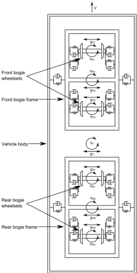
The current study considers a vehicle model with a full length body no longer constrained in yaw, plus two bogies with the accompanying four wheelsets, Figure 1. As with previous studies this model only considers the lateral and yaw directions, as the longitudinal and vertical effects can be satisfactorily neglected, Wickens (2003).

Fig. 1. Vehicle system plan view model

A detailed description of the development of railway vehi-cle dynamics can be found in Garg and Dukkipati (1984), with the rigid body dynamics for the simulation model given below by equations 1 to 14. These equations encom-pass lateral and yaw dynamics for the four wheelsets, two bogies and the vehicle body.

mF Fy¨F F =FLyF F +FRyF F +FsyF F +FgF F (1)

IF Fψ¨F F =FLyF FRLxF F−FLxF FRLyF F

+FRyF FRRxF F −FRxF FRRyF F

+MsψF F +MgF F

(2) mF Ry¨F R=FLyF R+FRyF R+FsyF R+FgF R (3)

IF Rψ¨F R=FLyF RRLxF R−FLxF RRLyF R

+FRyF RRRxF R−FRxF RRRyF R

+MsψF R+MgF R

(4) mRFy¨RF =FLyRF +FRyRF +FsyRF +FgRF (5)

IRFψ¨RF =FLyRFRLxRF−FLxRFRLyRF

+FRyRFRRxRF −FRxRFRRyRF

+MsψRF+MgRF

(6) mRRy¨RR=FLyRR+FRyRR+FsyRR+FgRR (7)

IRRψ¨RR=FLyRRRLxRR−FLxRRRLyRR

+FRyRRRRxRR−FRxRRRRyRR

+MsψRR+MgRR

(8) mF By¨F B=−(FsyF F+FsyF R+FsyV F) (9)

IF Bψ¨F B =−(MsψF F+MsψF R+MsyV F

+L(FsyF F −FsyF R))

(10) mRBy¨RB=−(FsyRF+FsyRR+FsyV R) (11)

IRBψ¨RB=−(MsψRF+MsψRR+MsyV R

+L(FsyRF−FsyRR))

(12) mVy¨V =FsyV F +FsyV R (13)

IVψ¨V =MsψV F +MsψV R (14)

where Fijkl, Rijkl, Miψkl are the forces (creep,

gravita-tional and suspension), positions and moments, mkl is

the mass, Ikl is the moment of inertia, ykl is the lateral

position, ψkl is the yaw angle; where i =L(eft), R(ight),

s(uspension); j =x(longitudinal), y (lateral); k =F(ront

bogie), R(rear bogie), V(vehicle); l =F(ront wheelset),

R(rear wheelset), B(ogie)

The accompanying suspension forces and moments (for small angles) for the primary and secondary suspension are given by equations 15 to 26.

FsyF F =ky1y_BF +k_y1Lψ_BF−k_y1y_{F F} +fy1y˙BF +fy1Lψ˙BF −fy1y˙F F (15) MsψF F =kψ1(ψ_BF −ψ_{F F}) +f_ψ1( ˙ψ_BF−ψ˙_{F F}) (16) FsyF R=ky1y_BF −k_y1Lψ_BF−k_y1y_{F R} +fy1y˙BF −fy1Lψ˙BF −fy1y˙F R (17) MsψF R=kψ1(ψBF −ψF R) +fψ1( ˙ψBF−ψ˙F R) (18) FsyRF =ky1yBR+ky1LψBR−ky1yRF +fy1y˙_BR+f_y1Lψ˙_BR−f_y1y˙_RF (19) MsψRF =kψ1(ψ_BR−ψ_RF) +f_ψ1( ˙ψ_BR−ψ˙_RF) (20) FsyRR=ky1y_BR−k_y1Lψ_BR−k_y1y_RR +fy1y˙_BR−f_y1Lψ˙_BR−f_y1y˙_RR (21) MsψRR=kψ1(ψ_BR−ψ_RR) +f_ψ1( ˙ψ_BR−ψ˙_RR) (22) FsyV F =−ky2y_V −f_y2y˙_V +k_y2y_BF+f_y2y˙_BF −ky2cψ_V −f_y2cψ˙_V (23) MsψV F =−ky2c 2 ψV −fy2c 2_˙ ψV +ky2cy_V +f_y2cy˙_V −ky2cy_BF −f_y2cy˙_BF (24) FsyV R=−ky2y_V −f_y2y˙_V +k_y2y_BR+f_y2y˙_BR +ky2cψ_V +f_y2cψ˙_V (25) MsψV R=−ky2c 2 ψV −fy2c 2_˙ ψV −ky2cy_V −f_y2cy˙_V −ky2cy_BR−f_y2cy˙_BR (26)

where kmn and fmn are the suspension stiffness and

damper coefficients; with m= y(lateral) or ψ(yaw); n=

1(primary suspension), 2(secondary suspension).

Creep forces fundamentally provide the guidance mech-anism for the wheelsets. These forces are generated in reaction to the creeps (or slips) in the rolling contact of the wheel-rail interface in normal running, these are relative

velocities of the wheel and the rail in the contact area and are defined as

si=

wi

V , i=x, y (27)

where V is the forward velocity of the wheelset,wi is the

creep (slip) velocity in the relevant direction (where xis

longitudinal direction andyis lateral direction), where this

is defined as

wi =Vw−Vr, i=x, y (28)

whereVw is the velocity of the wheel through the contact

patch, andVris the velocity of the rail through the contact

patch. Creep generation is a highly nonlinear process, however effects of hysteresis can be ignored due to this being a single direction rolling contact.

Normal practice for wheel-rail contact modelling is to lin-earise the creep forces generated in the model based upon Kalker coefficients, Kalker (1967). Due to the importance here of modelling the non-linear adhesion characteristics up to and beyond the creep saturation, use is made of the contact force model developed in Polach (2005). This is essentially a practical curve fitting mechanism, where the creep force (excluding spin effects) are calculated as

F = 2Qµ π _ǫ 1 +ǫ2 +arctanǫ (29)

whereQis the wheel load, with

ǫ=2 3

Cπa2

b

Qµ s (30)

where C is the proportionality coefficient of the contact

sheer stiffness N/m3

. Kalker coefficients can be used for this purpose, where for the longitudinal direction

ǫx=

1 4

Gπabc11

Qµ sx (31)

where sxis the longitudinal component of the total creep

s

s=qs2

x+s2y (32)

The forcesFx,Fyin the longitudinal and lateral directions

are

Fi=F

si

s, i=x, y (33)

and the adhesion coefficients fi=

Fi

Q, i=x, y (34)

The friction coefficients rely upon the slip velocity, where µ=µ0

(1−A)e−Bw

+A

(35)

A is the ratio of limit friction coefficient at infinity slip

velocityµ∞ to the maximum friction coefficientµ0

A=µ∞ µ0

(36) For large creep applications the force is worked out using

reduction factors,kAin the area of adhesion andkS in the

area of slip, as F =2Qµ π _k Aǫ 1 + (kAǫ)2 +arctan(kSǫ) , kS ≤kA≤1 (37) where k=kA+kS 2 (38)

Experimentation has shown that, contrary to expectation from theoretical models such as that of Kalker, Kalker

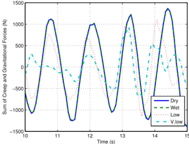
(1967), the initial slope of the creep curve varies with different adhesion levels, Pearce and Rose (1985), Harrison and McCanney (2002). Four levels of adhesion are defined in this study as dry, wet, low and very low conditions. The accompanying constants are given in Table 1 and the creep curves are given in Figure 2. This varying slope means that different adhesion levels should be feasibly detected without the system becoming saturated. The effect of varying the adhesion levels on the running system is shown in Figure 3. This shows the sum of the lateral creep forces and gravitational stiffnesses for the rear bogies front wheelset and demonstrates that for the same system disturbance (i.e. the lateral position of the track), the creep forces generated reduces as the friction levels reduce, meaning that detection of changes of adhesion level is feasible in practice.

Model parameter Dry Wet Low Very Low

kA 1.00 1.00 1.00 1.00

ks 0.40 0.40 0.40 0.40

µ0 0.55 0.30 0.06 0.03

A 0.40 0.40 0.40 0.40

B 0.60 0.20 0.20 0.10

Table 1. Polach contact model parameters

0 0.002 0.004 0.006 0.008 0.01 0 0.05 0.1 0.15 0.2 0.25 0.3 0.35 0.4 0.45 0.5 CREEPAGE COEFF. OF FRICTION DRY WET LOW VERY LOW

Fig. 2. Creep curves for varying adhesion conditions

10 11 12 13 14 15 −1500 −1000 −500 0 500 1000 1500

Sum of Creep and Gravitational Forces (N)

Time (s)

Dry Wet Low V.low

3. CREEP FORCE ESTIMATION TECHNIQUE This study applies a Kalman-Bucy filter technique (Kalman (1960)) as developed for the half vehicle model in Charles et al. (2008), to the full vehicle model of the previous section. As mentioned earlier this method attempts to estimate the total reactive creep and gravitational forces generated at the wheel rail interface. The size of these creep forces can then be analysed to determine the level of adhesion present, and the impact of the rail vehicle upon the track infrastructure.

The Kalman-Bucy filter model uses simplified versions of the system equations 1 to 8. As previous studies high-lighted, the detection technique used here can not dif-ferentiate between left and right creep forces, and the gravitational stiffness present. Therefore these are brought together as one state to be estimated, these are now

mF Fy¨F F =FF F +FsyF F (39) IF Fψ¨F F =MF F +MsψF F (40) mF Ry¨F R=FF R+FsyF R (41) IF Rψ¨F R=MF R+MsψF R (42) mRFy¨RF =FRF +FsyRF (43) IRFψ¨RF =MRF +MsψRF (44) mRRy¨RR=FRR+FsyRR (45) IRRψ¨RR=MRR+MsψRR (46)

where for the purposes of the filter, the following assump-tions are made

˙

FF F = ˙FF R= ˙FRF = ˙FRR= 0 (47)

˙

MF F = ˙MF R= ˙MRF = ˙MRR= 0 (48)

For this proof of concept work it is assumed that all of the states can be measured. Practically this will not be possible, so later stages of the work will look into reducing the number of states to be measured, and gauging how many can be estimated without detrimentally affecting the creep force estimation quality. The Kalman-Bucy filter, Grewal and Andrews (2001), is a very well known state space method, where the state equation is defined as

˙

x=Akx+Bku+z (49)

where xis the state vector, ˙xis the rate of change of the

state vector,z is the Gaussian noise source on each of the

state vectors, Ak is the state matrix andBk is the input

matrix. The output equation for the system is defined as

y=Ckx+Dku+v (50)

where y is the output vector, v is the Gaussian noise on

the output vector,Ck is the output matrix andDk is the

input matrix.

Design choices are made by selecting covariance matrices of the state and the input. These define how much noise is present in the system, therefore affecting the output of the system due to the model measurements not exactly matching the system.

The filter algorithm can be split into two sections. The first section calculates how much to adapt the filter to changes in the system. K=P CT KR −1 (51) ˙ P =AkP+P ATk −KRKT +Q (52)

where K is the ‘Kalman gain’, P is the error covariance

which in this continuous case the initial conditions of which require setting.

The second part is updating the estimates. The estimated state and output are then calculated simultaneously as

ˆ

y=Ckxˆ+Dku (53)

˙ˆ

x=Akxˆ+Bku+K(y−yˆ) (54)

where ˆy is the estimated output and ˆx is the estimated

state.

In this example, it is assumed that there is no system

input, and the filter becomes output only, thereforeCk=

Dk = 0. Where the state vector is defined as

x= [yF Fy˙F F ψF Fψ˙F FyF Ry˙F RψF Rψ˙F R · · · · · · yBF y˙BFψBF ψ˙BFyRFy˙RF · · · · · · ψRFψ˙RFyRRy˙RRψRRψ˙RR · · · · · · yBRy˙BRψBRψ˙BRyV y˙V · · · · · · ψV ψ˙V FF FFF RFRFFRR · · · · · · MF FMF RMRF MRR]T (55)

The primary tuning parameter here is the Q matrix,

defined as a diagonal matrix, where

Q=diag[1 1 1 1 1 1 1 1 1 1 1 1 1 1 · · · · · ·1 1 1 1 1 1 1 1 1 1 1 1 1 1 · · · · · ·1e9 1e9 1e9 1e9 1e9 1e9 1e9 1e9 ] (56) The high values associated with the last eight positions in the matrix assign uncertainty to the assumptions of equations 47 and 48, allowing the filter to adapt the state estimates to the creep force levels.

Figure 4 show results of the filter output compared to the modelled total lateral creep forces for the rear wheelset of the front bogie, by inspection this shows good correlation for the specific estimate. The simulation parameters are for dry friction and the model velocity is 20 m/s, with suspension parameters given in Table 2. The coefficient of

determination (R2

) values for the four lateral creep forces from the simulations with different levels of adhesion are shown in Table 3, where this is calculated as

R2 = 1− σ 2 (ǫ(t)) σ2_(y(t)) (57) whereσ2

(ǫ(t)) is the variance of the residuals andσ2

(y(t))

is the variance of the output, Ljung (1999). This shows that there is some reduction in the quality of the creep force estimation as the friction level reduces. This is due to the nonlinear effects of the creep force saturation becoming more prominent as the adhesion level reduces. The best estimates are achieved overall are for the front bogie rear wheelset creep forces. The estimator can also be shown to track adhesion changes in real time, Figure 5. This Figure demonstrates a simple interpolation scheme of the adhesion conditions in the simulation model, and how the estimator successfully track the changes to the creep force level. This is the early stages of this investigation and further work will look into how these estimates are affected by removing some of the measured signals.

Parameter Description Value Units

fy1 primary lateral damper

CoE

0 Ns/m

fψ1 primary yaw damper

CoE 0 Nms fy2 secondary lateral damper CoE 0.06e6 Ns/m

Ib bogie yaw inertia 3500 kgm2 Iv vehicle yaw inertia 30000 kgm2 Iw wheelset yaw inertia 700 kgm2 ky1 primary lateral

stiff-ness

40e6

N/m

ky2 secondary lateral

stiff-ness

0.1e6

N/m

kψ1 primary yaw stiffness 2.5e6 Nm

mb bogie mass 2500 kg

mv vehicle mass 1250 kg

mw wheelset mass 22000 kg yF F front bogie, front

wheelset displacement

- m

yF R front bogie, rear wheelset displacement

- m

yRF rear bogie, front wheelset displacement

- m

yRR rear bogie, rear wheelset displacement

- m

ψF F front bogie, front wheelset yaw angle

- rad

ψF R front bogie, rear wheelset yaw angle

- rad

ψRF rear bogie, front wheelset yaw angle

- rad

ψRR rear bogie, rear wheelset yaw angle

- rad

Table 2. Model parameters

0 5 10 15 20 25 30 −8000 −6000 −4000 −2000 0 2000 4000 6000 8000

Sum of Creep and Gravitational Forces (N)

Time (s)

Original Estimate

Fig. 4. Estimation of the lateral creep forces

Creep force/ moment Dry R2 (%) Wet R2 (%) Low R2 (%) V.Low R2 (%) FF F 83.64 82.95 69.94 65.10 FF R 85.12 84.90 79.26 73.44 FRF 85.03 84.28 73.64 71.88 FRR 85.13 85.14 72.76 65.35 Table 3. Lateral creep forces fit quality

0 5 10 15 20 25 30 vlow low wet dry Time (sec) Adhesion condition Adhesion level 0 5 10 15 20 25 30 −1 −0.5 0 0.5 1x 10 4 Time (sec) Creep force (N)

Creep force and gravitational stiffness

Actual Estimate

Fig. 5. Varying adhesion estimation 4. FUTURE WORK

This study provides a strong theoretical background for a project on on-board detection of low adhesion which started in 2010, administered by the Rail Safety and Strategy Board (RSSB) with funding from the UK’s Rail Industry Strategic Research Program. The project has several facets: further development of the data processing algorithms as shown here; how these estimates can be translated into a useful understanding of the adhesion condition; fundamental research into creep characteristics at low creep values using a scale roller rig; and validation of the techniques through data generated by a multi-bodied

dynamic simulation package (such as VAMPIRER) and

data gathered from a full scale instrumented vehicle. The intention is also to consider the force estimation technique for many other applications. This could be used for assessing the performance of railway vehicles in terms of the wheel and rail geometric and wear characteristics, perhaps as part of a homologation process. As mentioned earlier this is considered a simpler and cheaper alternative to the use of load measuring wheels which is the current practice. Beyond a homologation process, the technique if applied to a large number, or the majority of the vehicles on the network could be used to help in the prediction wear of the wheel tread, wear of the rail head and it could also be used predict the occurrence of rolling contact fatigue. These latter two points which consider the condition of the infrastructure would require extremely accurate coordination of the position of the vehicle on the network to the forces being estimated, and a study would also have to be generated as to how these forces relate the presence of patterns of wear and fatigue phenomena.

5. CONCLUSIONS

This paper discussed development work of the creep force estimation technique around the wheel-rail interface. The primary aim of this research is to develop a real-time system for the estimation of creep forces that could be used to detect local adhesion conditions, and predict the wear generated on the vehicle and the rail infrastructure. Firstly this paper discussed the development of a full vehi-cle body non-linear contact mechanics model of the lateral

and yaw dynamics of the system. This was performed as previous studies highlighted that some of the lateral creep forces and creep moments gave a better estimation than others, and this needed to be investigated in a more representative model of a rail vehicle system.

It then discussed the Kalman-Bucy filter method used to estimate the lateral creep forces and the yaw creep moments of the four wheelset in the model, and how these have given successful estimations in simulations.

Finally the future direction of the project was highlighted with further development potential of the algorithm given, and an explanation of the methods of validation that will be used, by data generated in multi-bodied dynamics simulation software and through track testing. Suggestions were also given for other applications of the creep force estimations.

ACKNOWLEDGEMENTS

The authors would like to thank Rail Research United Kingdom (RRUK) and the Engineering and Physical Sci-ence Research Council (EPSRC) who funded this research.

REFERENCES

Bombardier (2010). Orbita - predictive asset

management, the future of fleet maintenance.

http://www.bombardier.com/en/transportation/ accessed 7th April 2010.

Charles, G., Goodall, R., and Dixon, R. (2008). Model-based condition monitoring at the wheel-rail interface.

Vehicle System Dynamics, 46(1), 415–430.

Garg, V. and Dukkipati, R. (1984). Dynamics of Railway

Vehicle Systems. Academic Press, first edition.

Grewal, M. and Andrews, A. (2001). Kalman

Filter-ing: Theory and Practice Using MATLAB. Wiley-Interscience Publications, second edition.

Harrison, H. and McCanney, T. (2002). Recent devel-opments in coefficient of friction measurements at the

rail/wheel interface. Wear, 253(1), 114–123.

Hussain, I. and Mei, T. (2010). Multi kalman filtering approach for estimation of wheel-rail contact

condi-tions. InProceedings of the UKACC control conference,

Coventry.

Kalker, J. (1967). On the Rolling Contact of Two Elastic

Bodies in the Presence of Dry Friction. Ph.D. thesis, Delft University of Technology, Delft, Netherlands. Kalman, R. (1960). A new approach to linear filtering and

prediction. Transactions of ASME - Journal of Basic

Engineering, 35–45.

Li, P., Goodall, R., Weston, P., Ling, C., Goodman,

C., and Roberts, C. (2006). Estimation of railway

vehicle suspension parameters for condition monitoring.

Control Engineering Practice, 15:43-55.

Ljung, A. (1999). System Identification, Theory for the

User. Prentice Hall, second edition.

Mei, T. and Li, H. (2008). Measurement of vehicle ground

speed using bogie based inertial sensors. IMECHE

proceedings, Part F - Rail and Rapid Transit, 222(2), 107–116.

Pearce, T. and Rose, K. (1985). Measured force-creep rela-tionships and their use in vehicle response calculations. InProceedings of the IAVSD 9th Symposium, Linkoping.

Polach, O. (2005). Creep forces in simulations of traction

vehicles running on adhesion limit. Wear, 258(1), 992–

1000.

Vasic, G., Franklin, F., and Kapoor, A. (2003). New

rail materials and coatings. Technical Report

RRUK/A2/1, University of Sheffield, prepared for RSSB. http://portal.railresearch.org.uk/RRUK/Shared %20Documents/rssba2a.pdf.

Ward, C., Goodall, R., and Dixon, R. (2010a).

Wheel-rail profile condition monitoring. InProceedings of the

UKACC control conference, Coventry.

Ward, C., Weston, P., Stewart, E., Li, H., Goodall, R., Roberts, C., Mei, T., Charles, G., and Dixon, R. (2010b). Condition monitoring opportunities using

ve-hicle based sensors. In press: IMechE proceedings, Part

F: Rail and Rapid Transit.

Wickens, A. (2003).Fundamentals of Rail Vehicle

Dynam-ics: Guidance and Stability. Swets and Zeitlinger, first edition.

Xia, F., Cole, C., and Wolfs, P. (2008). Grey box-based inverse wagon model to predict wheel-rail contact forces

from measured wagon body responses. Vehicle System

Dynamics, 46(Supplement), 469–479.