Identifying the range of distance over which open space affects housing values
Seong-Hoon Cho Corresponding author
Assistant Professor
Department of Agricultural Economics University of Tennessee
314-A Morgan Hall Knoxville, TN 37996-4518 Tel: +1 865 974 7408 Fax: +1 865 974 9492 e-mail: [email protected] Dayton M. Lambert Assistant Professor
Department of Agricultural Economics University of Tennessee
Seung Gyu Kim Graduate Research Assistant Department of Agricultural Economics
University of Tennessee William M. Park
Professor
Department of Agricultural Economics University of Tennessee
Roland K. Roberts Professor
Department of Agricultural Economics University of Tennessee
Selected Paper prepared for presentation at the Southern Agricultural Economics Association Annual Meeting, Orlando, FL, February 6-9, 2010
Copyright 2010 by Cho, Lambert, Kim, Park, and Roberts. All rights reserved. Readers may make verbatim copies of this document for non-commercial purposes by any means, provided
Identifying the range of distance over which open space affects housing values Abstract
This research uses a sequence of hedonic housing price regressions to estimate open space amenity values. The iterative approach empirically identifies the range of distance over which open space affects housing values. After controlling for numerous other factors in the spatial hedonic model, simple functional relationships were established between the implicit prices of developed open space, forest-land open space, and agriculture-wetland open space and the buffer radius of the area surrounding a given location. In the case of Nashville-Davidson County, Tennessee, households place a positive value on additional developed open space and forest-land open space up to distances of 2.2 miles and 1.5 miles, respectively, and a negative value for additional agriculture-wetland open space up to 0.8-miles from their location.
Implicit-price-buffer-size functional relationships found in this study may be useful to local planners or policymakers. For example, local policymakers can identify the set of homeowners who would receive positive amenity values from developed open space or from preservation of forest-land open space, given the distance thresholds determined. Estimates of amenity and disamenity values of homeowners would allow the aggregate value generated by a particular open-space site to be estimated. The aggregate value consumers receive reflects the value residents place on neighborhood open space and is an estimate of the value of open-space as a public good. Thus, decision makers can prioritize specific open-space establishment or preservation decisions by not only accounting for the costs of establishing or preserving open space, but also estimating the public value of open space.
Keywords agriculture-wetland open space, amenity value, developed open space, forest-land open space, hedonic spatial model
1 Introduction
Hedonic housing price studies usually define the size of open-space buffers using ad hoc
methods. For example, Geoghegan et al. (2003) used 100 and 1,600 meter radius buffers around properties to estimate open-space amenity values. The authors assumed these radii captured the amenity value of the view from a property afforded by open space, including the value of open-space amenities within walking distance. Acharya and Bennett (2001) defined a variable measuring open space as the percentage of land circumscribed by a 1,600-meter buffer, with no apparent justification. Similarly, Nelson et al. (2004) used three open-space buffer radii: 0.1, 0.25, and 1.0 miles. They assumed the 0.1-mile radius buffer captured the amenities of visible open space, the 0.25-mile radius the amenities associated with neighborhood blocks, and the 1.0-mile radius buffer captured the amenities enjoyable on an “easy walk” around the neighborhood. Following their assumption, Cho et al. (2009) used 1.0 mile radius buffer to capture demand for public open space within easy walking distance. Irwin (2002) defined an open-space variable as the percentage of land in a 400-meter buffer. Lichtenburg et al. (2007) defined open-space area using rings with radii of 0.5, 1, and 2 miles, without explanation. Irwin et al. (2003) used different sized donut-shaped buffers in a model of suburban land use change. The ad hoc ranges for these buffers were 0 to 200 meters, 200 to 400 meters, 400 to 800 meters, and 800 to 1,600 meters.
To the best of our knowledge, there are no objective methods in the open-space valuation literature that represent an adequate procedure for determining open-space buffer size.
over distance could provide policy makers with a metric that avoids a priori judgments on this relationship.
A data–driven approach is used to estimate the relationship between the amenity values attributed to three types of open space in the Nashville-Davidson County, Tennessee
metropolitan area, i.e., developed open space, forest land open space, and agriculture-wetland open space, over a range of buffer sizes. A sequence of 50 hedonic spatial regressions using single family housing sales transactions generates implicit price estimates for the three open-space types by increasing the radius of the buffer by 0.1 mile up to 5 miles. The resulting coefficients for the open-space variables were used to determine a threshold beyond which the marginal value of additional open space was zero.
The next section details the empirical methods and procedures. A procedure for determining the range of open-space valuation is introduced, followed by the spatial hedonic model used to estimate the relationship between housing price and open space. The data are then described, highlighting the geographical information system (GIS) data sets used in the analysis. The empirical results are discussed next, and the last section concludes.
2 Methods and Empirical Model
Previous research has sequentially measured open space using land cover data (e.g., Acharya and Bennett 2001; Nelson et al. 2004; Poudyal et al. 2009). Land cover data, including the national land cover database (NLCD), has some distinct advantages. The NLCD data base is standardized with respect to definitions used to classify satellite images into specific land use categories. The information is also publicly available to researchers. There may be drawbacks, however, to using
NLCD data (Kline et al. 2009). Concern has been expressed that the NLCD does not accurately reflect low density residential development patterns, particularly in rural areas, when land use change is the subject of inquiry (Irwin and Bockstael 2007). Parcel level data may also provide a more accurate measure of site-specific open space (Geoghegan et al. 2003; Irwin et al. 2003). However, the focus of this research is not on changes in land use per se, but on the valuation of open space in an established urban/suburban housing market. In this case, because aerial remote images of urban areas are generally accurately interpreted, a static picture of the urban physical characteristics is likely sufficient (Irwin and Bockstael 2007).
Land cover information was acquired from 2001 Landsat 7 imagery (NLCD 2001) for 21 mutually exclusive land use categories at a resolution of 30 m by 30 m. Individual parcel data were for 2006 (MPD 2009). Given the time difference between the parcel data and the 2001 Landsat 7 imagery, some sales transactions occurring after 2001 likely affected the amounts of developed open space, forest land, and agriculture-wetland observed in 2001.
To minimize the time difference, the 2001 NLCD images were updated using individual parcel data. This entailed two steps. First, ‘open space’ was defined by placing each 30 m × 30 m NLCD pixel into one of the three open-space categories. The NLCD classification that included large-lot single-family housing units, parks, golf courses, and vegetation planted in developed settings for recreation, erosion control, or aesthetic purposes was categorized as “developed open space”. The pixels in the three NLCD classifications of deciduous forest, evergreen forest, and mixed forest were categorized as “forest-land open space”. The category of “agriculture-wetland open space” included the six NLCD classifications of shrub/scrub, grassland/herbaceous,
pasture/hay, cultivated crops, woody wetlands, and emergent herbaceous wetlands. A sequence of 50 buffers was constructed around each sales transaction. Areas were aggregated for each
open-space type within each buffer. Second, parcels developed during the 2002-2005 period were removed from the aggregated areas of open space. Parcels developed for single family housing greater than 10 acres were not excluded from the open-space areas because the significant lot size of these parcels may provide amenity values to neighbors similar to other developed open space.
2.1 Iterative Procedure for Determining the Range of Open-space Impact
A four-step procedure was employed to estimate the marginal change in the implicit price of open space as a function of distance from a sales transaction location. The first step entailed construction a sequence of open-space buffers for buffer radii of increasing distance around the location of each sales transaction as follows: We constructed 50 buffers at i = 1,…, 2,813 sales transactions, where r = 0.1, 0.2, …, 5.0 was the radius originating from location i (in miles). Areas of developed open space AD, forest-land open space AF, and agriculture-wetland open space AA within buffer r were estimated as the cumulative area of the pixels defined as
‘developed open space’, ‘forest-land open space’, and ‘agriculture-wetland open space’ within a radius of r from the sales transaction, given the land use definitions above. For example, the areas within the first buffer surrounding a sales transaction location included the aggregate areas for each of the three open-space types within an r = 0.1-mile radius and the 50th buffer included the areas of these open-space types within an r = 5.0-mile radius of the transaction. The process is visualized in Fig. 1.
In the second step, the hedonic price model was estimated 50 times, each time replacing the three open-space variables with those for the next larger buffer. Consider a hedonic model of housing sale prices at location i (yi):
ln Dln D Fln F Aln A
i i i t i i i
y xβ A A A (1)
where lnyi is the natural log of the sale price of house i, xiis a vector of structural, census block-group, high school district and other spatial market information, βis a vector of parameter, and θs are the scalar parameters for the open-space types, and εi is a disturbance term. Because open space is largely determined by forces in the housing market and the housing price is a function of open space, a system of simultaneous equations is typically used to represent the relationship between open space and housing price (Irwin and Bockstael 2001; Geoghegan et al. 2003; Walsh 2007). The Durbin-Wu-Hausman test was conducted for each open-space type for each regression to test the simultaneity hypothesis (Davidson and MacKinnon 1993). Failure to reject the null hypothesis suggested that the open-space measures are statistically exogenous.
In the third step, the marginal implicit prices for the three types of open space (pD,p pF, A) were estimated from each of the 50 regressions. For example, the marginal implicit price of developed open space is the partial derivative of the hedonic price function with respect to developed-open-space area when price and area are logged:
ˆ ˆ ln ˆ ln ˆ ln ˆ e ˆ ˆ ˆ , D D F F A A i t Ai t Ai t Ai D i D i D D D i i i y y p A A A xβ (2)
where “^” denotes a consistent estimate of (β,). The estimated parameter ˆDis developed open-space elasticity of housing price because they were estimated in a log-log relation. For example, using the mean of the predicted sale price of a house ($201,136) and the mean of
Davidson County, and the coefficient for developed open space estimated from equation 2 (0.125), the average marginal implicit price within a 2-mile buffer is $12.52 per acre of
developed open space (=0.125 $201,136) / 2,008 acres). This marginal implicit price suggests that increasing developed open space by 1 acre within a 2-mile radius buffer increases the average value of a house by $12.52, ceteris paribus.
Because of the construction of how the marginal implicit price for developed open space (pD) was calculated each iteration, the implicit price of an acre of developed open space is expected to decrease as the size of the buffer increases as long as ˆDremains equal or lower than one (which was the case in our estimates). A fairly constant mean of the predicted sale price of a house (the numerator) and increasing developed open-space area (the denominator) in the equation 2,
ˆ ˆD i D i y A
, causes a decrease the implicit price of developed open space with increasing buffer
sizes. Despite the expectation due to the calculation of the implicit price of developed open space, the relationship between the price of developed open space and the open-space buffer size is also predicated on the significance of the open-space parameters.
In the fourth step, an exponential curve was fitted by regression for each open-space type with the 50 estimated marginal implicit prices as the dependent variable and the 50 radii as the independent variable. The fitted curve for each open-space type was used to calculate percentage changes in predicted marginal implicit prices for each 0.1-mile increase in the buffer radius from r = 0.1 to 5.0 miles. A 5% change in the marginal implicit price was the tolerance criterion chosen for identifying the buffer radius beyond which open-space contributes little additional value to a house.
2.2 Estimation of the Spatial Hedonic Model
Spatial hedonic models are commonplace in empirical studies of housing and real estate markets (Bockstael 1996; Anselin 1998; Basu and Thibodeau 1998; Pace et al. 1998; Dubin et al. 1999; Fleming 1999; Gillen et al. 2001; Plantinga and Miller 2001; Geoghegan at al. 2003; Pace and LeSage 2004; Irwin and Bockstael 2007; Tian et al 2007). Some hedonic price studies assume that housing price at a given location is simultaneously determined by neighboring housing prices (Kim et al. 2003; Cohen and Coughlin 2007; Anselin and Lozano-Gracia 2008). These studies typically use a spatial process model (Whittle 1954), which includes an endogenous variable that accounts for spatial interactions between prices observed at transaction points, exogenous variables relating house attributes as well as geographic and demographic data to sale prices, and a disturbance term. The interactions are modeled as a weighted average of nearby sales transactions, and the endogenous variable accounting for the interactions is usually referred to as a spatially lagged variable. A relational matrix identifies connectivity between transactions, which differentiates spatial process models from other spatial regression methods. Anselin and Florax (1995) call this model a spatial autoregressive lag model of the first order (SAR[1]). Whittle’s spatial autoregressive lag model was popularized and extended by Cliff and Ord (1973, 1981), who distinguished models in which the disturbances follow a spatial autoregressive process. The general model contains a spatially lagged endogenous variable as well as spatially autoregressive disturbances in addition to exogenous variables, and is called a spatial
autoregressive model with autoregressive (AR) disturbance of order (1,1) (SARAR) (Anselin and Florax 1995); y = ρW1y + Xβ + ε, ε = λW2ε + u, u ~ iid(0, Ω), where W1 and W2 are (possibly identical) matrices defining interrelationships between spatial units, and E[uu′] = Ω. The reduced
form of the system makes clear how observations are globally correlated: y = (I - ρW1)-1Xβ + (I - ρW1)-1(I - λW2)-1u, with (I - ρW1)and (I - λW2) of the lag and error filters. Even when W is a sparse matrix with most off-diagonal elements zero, the “Leontief” inverses of the filters are full matrices. In effect, the lag process amplifies shocks transmitted through the errors between cross sectional units. When the W matrix is asymmetric, the model is heteroscedastic (Anselin 2003).
Full information maximum likelihood (FIML) (Anselin 1988) or general moment (GM) procedures (Kelejian and Prucha 2007; Anselin and Lozano-Gracia 2008) are typically used to estimate spatial process models as applied in hedonic price studies. The GM procedure has several advantages over FIML. First, the distributional assumption of normality is relaxed. Second, the GM procedure bypasses calculation of an n by n matrix determinant, which may be cumbersome with larger data sets. However, despite these desirable attributes, when error terms are heteroskedastic, estimation of the spatial error AR term (λ) using the GM approach under the assumption of homoskedasticity may produce biased and inconsistent estimates of the
autoregressive coefficient (Kelejian and Prucha 2007).
We use the GM procedure recently suggested by Kelejian and Prucha (2007) to estimate the (AR) parameter. The procedure is robust to nonspherical disturbances. The basic steps are
similar to the feasible generalized least squares approach outlined by Kelejian and Prucha (1999), which was first applied to actual household-level data by Bell and Bockstael (2000).
2.3 Neighborhood Spatial Weight Matrix
A spatial weight matrix identifying neighborhoods of observations was constructed by combining an inverse distance matrix with a first-order queen contiguity weight matrix
(Brasington and Hite 2005; Lipscomb 2007). First, point data were converted to Thiessen polygon data to build the queen continuity matrix. Thiessen polygons translate the spatial representation of the sales transactions from points to polygons, and are related to notions of spatial market areas (Anselin 1988). Second, an n by n matrix of inverse distances between each transaction was calculated. Finally, the element-wise matrix product of the Thiessen polygon and distance matrix defined neighborhood contiguity. Thus, interaction between transactions was hypothesized to occur within a given neighborhood of adjacent transactions, discounted by the distance between the sales locations. The same matrix was used to model the error and lag processes.
2.4 Control Variables in the Hedonic Model
To control for effects on housing price other than the effects of open space, the hedonic model included structural attributes of the house (i.e., lot size, age, brick siding, garage, number of stories, condition of structure, and finished area), census-block group variables (i.e., vacancy rate, unemployment rate, travel time to work, income, housing density, and rural-urban interface), distance measures to amenities (i.e., central business district, golf course, sidewalk, park, water body) or disamenities (i.e., railroads), and school districts (i.e., average composite score of American College Test (ACT) score by school district) (See Table 1 for the complete list of the variables and their definitions).
Because a premium for proximity to a water body is expected to be significantly different with and without a water view (Darling 1973; Plattner and Campbell 1978; Gillard 1981; Benson et al. 1997; Brown and Pollackowski 1997; Morton 1977; Muller 2009), a dummy variable
intended as a proxy for water view was constructed based on the assumption that this would be the case for houses located less than 100 meters from a water body. A dummy variable was also constructed to differentiate houses located on the rural-urban interface. This was done by identifying census block groups with mixed urban-and-rural houses.
3 Data
Five GIS data sets were used in the analysis: individual parcel data, satellite imagery data, census-block group data, high school district boundary data, and environmental feature data. The individual parcel data (sales price, lot size, and structural information) were obtained from the Metro Planning Department of Davidson County (MPD 2009) and the Davidson County Tax Assessor's Office. Data were for single-family house sales during the second quarter of 2006 in Nashville-Davidson County, Tennessee. County officials suggested that sales prices below $40,000 were likely gifts, donations or inheritances, and would therefore not reflect true market value. Officials also suggested that parcel records indicating a lot size of less than 1,000 square feet were likely in error. Consequently, transactions with either of these characteristics were eliminated from the sample data. These reductions left 2,813 observations to be used in the statistical analysis.
The NLCD from the multi resolution land characteristics consortium included the GIS map used to identify open space in the first step of the two step process (NLCD 2001). The boundary data for high school districts were obtained from MPD. Data on environmental features, such as water bodies and golf courses, were drawn from the ESRI (Environmental Systems Research Institute) Data and Maps 2006 (ESRI 2006). Other data on environmental features, such as shape
files for railroads and parks, were from MPD. The study area included 467 census block groups. Information from the census block groups was assigned to houses located within the boundaries of the block groups. The distance variables were created using the spatial join tool to measure the closest distance in ArcGIS 9.2. These variables represent the distance between parcel centroids and either the centroids of the nearest park, golf course, central business district (CBD) or water body, or the nearest point to the polylines representing railroads and sidewalks.
4 Empirical Results
4.1 Model Specification
The Durbin-Wu-Hausman test indicated failure to reject the null hypothesis that the open-space variables were statistically exogenous (5% level) for any buffer size or open-space type. Thus, the open-space variables were not considered to be statistically endogenous in the 50 hedonic regressions. Variance inflation factors (VIFs) were used to test for multicollinearity among the explanatory variables (Maddala 1992). A general rule of thumb is that multicollinearity may be a problem if the VIF is greater than 10 (Gujarati 1995). The highest VIF of 8.05 was for developed open space using the 5-mile radius buffer, and mean VIFs across the 50 regressions were
consistently lower than 2.5, suggesting that the standard errors of the parameter estimates were not seriously affected by multicollinearity.
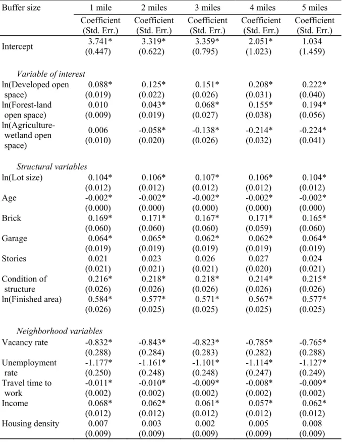
The results from five of the 50 SARAR (1,1) regressions are reported in Table 2 (1 to 5-miles radii in 1-mile increments). The R2s ranged between 0.70 and 0.71 for the heteroskedastic
regressions, as evidenced by the significant lag autoregressive (ρ) and error autocorrelation (λ) coefficients. Hereafter coefficients of variables are considered statistically significant if their p-values ≤ 0.05. With a few exceptions, only statistically significant variables are discussed in the remainder of this section.
4.2 Control Variables
The signs of all statistically significant coefficients associated with structural and neighborhood variables are consistent with expectations (Table 2). Newer houses and houses with bigger lots and finished areas, brick siding, garages, and better structural conditions are positively correlated with sales price. Houses located at the rural-urban interface and in neighborhoods with lower vacancy rates, lower unemployment rates, lower travel times to work, greater household incomes, and better high school districts are also valued more highly.
Significant coefficients for the distance variables show that being closer to a golf course, being further from a railroad, and having a water view are valued positively. The variable measuring the distance to the CBD was the only variable for which significance changed substantially with increased buffer sizes. The CBD variable was significant in the regressions with buffer radii of 0.1 to 2.1 miles, but not significant beyond 2.1 miles.
4.3 Range of Implicit Open-Space Price Decay
Developed open space is valued positively within buffers with radii of 0.5-miles or greater while forest-land open space is valued on and off between 0.1 and 1.5-mile radii and continuously
0.3, 0.4, and 0.5-mile radius buffers and continuously beyond the 1.5-mile radius buffer. The lack of significance for developed open space within buffers with radii less than 0.5 mile and intermittent significance for forest-land open space and agriculture-wetland open space within buffers with radii less than 1.5 miles was not totally unexpected based on previous literature. Geoghegan at al. (2003) found that open space measured inside a 1-mile radius either had no relationship with housing price or had a negative influence on property values.
In Nashville-Davidson County, most houses are clustered in subdivisions with little or no forest-land or agriculture-wetland open spaces. Alternatively, these subdivisions may include substantial numbers of large private lots that are defined in the data as developed open space. The likelihood of defining very much forest-land open space or agriculture-wetland open space within a 0.5-mile radius is relatively small and the value placed on someone else’s private lot as open space within 0.5-mile radius buffer may not be significant. Expanding the buffer increases the likelihood of including more open space and increases the likelihood of significance in the regression model. Another factor may be that amenities provided by developed open space in the form of parks or other outdoor venues in the immediate neighborhood (within a 0.5-mile radius) are offset by traffic, noise, and safety disamenities. While individuals may not enjoy being too close to developed open space, being able to access these areas easily, perhaps by walking, biking, or a short drive (outside a 0.5-mile radius) appears to have a premium attached to it (Fig. 2).
The finding that agriculture-wetland open space is apparently a disamenity was something of a surprise, but the particular characteristics of Nashville-Davidson County may explain this result. Less than 10% of Nashville-Davison County is classified as agriculture-wetland, and much of the agricultural land may be idle rather than actively farmed. This land category would
also include developed land that, as a result of urban decay, has reverted to grassland or scrub. Doss and Taff (1996) and Reynolds and Regalado (1998) also found a negative impact on property values of woody wetlands and emergent palustrine wetlands, which are included in the agriculture-wetland category. The higher disamenity values of agriculture-wetland open space closer to a house may emanate from livestock noise and/or odor associated with agricultural land or insect pests emerging from wetland.
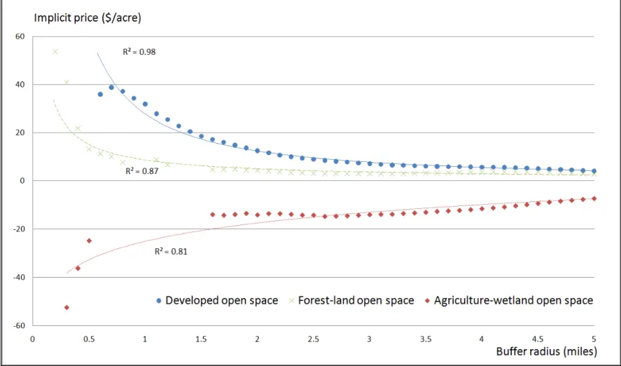
The estimated marginal implicit prices across different buffer sizes are presented in Fig. 2. Holding other factors constant, the marginal implicit price for developed open space decreases at a decreasing rate as the buffer size increases. The same pattern is observed with forest-land open space, but the implicit values of forest-land open space are positive for the 0.2, 0.3, 0.4, and 0.5-mile radius buffers and the implicit values of developed open space are larger than the implicit values of forest-land open space beyond the 0.5-mile radius buffer. The gap between the implicit value of developed open space and forest-land open space is at its highest at $30 per acre with the 0.8-mile radius buffer and decreases as the buffer increases beyond that size.
The marginal implicit price of an additional acre of developed open space is at its highest at $39 with a 0.7-mile radius buffer and decreases gradually as the buffer radius increases beyond that size (Fig. 2). In all, 45 of the 50 coefficients associated with the marginal implicit price of developed open space were significant. The relationship between the implicit price of open space and open-space buffer size is estimated as: Implicit price of developed open space/acre = 27.842
[radius of buffer] -1.17. The exponent is an elasticity, i.e., a 1% increase in radius of open-space buffer size corresponds with a 1.17% decrease in the value attributed to an additional developed open space associated with the increased buffer size.
The implicit price of an acre of forest-land open space is at its highest at $54 with a 0.2-mile buffer and decreases gradually as the buffer radius increases (Fig. 2). The relationship between the price of forest-land open space and the quantity of forest-land open space is summarized as follows: Implicit price of forest-land open space/acre = 8.657 [radius of buffer] -0.8. Therefore, a 1% increase in the radius of the open-space buffer corresponds with a 0.8% decrease in the value attributed to the additional forest-land open space associated with the increased buffer size.
Table 2 shows that both elasticities increase gradually with developed open-space area and forest-land open space as the buffer size was increased. The larger developed open-space elasticity of housing price and forest-land open-space elasticity of housing price in the larger buffer are expected because percent changes of developed open space and forest-land open space in a larger buffer correspond with larger quantities of developed open space and forest-land open space, respectively, while percent changes of developed open space and forest-land open space in smaller buffers correspond with smaller quantities of developed open space and forest-land open space, respectively.
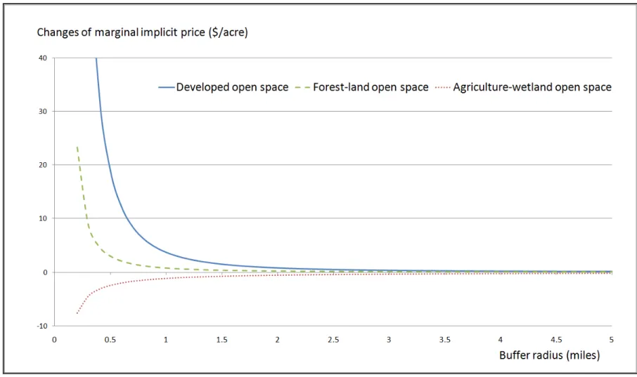
Fig. 3 shows the changes of marginal implicit prices (ΔMIP) of developed open space, forest-land open space, and agriculture-wetforest-land open space with respect to changes in successively larger radii denoted by ΔMIPD, ΔMIPF, and ΔMIPA, respectively. The ΔMIP is the slope of the relationship between the marginal implicit price of open space and open-space buffer size. The price-buffer size relationships decrease as the buffer size increases for developed open space and forest-land open space. For example, the ΔMIPD decreases by $2.94 as the buffer radius
increases from 1.0 to 1.1 mile and the MIPF decreases by $0.64 as the buffer radius increases from 1.0 to 1.1 mile.
The ΔMIPD and ΔMIPF reach the 5% tolerance criterion at buffer radii of 2.2-miles and 1.5-miles, respectively. These results suggest that, on average, little amenity value is derived from additional open space beyond that contained within 2.2 and 1.5-mile buffer radii for developed open space and forest-land open space, respectively. Beyond these distances, the ΔMIPD and
ΔMIPF essentially represents noise. This finding suggests the cutoff threshold for the range of distance over which households value developed open space is larger than the range of distance over which they value forest-land open space.
The ΔMIPA reaches the 5% tolerance criterion at a buffer radius of 0.8 mile. This result suggest that, on average, additional agriculture-wetland open space beyond that contained within a 0.8-mile buffer radius contributes little to reducing the disamenity value derived from
agriculture-wetland open space. Beyond this distance ΔMIPA essentially represents noise.
5 Conclusions
This research used a sequence of hedonic spatial regressions for a metropolitan housing market in the Southeastern United States to estimate the amenity values attributed to three types of open space. The regressions were estimated using a sequence of proxies for developed open space, forest-land open space, and agriculture-wetland open space. For each sales transaction, the areas of the three open–space types were calculated by summing their areas within a buffer of a given radius. The area of the buffer was sequentially increased by increasing the radius, thereby generating larger open-space areas surrounding each sales transaction. The hedonic model was estimated 50 times, replacing the open-space measures for buffers with successively larger radii. The implicit prices for each open-space type were calculated from the results of each regression.
Ex post analysis of the open-space coefficients suggest marginal implicit price functions for the three types of open space (with respect to house location) that decays as the area of open space increases. On average, after buffer radii of 2.2 miles and 1.5 miles, the positive marginal values attributed to additional developed open space and forest-land open space, respectively, approach zero and the negative marginal value of additional agriculture-wetland open space approaches zero at 0.8-mile from a house. After controlling for numerous other factors in the spatial hedonic model, simple functional relationships were established between the implicit prices of developed open space, forest-land open space, and agriculture-wetland open space and the buffer radius of the area surrounding a given location.
Implicit-price-buffer-size functional relationships may be useful to local planners or
policymakers. For example, local policymakers can identify the set of homeowners who would receive positive amenity values from developed open space or from preservation of forest-land open space, given the distance thresholds determined in this article. Estimates of amenity and disamenity values of homeowners would allow the aggregate value generated by a particular open-space site to be estimated. The aggregate value consumers receive reflects the value residents place on neighborhood open space and is an estimate of the value of open-space as a public good. Both public and private values should be considered when making decisions about establishing developed open space or preserving forest-land or agriculture-wetland open space. The market price of land is a private cost associated with open-space establishment or
preservation, while the public value of the open space is a benefit. Thus, decision makers can prioritize specific open-space establishment or preservation decisions by not only accounting for the costs of establishing or preserving open space, but also estimating the public value of open space using the methods contained in this article.
Three caveats associated with the methods used in this article should be mentioned. First, because the estimated amenity values are only a function of open-space area, ceteris paribus, variation in open-space quality is not addressed in the model, i.e., composition, shape, and historic value. Second, the amenity values of open space estimated in this study do not capture housing market dynamics, i.e., lags in the incorporation of amenity effects into prices, because the values from this hedonic model are estimated with one year’s sales data (Freeman 1993; Smith and Huang 1995). Third, in more congested areas, travel time may be a better measure of distance than the straight-line measure used in this study.
A clear need exist for further research into more detailed classification of open space to accommodate differences in quality. The aggregate developed open-space classification can be dissagregated into ballparks, which may generate disamenities tied to traffic, noise, and safety concerns, and other types of parks and golf courses, which may not produce those dissamenities. The agriculture-wetland open space may also be disaggregated into 1) large-scale animal
operations that may be associated with disamenities such as odor and noise, 2) agricultural cropland that may not have these dissamenities, and 3) wetlands that may generate insect pests such as mosquitoes. In addition, the spatial configuration of open space (e.g., patch density, which captures the degree of spatial heterogeneity) can be evaluated to determine how open-space quality affects the range of distance over which open open-space has value to homebuyers.
Reference
Acharya G, Bennett LL (2001) Valuing open space and land-use patterns in urban watersheds. J. Real Estate Finance Econ. 22 (2/3): 221-237.
Anselin L (1988) Spatial econometrics: methods and models. Kluwer Academic, Dordrecht. Anselin L (1998) GIS research infrastructure for spatial analysis of real estate markets. J. Hous.
Res. 9: 113-133.
Anselin L (2003) Spatial externalities, spatial multipliers and spatial econometrics. Int. Reg. Sci. Review 26, 153-166.
Anselin L, Florax R (1995) New direction in spatial econometrics. Springer, Berlin.
Anselin L, Lozano-Gracia N (2008) Errors in variables and spatial effects in hedonic house price models of ambient air quality. Empir. Econ. 34 (5): 5-34.
Basu S, Thibodeau, TG (1998) Analysis of spatial autocorrelation in house prices. J. Real Estate Finance Econ. 17: 61-85.
Bell KP, Bockstael NE (2000) Applying the generalized-moments estimation approach to spatial problems involving micro-level data. Review Econ. Stat. 82: 72-82.
Benson E, Hanson J, Schwartz A, Smersh G (1997) The influence of Canadian investment on U.S. residential property values. J. Real Estate Res. 13 (3): 231-249.
Bockstael NE (1996) Modeling economics and ecology: the importance of a spatial perspective. Am. J. Agric. Econ. 78: 1168-1180.
Brasington DM, Hite D (2005) Demand for environmental quality: a spatial hedonic analysis. Reg. Sci. Urban Econ. 35 (1): 57-82.
Brown G, Pollakowski H (1997) Economic value of shoreline. Review Econ. Stat. 59 (3): 272-278.
Cho S, Lambert DM, Roberts RK, Kim SG (2009) Demand for open space and urban sprawl: the case of Knox County, Tennessee. In: Paez A, Le Gallo J, Buliung R, Dall’Erba S (eds.) Progress in spatial analysis: theory and computation, and thematic applications. Springer, Berlin, In press.
Cliff AD, Ord JK (1973) Spatial autocorrelation. Pion, London.
Cliff AD, Ord JK (1981) Spatial processes - models and applications. Pion, London.
Cohen J P, Coughlin CC (2007) Spatial hedonic models of airport noise, proximity and housing prices. Federal reserve bank of St. Louis working paper no. 2006-026C.
Darling A (1973) Measuring benefits generated by urban water parks. Land Econ. 49: 22-34. Davidson R, MacKinnon JG (1993) Estimation and inference in econometrics. Oxford
University Press, New York.
Doss CR, Taff SJ (1996) The influence of wetland type and wetland proximity on residential property values. J. Agric. Res. Econ. 21: 120-129.
Dubin R, Pace RK, Thibodeau TG (1999) Spatial autoregression techniques for real estate data. J. Real Estate Lit. 7: 79-95.
ESRI, 2006. ESRI Data & Maps 2006.
http://webhelp.esri.com/arcgisdesktop/9.2/index.cfm?id=5637&pid=5635&topicname=A n_overview_of_ESRI_Data_and_Maps. Accessed 30 June 2009
Fleming MM (1999) Growth controls and fragmented suburban development: the effect on land values. Geogr. Inf. Sci. 15: 154-162.
Freeman AM (1993) Property Value Models, the measurement of environmental and resource values. Resources for the Future, Washington, DC.
Geoghegan J, Lynch L, Bucholtz S (2003) Capitalization of open space into housing values and the residential property tax revenue impacts of agricultural easement programs. Agric. Res. Econ. Review 32 (1): 33-45.
Gillard Q (1981) The effect of environmental amenities on house values: the example of a view lot. Prof. Geogr. 33 (2): 216-220.
Gillen K, Thibodeau TG, Wachter S (2001) Anisotrophic autocorrelation in house prices. J. Real Estate Finance Econ. 23: 5-30.
Gujarati D (1995) Basic econometrics, 3rd ed. McGraw-Hill, New York.
Irwin EG (2002) The effects of open space on residential property values. Land Econ. 78 (4): 465-480.
Irwin EG, Bell K, Geoghegan J (2003) Modeling and managing urban growth at the rural-urban fringe: a parcel-level model of residential land-use change. Agric. Res. Econ. Review 32 (1): 83-102.
Irwin EG, Bockstael NE (2001) The problem of identifying land use spillovers: measuring the effects of open space on residential property values. Am. J. Agric. Econ. 83 (3): 698-704. Irwin EG, Bockstael NE (2007) The evolution of urban sprawl: evidence of spatial heterogeneity and increasing land fragmentation. In Proceedings of the National Academy of Sciences 104: 20672-20677.
Kelejian HH, Prucha IR (1999) A generalized moments estimator for the autoregressive parameter in a spatial model. Int. Econ. Review 40: 509-533.
Kelejian HH, Prucha IR (2007) Specification and estimation of spatial autoregressive models with autoregressive and heteroskedastic disturbances. Working paper. Department of Economics, University of Maryland.
Kim CW, Phipps TT, Anselin L (2003) Measuring the benefits of air quality improvement: a spatial hedonic approach. J. Environ. Econ. Manag. 45 (1): 24-39.
Kline JD, Moses A, Azuma D, Gray A (2009) Evaluating satellite imagery-based land use data for describing forestland development in western Washington. Western J. Applied Forestry 24 (4): 214-222.
Lichtenburg E, Tra C, Hardie I (2007) Land use regulation and the provision of open space in suburban residential subdivisions. J. Environ. Econ. Manag. 54: 199-213.
Lipscomb CA (2007) An alternative spatial hedonic estimation approach. J. Hous. Res. 15 (2): 143-160.
MPD (2009) Metro Planning Department, Davidson County. http://www.nashville.gov/mpc. Accessed 30 June 2009
Maddala GS (1992) Introduction to econometrics. Prentice Hall, New Jersey.
Morton T (1977) Factor analysis, multicollinearity and regression appraisal models. The Apprais. J. October 578-588.
Muller NZ (2009) Using hedonic property models to value public water bodies: an analysis of specification issues. Water Resour. Res. 45.
Nelson N, Kramer E, Dorfman J, Bumback B (2004) Estimating the economic benefit of landscape pattern: a hedonic analysis of spatial landscape indices and a comparison of build-out scenarios for the protection of ecosystem functions. Working paper, Institute of Ecology, University of Georgia.
NLCD (2001) National Land Cover Database 2001.
Pace RK, Barry R, Clapp JM, Rodriguez M (1998) Spatial autocorrelation and neighborhood quality. J. Real Estate Finance Econ. 17(1): 15-33.
Pace RK, LeSage JP (2004) Spatial statistics and real estate. J. Real Estate Finance Econ. 29: 147-148.
Plantinga AJ, Miller DJ (2001) Agricultural land values and the value of rights to future land development. Land Econ. 77: 56-67.
Plattner R, Campbell T (1978) A study of the effect of water view on site value. Apprais. J. January 20-25.
Poudyal NC, Hodges DG, Cordell HK (2009) The role of natural resource amenities in attracting retirees: implications for economic growth policy. Ecol. Econ. 68 (1-2): 240-248.
Reynolds J, Regalado A (1998) Wetlands and their effects on rural land values. State Paper 98-2, University of Florida, Institute of Food and Agriculture Sciences, Gainesville, Florida. Smith VK, Huang JC (1995) Can markets value air quality? A meta-analysis of hedonic property
value models. J. Political Econ. 103 (1): 209-227.
Tian G, Yang Z, Zhang Y (2007) The spatio-temporal dynamic pattern of rural residential land in China in the 1990s using landsat TM images and GIS. Environ Manag. 40: 803-813. Walsh R (2007) Endogenous open space amenities in a locational equilibrium. J. Urban Econ. 6
(2): 319-344.
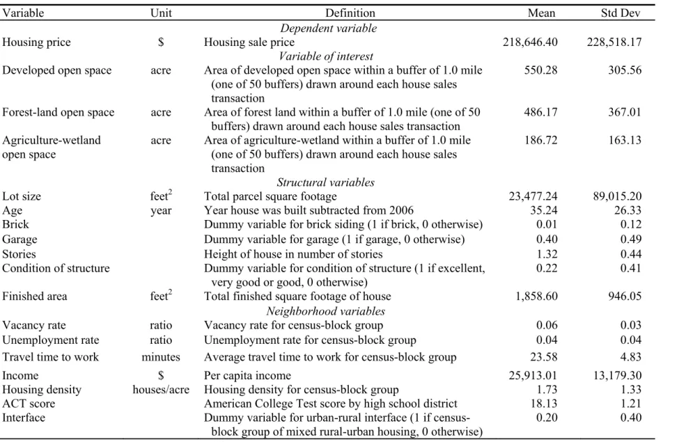
Table 1 Variable names, definitions, and descriptive statistics
Variable Unit Definition Mean Std Dev
Dependent variable
Housing price $ Housing sale price 218,646.40 228,518.17
Variable of interest
Developed open space acre Area of developed open space within a buffer of 1.0 mile (one of 50 buffers) drawn around each house sales transaction
550.28 305.56 Forest-land open space acre Area of forest land within a buffer of 1.0 mile (one of 50
buffers) drawn around each house sales transaction
486.17 367.01 Agriculture-wetland
open space
acre Area of agriculture-wetland within a buffer of 1.0 mile (one of 50 buffers) drawn around each house sales transaction
186.72 163.13
Structural variables
Lot size feet2 Total parcel square footage 23,477.24 89,015.20
Age year Year house was built subtracted from 2006 35.24 26.33
Brick Dummy variable for brick siding (1 if brick, 0 otherwise) 0.01 0.12
Garage Dummy variable for garage (1 if garage, 0 otherwise) 0.40 0.49
Stories Height of house in number of stories 1.32 0.44
Condition of structure Dummy variable for condition of structure (1 if excellent, very good or good, 0 otherwise)
0.22 0.41
Finished area feet2 Total finished square footage of house 1,858.60 946.05
Neighborhood variables
Vacancy rate ratio Vacancy rate for census-block group 0.06 0.03
Unemployment rate ratio Unemployment rate for census-block group 0.04 0.04
Travel time to work minutes Average travel time to work for census-block group 23.58 4.83
Income $ Per capita income 25,913.01 13,179.30
Housing density houses/acre Housing density for census-block group 1.73 1.33
ACT score American College Test score by high school district 18.13 1.21
Variable Unit Definition Mean Std Dev
Distance variables
Distance to CBD feet Distance to central business district 39,994.07 18,393.56
Distance to golf course feet Distance to nearest golf course 20,882.59 12,305.63
Distance to railroad feet Distance to nearest railroad 6,589.51 5,751.50
Distance to sidewalk feet Distance to nearest sidewalk 909.64 1,622.45
Distance to park feet Distance to nearest park 5,654.53 3,901.96
Water view Dummy variable indicating viewable water body (1 if
water body is within 100m, 0 otherwise)
Table 2 Results for the spatial hedonic models for buffers with radii of mile to 5-mile in 1-mile increments
Buffer size 1 mile 2 miles 3 miles 4 miles 5 miles
Coefficient (Std. Err.) Coefficient (Std. Err.) Coefficient (Std. Err.) Coefficient (Std. Err.) Coefficient (Std. Err.) Intercept (0.447) 3.741* (0.622) 3.319* (0.795) 3.359* (1.023) 2.051* (1.459) 1.034 Variable of interest ln(Developed open space) 0.088* (0.019) 0.125* (0.022) 0.151* (0.026) 0.208* (0.031) 0.222* (0.040) ln(Forest-land open space) 0.010 (0.009) 0.043* (0.019) 0.068* (0.027) 0.155* (0.038) 0.194* (0.056) ln(Agriculture-wetland open space) 0.006 (0.010) -0.058* (0.020) -0.138* (0.026) -0.214* (0.032) -0.224* (0.041) Structural variables ln(Lot size) 0.104* (0.012) 0.106* (0.012) 0.107* (0.012) 0.106* (0.012) 0.104* (0.012) Age -0.002* (0.000) -0.002* (0.000) -0.002* (0.000) -0.002* (0.000) -0.002* (0.000) Brick 0.169* (0.060) 0.171* (0.060) 0.167* (0.060) 0.171* (0.059) 0.165* (0.060) Garage 0.064* (0.019) 0.065* (0.019) 0.062* (0.019) 0.062* (0.019) 0.064* (0.019) Stories 0.021 (0.021) 0.023 (0.021) 0.026 (0.021) 0.027 (0.020) 0.024 (0.021) Condition of structure 0.216* (0.026) 0.218* (0.026) 0.218* (0.026) 0.214* (0.026) 0.215* (0.026) ln(Finished area) 0.584* (0.026) 0.577* (0.025) 0.571* (0.025) 0.567* (0.025) 0.577* (0.025) Neighborhood variables Vacancy rate -0.832* (0.288) -0.843* (0.284) -0.823* (0.283) -0.785* (0.282) -0.765* (0.288) Unemployment rate -1.177* (0.250) -1.161* (0.248) -1.101* (0.248) -1.114* (0.247) -1.127* (0.249) Travel time to work -0.011* (0.002) -0.010* (0.002) -0.009* (0.002) -0.008* (0.002) -0.009* (0.002) Income 0.068* (0.012) 0.062* (0.012) 0.061* (0.012) 0.057* (0.012) 0.062* (0.012) Housing density 0.007 0.003 0.002 0.005 0.008
Buffer size 1 mile 2 miles 3 miles 4 miles 5 miles Coefficient (Std. Err.) Coefficient (Std. Err.) Coefficient (Std. Err.) Coefficient (Std. Err.) Coefficient (Std. Err.) Neighborhood variables ACT score 0.134* (0.011) 0.126* (0.011) 0.114* (0.010) 0.111* (0.010) 0.113* (0.010) Interface 0.145* (0.032) 0.157* (0.031) 0.147* (0.030) 0.148* (0.029) 0.141* (0.030) Distance variables ln(Distance to CBD) -0.127* (0.038) -0.075 (0.042) 0.003 (0.042) 0.014 (0.041) -0.001 (0.040) ln(Distance to golf course) -0.071* (0.018) -0.094* (0.019) -0.120* (0.019) -0.123* (0.018) -0.114* (0.018) ln(Distance to railroad) 0.043* (0.009) 0.040* (0.009) 0.042* (0.009) 0.036* (0.009) 0.038* (0.009) ln(Distance to sidewalk) 0.0003 (0.008) -0.002 (0.008) -0.003 (0.008) -0.004 (0.008) -0.001 (0.008) ln(Distance to park) 0.010 (0.016) 0.012 (0.016) 0.017 (0.016) 0.012 (0.015) 0.008 (0.016) Water view 0.366* (0.114) 0.357* (0.113) 0.358* (0.113) 0.362* (0.113) 0.370* (0.113) Lambda ( ) 0.266* (0.016) 0.261* (0.016) 0.256* (0.016) 0.252* (0.016) 0.261* (0.016) R2 0.702 0.704 0.705 0.706 0.704 * = .05 level (5%)
Fig. 1 Estimating the cumulative area of the pixels defined as ‘ developed open space’, ‘forest-land open space’, and ‘agricultural-wet‘forest-land open space’ within a radius or r from the sales transaction
Note: The dots indicate marginal effects calculated from significant coefficients from the regressions.
Fig. 2 Marginal implicit prices across the different sized buffers (price-distance relationship for the value of developed open space,
Fig. 3 Chances of marginal implicit prices (Δ MIP) of developed open space, forest-land open space, and agricultural-wetland open space with respect to the changes of radii