JOINT EIFAAC/ICES/GFCM WGEEL REPORT 2014

(1)

2014

ICES

A

DVISORY

C

OMMITTEE

ICES

CM

2014/ACOM:18

R

EF

.

ACOM,

WGRECORDS,

SSGEF,

FAO,

EIFAAC

&

GFCM

Report of the Joint EIFAAC/ICES/GFCM

Working Group on Eel

3–7 November 2014

Rome, Italy

(2)

International Council for the Exploration of the Sea

Conseil International pour l’Exploration de la Mer

H. C. Andersens Boulevard 44–46 DK-1553 Copenhagen V Denmark Telephone (+45) 33 38 67 00 Telefax (+45) 33 93 42 15 www.ices.dk [email protected]

Recommended format for purposes of citation:

ICES. 2014. Report of the Joint EIFAAC/ICES/GFCM Working Group on Eel, 3–7 No-vember 2014, Rome, Italy. ICES CM 2014/ACOM:18. 203 pp.

For permission to reproduce material from this publication, please apply to the Gen-eral Secretary.

The document is a report of an Expert Group under the auspices of the International Council for the Exploration of the Sea and does not necessarily represent the views of the Council.

(3)

Executive summary

The Joint EIFAAC/ICES/GFCM Working Group on Eel [WGEEL] met at FAO HQ, Rome, Italy from 3–7 November 2014. The group was chaired by Alan Walker (UK) and there were 44 participants representing 20 countries, the General Fisheries Com-mission of the Mediterranean (GFCM) and the EU’s DG MARE. Information was also provided by correspondence from Estonia and Finland for use by the Working Group. WGEEL met to consider questions posed by ICES (in relation to the MoU between the EU and ICES), EIFAAC and GFCM and also generic questions for regional and species Working Groups posed by ICES. The terms of reference were addressed by reviewing working documents prepared ahead of the meeting as well as the development of doc-uments and text for the report during the meeting. The work is summarised in the following points:

The WGEEL glass eel recruitment index has increased in the last three years, to 3.7% of the 1960–1979 reference level in the ‘North Sea’ series, and to 12.2% in the ‘Else-where’ series. The ‘recruiting yellow eel’ index has risen to 36% of the same reference period, from a low of 7% in 2013. The reference period for glass eel indices starts at 1960 because there is only one dataset meeting the index requirements before this year. The reference period for ‘recruiting yellow eel’ is set as the same years to be consistent with the glass eel indices.

Statistical analyses of recruitment indices using segmented regression ANOVA and Bayesian approaches detected a significant breakpoint (an upturn) in both North Sea and Elsewhere indices in 2011–2012. It was not possible to determine whether this up-turn can be considered a trend shift, as this short positive trend could be the result of the time-series auto-correlation. However, if these positive trends are confirmed and continue in the future without any changes, the recruitment indices would be expected to exceed the reference level around 2030 in “North Sea” and 2045 in “Elsewhere” in-dices. Better understanding of the functioning of the population is required to make these analyses more robust. There is no statistical evidence of an upturn in the recruit-ing yellow eel time-series.

Following the 2012 reporting of the assessed area, the levels of silver eel escapement biomass were as follows: escaping silver eel (Bcurrent 12 000 t), present potential escape-ment in the absence of anthropogenic mortality (Bbest 49 000 t), and ‘pristine’ potential escapement with no anthropogenic mortality (Bo 194 000 t). This indicates that current (2012) silver eel escapement biomass from the assessed area was at 6% of the ‘pristine’ state, or equal to 25% of the present potential if no anthropogenic impacts existed. The total landings from commercial fisheries in 2013, provided in Country Reports, were 2470 t of eel. The current state of knowledge on level of underreporting, mis-reporting and illegal fisheries is insufficient to include these in the assessment. Catch and landings data for recreational fisheries are not consistently reported in the Country Reports: inconsistencies in environments, fishing gears, life stages sampled. Therefore, it was not possible to assess the most recent total landings and catches of recreational and non-commercial fisheries.

About 39 million glass eels and 15 million yellow eels were stocked in 2013. Aquacul-ture production has slowly decreased to about 5000 t in 2013. No new data on the im-pacts of non-fishing anthropogenic factors were available to WGEEL 2014: EU Member States will provide updates next year within their 2015 Eel Management Plan Progress Reports to the EU Commission.

(8)

The working group reviewed the life-history trait (LHT) information available in the Country Reports that would be required to conduct an eel stock assessment based on methods proposed for “Data-limited stocks” (DLS) by WKLIFE. Data were limited but large variations in LHTs were found, both for regional populations as a whole and for the sex (male, female) and eel stage (glass, yellow, silver) categories, leading the work-ing group to tentatively conclude that DLS approaches based on LHT may not be suit-able for eels. Furthermore, the working group noted that the presently adopted national and ‘whole stock’ spatial scales of eel assessment were more relevant than the standard ICES Ecoregions.

The data requirements for international stock assessment, the data available and the gaps in those data were reviewed by the working group. Reported commercial land-ings from countries that have not implemented Eel Management Plans (because they are not subject to the EC Eel Regulation) accounted for about 27 to 39% of the total reported eel catch in some years. Therefore, the addition of data from countries not covered by the stock assessment so far is urgently required, but so too are improve-ments in the spatial coverage and quality of data for the EU countries implementing and reporting on EMPs. The GFCM is working with the Mediterranean countries to provide their required data, with the support of the working group.

The working group reviewed the application of approaches used to estimate local or national silver eel escapement, categorised as methods based on catching and counting silver eels versus methods based on yellow eel proxies, with the latter including short descriptions of ‘eel models’ summarising model approach and processes, data require-ments and model outputs. This review is intended as a starting point for those wishing to implement new local and national eel stock assessments.

The working group further developed the methods proposed to conduct the interna-tional, whole-stock assessment, noting that the Eel Regulation’s limit for the escape-ment biomass of (maturing) silver eels at 40% of the natural escapeescape-ment (in the absence of any anthropogenic impacts) is equivalent to the ICES Blim. Given that the estimate of present silver eel escapement biomass from reporting EU countries is 6% of B0, far be-low the 40% limit set by the EU Eel Regulation, the working group focussed attention on the shape of the line of the modified Precautionary Diagram below Blim (i.e. 40%). The Review Group for ICES-WGEEL (2013) suggested the application of criteria for short-lived stocks (ICES 2013a), implying total anthropogenic mortality (ΣA) = 0 for

Bcurrent <40% of B0. The working group considered that because the spawning escape-ment comprises many year classes and annual perturbations in recruitescape-ment, produc-tion or spawning stock were buffered by up to 40+ year classes alive in any one year, the eel was ‘long lived’ in relation to ICES harvest control rules. Therefore, in the ab-sence of indication on the required rate of stock recovery (the Eel Regulation terms it “in the long term”), and pending an improvement of the analysis of stock-and-recruit data, the working group proposed the basis of the harvest control rule for quantitative

assessments (category 1), i.e. a proportional reduction in ΣAlim below Blimdown to ΣAlim = 0 at Bcurrent= 0. The working group noted, however, that the unusual form of the ten-tative stock–recruitment relationship might suggest that the mortality rate would have to reach zero at a spawning–stock biomass > 0, but the shape of the line is more im-portant for setting advice in the immediate future than the point at which it intersects the x-axis.

A standardized assessment approach applied across the entire eel-producing countries would provide a means to address gaps in data reporting, and to examine the compa-rability of national estimates that are presently based on different data and analyses.

(9)

The working group reviewed and tabulated the eel- and anthropogenic-data available from eel-producing countries. The most common data available are yellow eel densi-ties. However, these are not available from lakes, large/deep/wide river sections and transitional waters, and since these habitats can represent the majority of the wetted area in an EMU, this will require new methods to convert catch per unit effort data to density data. The working group proposed a coordinated research program to develop this standardised / cross-calibrating assessment method.

The working group recommended the creation of a digitised data reporting database, to make the preparation of assessments more efficient, to provide a readily accessible historical archive, and to facilitate national reporting to all international fora (e.g. ICES, EU, CITES, DCF). The long-term objective of such standardization is to facilitate the creation of an international database of eel stock parameters updated annually. The working group catalogued the existing eel databases (recruitment, POSE, eel quality) and developed a structured plan for storing data within the ICES Data Portal.

The working group catalogued the variety of management measures that are being implemented within the national and local Eel Management Plans. These actions were categorised as those relating to commercial fisheries; recreational fisheries; hydro-power and obstacles; habitat improvement; stocking; and, others. This catalogue is in-tended as a starting reference for those wishing to implement new programs of management measures.

(10)

1 Introduction

1.1 Main tasks

The Joint EIFAAC/ICES/GFCM Working Group on Eel [WGEEL] (chaired by: Alan Walker, UK) met at FAO HQ in Rome, Italy between 3–7 November 2014 to consider (a) terms of reference (ToR) set by ICES, EIFAAC and GFCM in response to the request for Advice from the EU (through the MoU between the EU and ICES), EIFAAC and GFCM, and (b) relevant points in the Generic ToRs for Regional and Species Working Groups.

The meeting was preceded by a Task Leaders coordination meeting on Sunday 2 No-vember and the full meeting was opened at 09:00 am on Monday 3 NoNo-vember (the meeting agenda is provided in Annex 7). The terms of reference were met. The report chapters are linked to ToR according to the following structure:

The report chapters are linked to ToR (as indicated in the table below) but the order that they are presented in the report is slightly different from the order of the ToR. The main body of the report is structured in three parts: description of the data and trends used in the present assessment of stock status (Chapter 2); development of the assess-ment method (Chapters 3 to 8); and, manageassess-ment options (Chapter 9).

ToR a) Assess the latest trends in recruitment, stock and fisheries, including effort, and other anthropogenic factors indicative of the status of the stock, and report on the state of the international stock and its mortality

Chapter 2

ToR b) Review the life-history traits and mortality factors by ecoregion Chapter 6 ToR c) Overview of available data and gaps for stock assessment Chapter 4 ToR d) Identification of suitable tools (models, reference points etc) in both

data rich and data poor situations Chapter 5

ToR e) Further develop the stock–recruitment relationship and associated reference points, using the latest available data

Chapter 3 ToR f) Explore the standardization of methods for data collection, analysis

and assessment, and work with ICES DataCentre to develop a database appropriate to eel along ICES standards (and wider geography)

Chapter 7&8

ToR g) Provide guidance on management measures that can be applied to

both EU and non-EU waters Chapter 9

ToT h) Address the generic EG ToR from ACOM Annex 3

The responses to the recommendations of the Review Group of the 2013 (the Technical Minutes, Annex 9 of the 2013 report) are provided in Annex 7.

In response to the ToR, the Working Group considered 18 Country Report Working Documents submitted by participants (Annex 10); other references cited in the Report are given in Annex 1. Additional information was supplied by correspondence, by those Working Group members unable to attend the meeting. A glossary of terms and list of acronyms used within this document is provided in Annex 9.

(11)

1.2 Participants

Forty-four experts attended the meeting, representing 20 countries, the EU DG MARE and the Secretariat of the General Fisheries Commission of the Mediterranean (GFCM). A full address list for the meeting participants is provided in Annex 2. Albania, Mon-tenegro, Tunisia and Turkey were represented at the working group for the first time. 1.3 The European eel: life history and production

The European eel (Anguilla anguilla) is distributed across the majority of coastal coun-tries in Europe and North Africa, with its southern limit in Mauritania (30°N) and its northern limit situated in the Barents Sea (72°N) and spanning all of the Mediterranean basin. Commission Decision 2008/292/EC of 4 April 2008 established that the Black Sea and the river systems connected to it did not constitute a natural eel habitat for European eel for the purposes of the Regulation establishing measures for the recovery of the stock of European eel (EC 1100/2007: European Council, 2007).

European eel life history is complex and atypical among aquatic species, being a long-lived semelparous and widely dispersed stock. The shared single stock is genetically panmictic and data indicate the spawning area is in the southwestern part of the Sar-gasso Sea and therefore outside Community Waters. The newly hatched leptocephalus larvae drift with the ocean currents to the continental shelf of Europe and North Africa where they metamorphose into glass eels and enter continental waters. The growth stage, known as yellow eel, may take place in marine, brackish (transitional), or fresh-waters. This stage may last typically from two to 25 years (and could exceed 50 years) prior to metamorphosis to the silver eel stage and maturation. Age-at-maturity varies according to temperature (latitude and longitude), ecosystem characteristics, and den-sity-dependent processes. The European eel life cycle is shorter for populations in the southern part of their range compared to the north. Silver eels then migrate to the Sar-gasso Sea where they spawn and die after spawning, an act not yet witnessed in the wild.

The amount of glass eel arriving in continental waters declined dramatically in the early 1980s, with time-series indices (see below for further detail) reaching minima in 2011 of less than 1% in the continental North Sea and less than 5% elsewhere in Europe compared to the means for 1960–1979 levels (ICES, 2011a). The reasons for this decline are uncertain but may include overexploitation, pollution, non-native parasites and other diseases, migratory barriers and other habitat loss, mortality during passage through turbines or pumps, and/or oceanic-factors affecting migrations. These factors will have been more or less important on local production throughout the range of the eel, and therefore management has to take into account the diversity of conditions and impacts in Community Waters, in the planning and execution of measures to ensure the protection and sustainable use of the population of European eel. The recruitment indices have increased in the most recent three years, but only so far to about 4 and 12% of the mean levels of the 1960–1979 reference period.

1.4 Anthropogenic impacts on the stock

Anthropogenic mortality may be inflicted on eel by fisheries (including where catches supply aquaculture for consumption), hydropower turbines and pumps, pollution and indirectly by other forms of habitat modification and obstacles to migration.

Fisheries exploit the phase recruiting to continental waters (glass eel), the immature growth phase (yellow eel) and the maturing phase (silver eel). Fisheries are prosecuted

(12)

by registered and non-registered vessels, or fisheries not linked to vessels, such as fixed traps, fixed net gears, mobile (bank-based) net gears, and rod and line. The exploited life stage and the gear types employed vary between local habitat, river, country and international regions.

1.5 The management framework of eel

1.5.1 EU and Member State waters

Given that the European eel is a panmictic stock with widespread distribution, the stock, fisheries and other anthropogenic impacts, within EU and Member State waters, are currently managed in accordance with the European Eel Regulation EC No 1100/2007, “establishing measures for the recovery of the stock of European eel” (European Council, 2007). This regulation sets a framework for the protection and sustainable use of the stock of European eel of the species Anguilla anguilla in Community Waters, in coastal lagoons, in estuaries, and in rivers and communicating inland waters of Mem-ber States that flow into the seas in ICES Areas III, IV, VI, VII, VIII, IX or into the Med-iterranean Sea.

The Regulation sets the national management objectives for Eel Management Plans (EMPs) (Article 2.4) to “reduce anthropogenic mortalities so as to permit with high probability the escapement to the sea of at least 40% of the silver eel biomass relative to the best estimate of escapement that would have existed if no anthropogenic influ-ences had impacted the stock. The EMP shall be prepared with the purpose of achiev-ing this objective in the long term.” Each EMP constitutes a management plan adopted at national level within the framework of a Community conservation measure as re-ferred to in Article 24(1)(v) of Council Regulation (EC) No 1198/2006 of 27 July 2006 on the European Fisheries Fund, thereby meaning that the implementation of manage-ment measures for an EMP qualifies, in principal, for funding support from the EFF. The Regulation sets reporting requirements (Article 9) such that Member States must report on the monitoring, effectiveness and outcomes of EMPs, including the propor-tion of silver eel biomass that escapes to the sea to spawn, or leaves the napropor-tional terri-tory, relative to the target level of escapement; the level of fishing effort that catches eel each year; the level of mortality factors outside the fishery; and the amount of eel less than 12 cm in length caught and the proportions utilized for different purposes. These reporting requirements were further developed by the Commission in 2011/2012 and published as guidance for the production of the 2012 reports. This guidance adds the requirement to report fishing catches (as well as effort), and provides explanations of the various biomass, mortality rates and stocking metrics, as follows:

• Silver eel production (biomass):

• B0 The amount of silver eel biomass that would have existed if no anthropogenic influences had impacted the stock;

• Bcurrent The amount of silver eel biomass that currently escapes to the sea to spawn;

• Bbest The amount of silver eel biomass that would have existed if no anthropogenic influences had impacted the current stock, included re-stocking practices, hence only natural mortality operating on stock. • Anthropogenic mortality (impacts):

• ΣF The fishing mortality rate, summed over the age-groups in the stock, and the reduction effected;

(13)

• ΣH The anthropogenic mortality rate outside the fishery, summed over the age-groups in the stock, and the reduction effected (e.g. turbines, parasites, viruses, contaminants, predators, etc);

• ΣA The sum of anthropogenic mortalities, i.e. ΣA = ΣF + ΣH.

It refers to mortalities summed over the age-groups in the stock. • Stocking requirements:

• R(s) The amount of eel (<20 cm) restocked into national waters annually. The source of these eel should also be reported, at least to orig-inating Member State, to ensure full accounting of catch vs stocked (i.e. avoid ‘double banking’). Note that R(s) for stocking is a new symbol devised by the Workshop to differentiate from “R” which is usually con-sidered to represent Recruitment of eel to continental waters.

In July 2012, Member States first reported on the actions taken, the reduction in anthro-pogenic mortalities achieved, and the state of their stock relative to their targets. In May 2013, ICES evaluated these progress reports in terms of the technical implemen-tation of actions (ICES 2013a). In October 2014, the EU Commission reported to the European Parliament and the Council with a statistical and scientific evaluation of the outcome of the implementation of the Eel Management Plans. In 2015 and 2018, EU Member States will again report on progress with implementing their EMPs.

1.5.2 Non-EU states

The Eel Regulation 1100/2007 only applies to EC Member States but the eel distribution extends much further than this. The whole-stock (international) assessment (see Sec-tion 1.5) requires data and informaSec-tion from both EU and non-EU countries producing eels. Some non-EU countries provide such data to the WGEEL and more countries are being supported to achieve this through efforts of the General Fisheries Commission of the Mediterranean (GFCM).

The GFCM is currently undertaking a series of case studies to develop regional multi-annual management plans for shared stocks. Priority fisheries include the case of Eu-ropean eel which is shared by all countries in the region. A technical document was produced in 2014, with the assistance of national focal points on eel, which gathers the state of the art in terms of data availability, management measures in force, fishery description, biological parameters and stock status (where available). GFCM Member countries have requested the GFCM Secretariat to produce guidelines to improve the assessment and management of this important fishery. The participation of GFCM in the Joint EIFAAC/ICES/GFCM WGEEL has contributed to strengthen collaboration with ICES and EIFAAC experts whose availability and willingness to cooperate is very much appreciated. The next meeting of the GFCM Scientific Advisory Committee (SAC) in March 2015 will discuss and eventually approve the plan of action outlined during the 2014 WGEEL meeting. The inclusion of this action plan for eel in the work program of SAC for the next year will allow the search for supporting funds, if possible with the assistance of EU.

1.5.3 Other international legislative drivers

The European eel was listed in Appendix II of the Convention on International Trade in Endangered Species (CITES) in 2007, although it did not come into force until March 2009. Since then, any international trade in this species needs to be accompanied by a

(14)

permit. All trade into and out of the EU is banned, but trade from non-EU range States to non-EU countries is still permitted.

The International Union for the Conservation of Nature (IUCN) has assessed the Eu-ropean eel as ‘critically endangered’ on its Red List, in 2009 and again in 2014 although recognising that “ if the recently observed increase in recruitment continues, manage-ment actions relating to anthropogenic threats prove effective, and/or there are positive effects of natural influences on the various life stages of this species, a listing of Endan-gered would be achievable” and therefore “strongly recommend an update of the sta-tus in five years”.

Most recently, the European eel has been added to Appendix II of the Convention on Migratory Species (CMS), whereby Parties (covering almost the entire distribution of European eel) to the Convention call for cooperative conservation actions to be devel-oped among Range States.

1.6 Assessments to meet management needs

The EC obtains recurring scientific advice from ICES on the state of the eel stock and the management of the fisheries and other anthropogenic factors that impact it, as spec-ified in the Memorandum of Understanding between EU and ICES. In support of this advice, ICES is asked to provide the EU with estimates of catches, fishing mortality, recruitment and spawning stock, relevant reference points for management, and infor-mation about the level of confidence in parameters underlying the scientific advice and the origins and causes of the main uncertainties in the information available (e.g. data quality, data availability, gaps in methodology and knowledge). The EU is required to arrange – through Member States or directly – for any data collected both through the Data Collection Framework (DCF) and legally disposable for scientific purposes to be available to ICES.

ICES requests information from national representatives to the joint EI-FAAC/ICES/GFCM Working Group on Eel (WGEEL) on the status of national eel pro-duction each year, and ICES provides assessments at regional and whole-stock levels. Complexities of the eel life history across the continental range of production, and lim-ited knowledge and data of production and impacts for large parts of this distribution, make it very difficult to apply a classical fisheries stock assessment based on the prin-ciples of a stock–recruitment relationship (but see below) and the assumption that mor-tality due to fishing far outweighs other anthropogenic and natural mortalities. Therefore, the ICES advice has, to date, been based on a time-series of recruitment in-dices from fishery-dependent and -independent sources, comparing index levels in re-cent years with those of a historic reference period and expressing the former as a proportion of the latter.

Looking to the future, the regular provision by EU Member States of estimates of es-capement biomass and rates of mortality associated with anthropogenic impacts as part of the process of EMP Review, and similar but voluntary reporting by non-EU countries producing eels, provides a means of international eel assessment.

The status of eel production in EMUs is assessed by national or sub-national fishery/en-vironment management agencies to meet the terms of the national EMPs. The setting for data collection varies considerably between countries, depending on the manage-ment actions taken, the presence or absence of various anthropogenic impacts, but also on the type of assessment procedure applied. Additionally, the assessment framework varies from area to area, even within a single country. Accordingly, a range of methods

(15)

may be employed to establish silver eel escapement limits (40% of B0) and management targets for individual rivers, EMUs and nations, and for assessing compliance of cur-rent escapement (Bcurrent) with these limits/targets. These methods require data on var-ious combinations of catch, recruitment indices, length/age structure, recruitment, abundance (as biomass and/or density), length/age structure, maturity ogives, to esti-mate silver eel biomass, and fishing and other anthropogenic mortality rates.

The ICES Study Group on International Post-Evaluation of Eel (SGIPEE) (ICES 2010b, 2011b) and WGEEL (ICES 2010a, 2011b) derived a framework for post hoc summing up of EMU / national ‘stock indicators’ of silver eel escapement biomass and anthropo-genic mortality rates. This approach was first applied by WGEEL in 2013 based on the national stock indicators reported by EU Member States in 2012 in their first EMP Pro-gress Reports. However, not all countries with EMPs reported. The approach will be applied again in 2015, after the Member States provide their second EMP progress re-ports, and hopefully with the addition of data from non-EU countries as well to in-crease the spatial coverage of data for this assessment approach.

The working group is also developing the application of the ‘traditional’ Stock–Recruit-ment (S–R) relationship and associated reference points, as the S–R relationship re-mains a key function for the study of population dynamics in the perspective of management advice. The ultimate objective is a method to derive biological reference points adapted specifically to the European eel.

The actual spawning–stock biomass (in the Sargasso Sea) has never been quantified, so the best available proxy time-series is the quantity of silver eel that leaves continental waters to migrate to the spawning grounds; hereafter termed the ‘escapement bio-mass’. As escapement biomass has only been reported by EU Member States once, in 2012, and not yet reported by non-EU states, WGEEL has attempted to derive historic time-series of wide escapement from landing statistics. In the absence of stock-wide quantification of recruitment, the working group has applied an index of glass eel recruitment to continental waters, lagged by two years to account for the presumed transit time of eel ‘larvae’ between spawning area and continental waters. The classical Ricker and Beverton and Holt approaches to describe S–R relationships do not provide a good fit to these eel ‘data’. The working group continues to explore ways to describe these data, most recently using data-driven General Additive Model (GAM) approach, and fit eel-specific reference points.

1.7 Conclusion

This report of the joint EIFAAC/ICES/GFCM Working Group on Eel is a further step in an ongoing process of documenting the stock of the European eel, and associated fish-eries and other anthropogenic impacts, and developing methodology for giving scien-tific advice on management to effect a recovery in the international, panmictic stock. The MoU between the EU and ICES requires an assessment of the status of the eel stock every year. As recruitment and landings data are reported to the working group every year, these form the basis of the annual assessment. New national biomass and anthro-pogenic mortality stock indicators are scheduled to be available in 2015, 2018 and every six years thereafter.

(16)

2 ToR a): Assess the latest trends in recruitment, stock and

fisher-ies, including effort, and other anthropogenic factors indicative

of the status of the stock, and report on the state of the

inter-national stock and its mortality

The purpose of this chapter is to provide the information for the international stock assessment in support of the ICES Advice. Sections 2.1 and 2.2 provide updates on trends in recruitment indices, and yellow and silver eel abundance information, re-spectively. Section 2.1 includes an examination of methods to test for significant changes in these trends. Sections 2.3, 2.4 and 2.5 provide information on commercial landings, recreational fisheries, and first attempts by the working group to summarise information on misreporting of catches and estimates of illegal catches. Section 2.6 up-dates information on eel stocking and 2.7 on eel aquaculture. The chapter concludes with a first attempt to collate information on the potential environmental drivers on the stock, followed by the tables for the chapter.

2.1 Recruitment trends

2.1.1 Time-series available

The recruitment time-series data are derived from fishery-dependent sources (i.e. catch records) and also from fishery-independent surveys across much of the geographic range of European eel (Figure2.1). The stages are categorized as glass eel, young small eel and larger yellow eel recruiting to continental habitats. The WGEEL is currently also building up data from yellow eel series, but these are related to standing stock. The yellow eel series used there all come from trapping ladders.

(17)

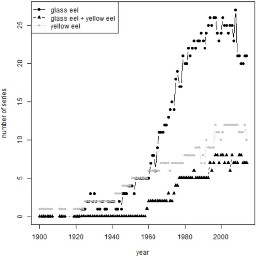
Figure 2.1. Location of the eel recruitment monitoring sites in Europe, circle = glass eel (white), glass eel and young yellow eels (blue), yellow diamond = yellow eel series. The lines show the different Eel Management Units in Europe.

The glass eel recruitment series have also been classified according to two areas: North Sea and Elsewhere Europe, as it cannot be ruled out that the recruitment to the two areas have different trends (ICES, 2010b). The Baltic area does not contain any pure glass eel series. The yellow eel recruitment series are either comprised of a mixture of glass eel and young yellow eel, or as in the Baltic, of young yellow eel only.

The WGEEL has collated information on recruitment in 52 time-series. The series code, name, comments about the data collection method, the international region, whether they are part of the North Sea or Elsewhere series, the country, EMU, river, location, sampling type, data units, life stages sampled, first and last year of data, whether they are active in the year of assessment, and whether or not there are missing data in the series, are all fully described in electronic Table E2.1 available on the working group web page.

Some series date back as far as 1920 (glass eel, Loire, France) and even to the beginning of 20th century (yellow eel, Gota Alv, Sweden). The status of the series can be described as following:

• 38 time-series were updated to 2014 (29 for glass eel or glass + yellow, and nine for yellow eel (Table 2.1).

• three series (one for glass eel and two for yellow eel) have been updated to 2013 only (Table 2.2).

• Some of the series have been stopped, as the consequence of a lack of recruits in the case of the fishery-based surveys (Ems in Germany, 2001; Vidaa in

(18)

Denmark, 1990), as a consequence of a lack of financial support (the Tiber in Italy, 2006), or from 2008 to 2011, as a consequence of the introduction of a new quota system and incomplete geographical reporting for the five fish-ery based French series (Table 2.3).

The number of available series has declined from a peak of 33 series in 2008 for the glass eel, and glass eel and young yellow eel series. The maximum number of yellow eel series increased to 12 in 2009 (Figure 2.2). Before 1960, the number of glass eel or glass eel + yellow eel series, which will be used to build the WGEEL recruitment index for glass eel, is quite small, with six series before 1959 (Figure 2.2). Those are Den Oever (scientific survey), the Loire (total catch), the Ems (mixture of catch and trap and transport), the Gironde (total catch), the Albufera de Valencia in the Mediterranean, and the Adour, which dates as far back as 1928, and is based on cpue. For the latter however, only the years 1928 to 1931 are available and the series only resumes in 1966.

Figure 2.2. Trend in number of series giving a report any specific year, data split per life stage. 2.1.2 Simple geometric means

The calculation of the geometric mean of all series show that the recruitment is increas-ing in 2014 from a minimum in 2009 (Figures 2.3 and 2.4). Figure 2.3, although con-sistent with the trend provided by WGEEL since 2002, might be biased by the loss of most Bay of Biscay series from 2008 to 2012. The scaling is performed on the 1979–1994 average of each series, and seven series without data during that period are excluded

(19)

from the analysis1_{. This scaling is simply to standardise the series so that they can all} be presented on the same y-axis, and this period of years is not presented as a reference time period.

Figure 2.3. Time-series of glass eel and yellow eel recruitment in European rivers with dataseries having data for the 1979–1994 period (45 sites). Each series has been scaled to its 1979–1994 average, for illustrative purposes. Note the logarithmic scale on the y-axis. The mean values and their boot-strap confidence interval (95%) are represented as black dots and bars. Geometric means are pre-sented in red. The shaded values correspond to pre-1960 where the number of glass eel dataseries available is lower and will not be included in the calculation of the reference period.

When looking at the separate trends for both glass eel and yellow eel series, as intro-duced by the WGEEL in 2006 (ICES, 2006), the increase seems mostly due to glass eel series which show a positive trend from 2011 while yellow eel series show a wider variation, and a large surge in 2014, that remains to be confirmed. Note that no lag was added to the yellow eel series but that the age of yellow eels might range from one to several years old (Figure2.4).

Following the recommendation of RGEEL (ICES, 2013b: Minutes of the Technical Re-view), in 2014 the same figure is built from all series available, and a new scaling based on the 2000–2010 (included) was performed. This leaves out two series: Vida and YFS1. The scale from this graph shows an increase from the current level (1) to around a 100

11the series left out are : Bres, Fre, Inag, Klit, Maig, Nors, Sle.

(20)

times that value in the 1970s, and more than 100 times that level before the 1970s for the longest series (Figure2.5).

Figure 2.4. Time-series of glass eel and yellow eel recruitment in Europe with 45 series out of 52 available to the working group. Each series has been scaled to its 1979–1994 average. The mean values of combined yellow and glass eel series and their bootstrap confidence interval (95%) are represented as black dots and bars2_{. The brown line represents the mean value for yellow eel, the}

blue line represents the mean value for glass eel series. The range of the series is indicated by a grey shade. The time period 1900–1950 that will not be used to calculate the reference is shaded in white. Note that individual series from Figure4.3 were removed for clarity. Note also the logarith-mic scale on the y-axis.

2 This is the same as in Figure 4.3.

(21)

Figure 2.5. Time-series of glass eel and yellow eel recruitment in Europe. Same graph as Figure 4.4 but the series have been scaled to their 2000–2009 average (blue box). Two series3_{have been}

ex-cluded from the initial number (52) that did not have data in the period 2000–2009. The mean values of combined yellow and glass eel series and their bootstrap confidence interval (95%) are repre-sented as black dots and bars. The brown line represents the mean value for yellow eel, the blue line represents the mean value for glass eel series. The range of the series is indicated by a grey shade. Note the logarithmic scale on the y-axis.

2.1.3 GLM based trend

The WGEEL recruitment index is a reconstructed prediction using a simple GLM (Gen-eralised Linear Model):glass eel ~ year : area + site, where glass eel is individual glass eel series, site is the site monitored for recruitment and area is either the North Sea or Elsewhere Europe. The GLM uses a gamma distribution and a log link. The dataseries comprising only glass eel, or a mixture of glass eel and what is mostly young of the year eel are grouped and later labelled glass eel series.

In the case of yellow eel series, only one estimate is provided: yellow eel ~ year + site. The trend is reconstructed using the predictions from 1960 for 40 glass eel series and for 12 yellow eel series. This analysis rebuilds all the series by extrapolating the missing values. The series are then averaged. Some zero values have been excluded from the GLM analysis: 12 for the glass eel model and one for the yellow eel model (see Table E2-1).

3 Vidaa and YFS1.

(22)

The reference period for pre-1980 recruitment level is 1960–1979, as four series availa-ble from 1950 to 1960 are excluded because they were based on total catch of commer-cial glass eel, which are known to have been affected by changes in fishing practises, and the progressive shift from hand nets to push net fisheries from 1940 to 1960 (Briand

et al., 2008: see paragraph 24.1.1). After 1960, the number of available series increases rapidly (Figure 2.2). Though no such biases are known for the yellow series recruitment series, the same reference period has been chosen, to provide consistent results. After high levels in the late 1970s, there has been a rapid decrease in the glass eel re-cruitment trends (Figures 2.6 and 2.7; note the logarithmic scales).

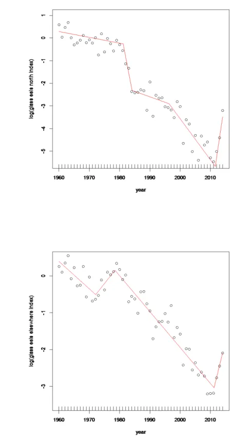
Figure 2.6. WGEEL recruitment index: mean of estimated (GLM) glass eel recruitment for the con-tinental North Sea and elsewhere in Europe updated to 2014. The GLM (recruit = area: year + site) was fitted on 40 series comprising either pure glass eel or a mixture of glass eels and yellow eels and scaled to the 1960–1979 average. No series are available for glass eel in the Baltic area. Note the logarithmic scale on the y-axis.

12.2

(23)

Figure 2.7. Mean of estimated (GLM) yellow eel recruitment and smoothed trends for Europe up-dated to 2014. The GLM (recruit ~ year + site) was fitted to 12 yellow eel series and scaled to the 1960–1979 average. Note the logarithmic scale on the y-axis.

In conclusion, the WGEEL recruitment index is currently low but increasing for both regional glass eel series: the current level with respect to 1960–1979 averages is 3.7% for the North Sea and 12.2% elsewhere in the distribution area (Tables 2.4 and 2.5).For yellow eel recruitment series, the recruitment has risen to 36% of the 1960–1979 period. 2.1.4 Are there significant changes in trend?

Given these recent increases in recruitment indices, the working group examined three statistical methods to test whether these were significant changes to the trends (i.e. break points, upturns). The objective of the first two methods, CUSUM and segmented regression, was to identify breakpoints in the whole time-series. The third method, the Bayesian approach, was used to detect a breakpoint in the last ten years and to simulate future recruitment to explore a trajectory of recruitment recovery

2.1.4.1 CUSUM

Trends were calculated using the cumulative sums method (CUSUM (Woodward and Goldsmith 1964; Ibanez et al., 1993). A cumulative sum represents the running total of the deviations of the first observation from a mean based on the same interval. In gen-eral, the CUSUM approach to detect change points performs well, has been well-doc-umented and is relatively easy to implement (Breaker, 2007). Breakpoints that may not

(24)

be possible to detect in the original data often become easier to detect when the CUSUM is plotted. For a time-series with data sampled for each year (t), a reference value k is chosen (here we chose the standardized mean logarithmic of the glass and yellow eel time-series).

After subtracting k from each datapoint, the residuals are added successively to calcu-late the cumulative sums (CSt):

𝐶𝐶𝐶𝐶𝑡𝑡=�(𝑥𝑥𝑖𝑖− 𝑘𝑘) 𝑡𝑡

𝑖𝑖=1

The successive values of CSt are plotted versus time (years) to produce the so-called CUSUM chart. The local mean between two breaking points is the slope of the cumu-lative sum curve between the two points, plus the reference value k. Changes in the average level of the process are reflected as changes in the slope of the CUSUM plot. For successive values equal to k, the slope will be horizontal; for successive values lower than k, the slope will be negative and proportional; and for successive values higher than k, the slope will be positive and proportional. The year of the change in the slope of the CUSUM is the year that a shift occurs. Breakpoints were visually identified on the CUSUM trajectories as abrupt changes (as opposed to a gradual change) in di-rection of slope.

CUSUM were first calculated on the whole time period (from 1960 to 2014) to define the main breakpoints (Table 2.6). Since two main periods were defined, CUSUM were then calculated on the second period, from 1980 onwards, to focus on the decline (Table 2.6).

All of the CUSUM calculated showed smooth trajectories with few breakpoints (Fig-ures 2.8 and 2.9). This was due to the low amplitude in inter-annual fluctuations com-pared to the overall change around the total average of the time-series.

Figure 2.8. CUSUM calculated on the original glass eel time-series (‘North Sea’ and ‘Elsewhere Eu-rope’), with CUSUM values plotted against the y-axis and year shown on the x-axis.

-2 0 2 4 6 8 10 12 14 1950 1960 1970 1980 1990 2000 2010 2020 CSM north CSM elsewhere

(25)

Figure 2.9. CUSUMS calculated on the natural logarithm of glass eel time-series (‘North Sea’ and ‘Elsewhere Europe’), from 1980 to 2014, with CUSUM values plotted against the y-axis and year shown on the x-axis.

The blue lines on Figures 2.10 and 2.11 show two distinct periods with breakpoints in 1980 for the ‘North Sea’ series and two years later for the ‘Elsewhere Europe’ time-series. The slopes of the CUSUM become negative after these breakpoints. While the time trend for ‘North Sea’ time-series only shows one breakpoint, the trend for ‘Else-where Europe’ time-series displays three breakpoints with a relatively stable period between 1982 and 1990 (Figure 2.11). CUSUM calculated over the later period (starting in 1980) show two breakpoints for the ‘North Sea’ time-series and one for the ‘Else-where Europe’ time-series (Figures 2.10 and 2.11).

-5 0 5 10 15 20 19 78 19 80 19 82 19 84 19 86 19 88 19 90 19 92 19 94 19 96 19 98 20 00 20 02 20 04 20 06 20 08 20 10 20 12 20 14 20 16 ln cusum north ln cusum elsewhere

(26)

Figure 2.10. Step diagram representing the slopes calculated on the logarithm of the different time-series for ‘North Sea’ and ‘Elsewhere Europe’ time-time-series, (see Table 2.6 for details on k), with slope values plotted against the y-axis and year shown on the x-axis.

Figure 2.11. Step diagram representing the slopes calculated on the logarithm of the different time-series, for ‘North Sea’ and ‘Elsewhere Europe’ time-time-series, after the decline in recruitment (see Ta-ble 2.6 for details on k), with slope values plotted against the y-axis and year shown on the x-axis. 2.1.4.2 Segmented regression

The R package “segmented” was used to perform the segmented regression (Muggeo, 2003; 2008). This algorithm estimates the positions of a given number of breakpoints, starting from a user-defined initial condition (i.e. breakpoints locations), by iteratively fitting linear segmented models with the following predictor:

-40

-35

-30

-25

-20

-15

-10

-5

0

19

60

19

63

19

66

19

69

19

72

19

75

19

78

19

81

19

84

19

87

19

90

19

93

19

96

19

99

20

02

20

05

20

08

20

11

20

14 north

elsewhere

-0.4 -0.2 0 0.2 0.4 0.6 0.8 1 1.2 1.4 19 80 1982 1984 1986 8819 1990 1992 1994 1996 1998 2000 2002 2004 0620 2008 2010 2012 2014 north elsewhere

(27)

𝛽𝛽1𝑧𝑧𝑖𝑖+𝛽𝛽2(𝑧𝑧𝑖𝑖− 𝜓𝜓)+

(𝑧𝑧𝑖𝑖− 𝜓𝜓)+= (𝑧𝑧𝑖𝑖− 𝜓𝜓) ×𝐼𝐼(𝑧𝑧𝑖𝑖>𝜓𝜓)

where 𝛽𝛽1 is the left slope, 𝑧𝑧𝑖𝑖 is the independent variable, 𝛽𝛽2 is the difference-in-slope

before and after a breakpoint, 𝜓𝜓 is the breakpoint and 𝐼𝐼(∙) is the indicator function, equal to one when the argument is true, otherwise it is zero.

This model is strongly affected by the initial conditions for the breakpoints locations and it is not intended to determine the number of breakpoints in a time-series. There-fore, this algorithm is nested into a double loop: the first to compare the null model (i.e. the linear regression with no breakpoints) and different segmented models with j

breakpoints (j= 1…4) and the second to compare several initial conditions, sampled

randomly from all the combinations of j possible breakpoints locations (here the sub-sample is the 10% of all possible combinations). The Bayesian Information Criteria (BIC) is used to determine the performance of each resulting model. BIC was preferred to the Akaike Information Criteria (AIC) as it has a higher penalty on the number of parameters. The model associated with the lowest value of BIC is selected.

This method has been applied to the three time-series: the logarithm of glass eels re-cruiting in the ‘North Sea’ area (north), the logarithm of glass eels rere-cruiting in the ‘Elsewhere Europe’ area (elsewhere) and the logarithm of yellow eels (yellow). The results are summarized in Table 2.7 and Figures 2.12 to 2.14.

(28)

a)

b)

Figure 2.12. Segmented regression performed on the log of glass eel recruitment at the ‘North Sea’ (a) and on the log of glass eel recruitment ‘Elsewhere Europe’ time-series (b).

(29)

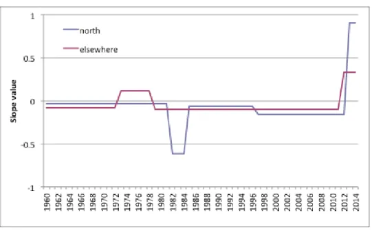
The calibration of the segmented regression model on the ‘North Sea’ time-series se-lected the model with four breakpoints (1981, 1984, 1996 and 2012) (Figure 2.12a). The 1981, 1984 and 1996 are breakpoints between regressions with negative slope, while the 2012 breakpoint identifies a change in the sign of the slope, from negative to posi-tive (Figure 2.13).

The model selected in the ‘Elsewhere Europe’ time-series identified three breakpoints (1972, 1978 and 2011), subdividing the time-series into four different periods with dif-ferent slopes (Figure 2.12b) that change sign at each breakpoint (Figure 2.13).

Figure 2.13. Step diagram representing the slopes calculated using the segmented regression model on the two recruitment time-series (‘North Sea’ and ‘Elsewhere Europe’).

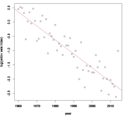
No breakpoints were identified for the yellow eel time-series and the null model was selected (Figure 2.14). This regression showed a significant (p<0.001) negative slope (𝛽𝛽=-0.049).

(30)

Figure 2.14. Segmented regression performed on the log of the yellow eel time-series.

The significance of using 2011 as a breakpoint in the recruitment time-series was tested using the model developed by SGIPEE (ICES, 2011b):

𝑅𝑅~𝑦𝑦𝑦𝑦𝑦𝑦𝑦𝑦+𝑝𝑝𝑝𝑝𝑦𝑦𝑥𝑥(𝑦𝑦𝑦𝑦𝑦𝑦𝑦𝑦, 2011)

Where 𝑝𝑝𝑝𝑝𝑦𝑦𝑥𝑥 is the maximum between the year and 2011. This model was calibrated on both recruitment time-series. An Analysis of Variance (ANOVA) revealed that the term pmax(.) was significantly different from zero (p<0.001 for both ‘North Sea’ and ‘Elsewhere Europe’).

2.1.4.3 Bayesian approach

The Bayesian Eel Recruitment Trend (BERT) model is based on exponential trends ( and ) and auto-correlated perturbations . This type of perturbation structure sim-ulates whether recruitment above the central trend in a particular year is more often followed by recruitment above or below the trend. This is the usual way to incorporate environmental fluctuations (e.g. climate, oceanic conditions) which are generally auto-correlated in time. This approach was adapted from that developed to set up the glass eel quota in France (Beaulaton et al., in press.)

The possibility of a single regime shift was introduced with an indicator random vari-able to test the credibility of this break point (Kuo and Mallick, 1998). The posterior distribution of can be interpreted as the probability that a shift in the trend should be included in the model. The shift occurs at which was chosen between 2003 and 2014, according to categorical distribution.

1

a

2

a

ε

_t

I

shift

t

(31)

The model is writte as:

where the recruitment index the year , the year of the regime shift, the slope before the regime shift, the slope after the regime shift, the indicator random variable to select or not the regime shift, the auto-correlated perturbations, the auto correlation coefficient and the independent and identically distributed residuals of mean 0 and standard deviation . is drawn from a Bernoulli distribu-tion of probability . is drawn from a categorical distribution with a 10 values probability vector of 0.1.

The a priori distributions are chosen as least informative.

where dunif, dgamma, dnorm and dbata are the density functions respectively for uni-form, gamma normal and beta distributions in jags.

Bayesian inferences were performed by Markov Chain Monte Carlo from the R pack-age ‘rjags’ (Plummer, 2013).

The recruitment time-series ‘Elsewhere Europe’ and ‘North Sea’ over the period 1980 to 2013 were used to target the analysis on breakpoints in the recent period. The refer-ence recruitment corresponds to the average recruitment during the referrefer-ence period 1960–1973 (Chapter 2.1). This reference recruitment was used as a proxy for the stock recovery.

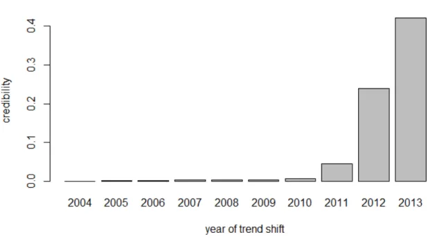
For the ‘Elsewhere Europe’ series, the BERT model gives a credibility of 35.1% for a trend shift between 2004 and 2013. The distribution of years with breakpoints is pre-sented in Figure 2.15. Note that the special case with and is the equivalent Bayesian approach of the test proposed by SGIPEE (ICES, 2011b). In that case, the credibility of a trend shift in 2011 is 72.3%. This result shows the importance of taking account of autocorrelation in the analysis for such trends.

( )

(

)

(

)

1 2 1 t-1 t-1 1

for

t

for

t

0 dcat rep 0.1,10

t t a shift t a I a shift t t t iid t I shift

R

e

t

R =

R

e

t

=

ρ

η

η Norm ,σ

I

Bernoulli p

t

ε ε

ε

+ + ⋅ + −



_⋅

_≤





⋅

<



⋅

+



t

R

_t

t

_shift

a

₁ 1 2

a

+

a

_I

t

ε

ρ

η

t

σ

I

p

t

_shift

(

)

(

)

(

)

( )

(

)

(

)

1 2 0

dunif

1,1

dgamma 0.01,0.01

,

dnorm 0, 0.01

log

dnorm 0, 0.01

dnorm(0, 1)

p

_I

dbeta 0.5, 0.5

a a

R

ρ

σ

−

+



0 ρ

=

t

_shift

=

2011

(32)

For the ‘North Sea’ series, with the full model, the credibility of a regime shift increased to 73.7% with the more likely breakpoint in 2013 (Figure 2.16).

Figure 2.15. Credibility of (equivalent in classical statistics to “the probability to have”) a trend shift according to year for the “Elsewhere Europe” time-series.

Figure 2.16. Credibility of (equivalent in classical statistics to “the probability to have”) a trend shift according to year for the “North Sea” series.

(33)

2.1.4.4 Conclusion on the break points detected

All methods applied on the complete time-series (1960–2014) detected a breakpoint around 1980, indicating a change in the slope sign from positive to negative, except the segmented regression on the glass eel recruitment in the ‘North Sea’ for which the breakpoint corresponded to an increased negative slope. This result confirms the shift in trend observed in the recruitment series during the 1980s and the consequent decline of the recruitment until the most recent years.

The models detected several other breakpoints that occurred before 2010. These break-points were not related to a change in the trend but to steeper declines in recruitment. Most models (except the CUSUM applied to the glass eel recruitment in the ‘Elsewhere Europe’ series) detected a breakpoint in 2011–2012 with a change of slope sign. The significance of this breakpoint was confirmed by the ANOVA and by the Bayesian ap-proach, but it was not possible to determine whether this breakpoint can be considered a trend shift yet, as this short positive trend could be the result of the time–series auto-correlation. Moreover, there is no evidence of a trend change in the yellow eel time– series.

2.1.4.5 Evaluation of recruitment recovery based on trend analysis

This objective of this section is to determine whether or not trends in recruitment are moving towards recovery.

It is obvious that a decreasing trend in recruitment is not compatible with recovery of the stock. An increase in recruitment, confirmed by lagged increases of the standing stock and silver eel escapement (when data will be available) is a necessary condition to consider a recovery. However a short-term increase will not necessarily certify re-covery. At least, an increase over a period that corresponds to the average lifespan should be recorded before giving a positive answer to recovery. Since life traits and contributions to spawning stock vary geographically, the definition of the average lifespan for eel is not simple and more work is needed.

Another way to evaluate whether the trend is moving towards recovery is to calculate how long it will take, given the present trend, to reach recruitment reference. In this analysis the recruitment reference is defined as the average recruitment observed dur-ing the period from 1960 to 1979.

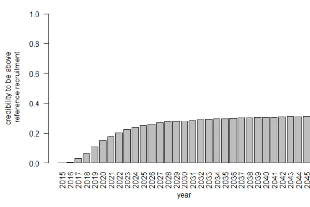
The projections of the recruitment are presented in Figures 2.17 and 2.18 for ‘Elsewhere Europe’ and ‘North Sea’ respectively. Since a trend shift is considered in only 35.1% of the cases for the ‘Elsewhere Europe’ series, the trend of recruitment is predicted to slightly decrease in the next years and the credibility (akin to statistical ‘probability’) to be above the reference recruitment does not exceed 35% in the next 30 years (Figure 2.19). For the “North Sea” series, the trend is increasing (Figure 2.18) but will only reach the reference recruitment in the long term (Figure 2.20).

(34)

Figure 2.17. Evolution from 1980 to 2014 (point) and projection from 2015 to 2030 (box and whiskers plot) of recruitment for ‘Elsewhere Europe’ time-series. In the box and whiskers plot, the horizontal segment in bold represents the median, the box represents the inter-quartile range, and the whisk-ers represent the extreme values.

Figure 2.18. Evolution from 1980 to 2014 (point) and projection from 2015 to 2030 (box and whiskers

plot) of recruitment for the ‘North Sea’ time-series. In the box and whiskers plot, the horizontal segment in bold represents the median, the box represents the inter-quartile range, and the whisk-ers represent the extreme values.

(35)

Figure 2.19. Evolution of the credibility (equivalent in classical statistics to the ‘probability’) to be above the reference recruitment (1960–1979 average recruitment) for the ‘Elsewhere Europe’ time-series.

Figure 2.20. Evolution of the credibility (equivalent in classical statistics to the ‘probability’) to be

(36)

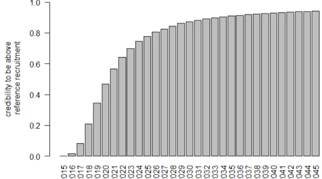
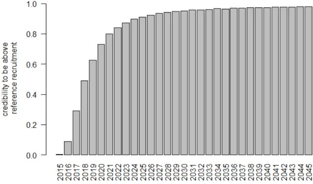
If a trend shift is set between 2004 and 2013 (i.e. assuming that the recent increases in recruitment trend continue in the future), the credibility to exceed the reference recruit-ment will be around 50% for ‘Elsewhere Europe’ in 2021, and for ‘North Sea’ in 2018, and higher than 95% after 2045 for ‘Elsewhere Europe’ and after 2029 for ‘North Sea’ recruitment (Figures 2.21 and 2.22).

Figure 2.21. Evolution of the credibility (equivalent in classical statistics to the ‘probability’) to be above the reference recruitment (1960–1979 average recruitment) for ‘Elsewhere Europe’ assuming a trend shift set between 2004 and 2013.

(37)

Figure 2.22. Evolution of the credibility (equivalent in classical statistics to the ‘probability’) to be above the reference recruitment (1960–1979 average recruitment) for the ‘North Sea’ time-series as-suming a trend shift set between 2004 and 2013.

In conclusion, the recent increases in recruitment time-series observed over the last three years are not sufficient to be sure that the stock is moving towards a recovery. If these positive trends are confirmed and continue in the future without any changes, the recruitment might be expected to exceed the average 1960–1979 level around the year 2030 in ‘North Sea’ and around the year 2045 in the ‘Elsewhere Europe’ times-series. However, much improved understanding of the functioning of the stock is re-quired to make these trend analyses more robust.

2.1.4.6 Indicators that might trigger an update assessment

The working group considered the question posed by the ICES Generic ToRs, to define or propose indicators that could be used to decide when an update assessment is re-quired.

First and foremost, the working group reiterated that the ‘3B and ΣA’ stock indicators should be estimated on an annual basis, and for each individual EMU, in order to up-date the precautionary diagram approach. It is also essential that the glass eel and yel-low eel data used to build recruitment and standing stock indices are collected annually.

Regarding indicators to trigger an update assessment, the working group proposed that a regime shift (change of sign in the trend) in recruitment time-series that was detected with a high probability in the recent past might be a suitable trigger for an update assessment. It that case, explanations of this regime shift should be explored. Biological processes of the population dynamics and possibly the biological reference points should be re-evaluated in consequence. Specific work is clearly required to de-fine more precisely such quantitative indicators for an update assessment.

(38)

2.2 Time-series of yellow and silver eel abundance

In addition to the glass eel and (young) yellow eel recruitment series, yellow eel and silver eel indices may be used in the future, though data are scarce, and may be uncer-tain. Moreover, yellow and silver eel data may be more representative for the local area where they are collected than for the global stock status because of the contrasts in population dynamics and anthropogenic pressures at the distribution area scale. Several Country Reports present information on long-term monitoring of yellow eel abundance in various habitats, and these values have been updated in the WGEEL da-tabase. Descriptions of the time-series are presented in Table 2.8. Methodologies vary from electrofishing and traps in rivers to beach-seines, fykenets and trawls in larger waterbodies.

Information on long-term changes in yellow eel abundance in many cases is the only way to assess the status of eel production in the absence of a significant fishery. A de-velopment towards standardized methods was suggested by WKESDCF to be in-cluded in the revisions to the DCF (ICES 2012a).

2.3 Commercial fishery landings trends

At the present 2014 status, dataseries presented in this report contains information ob-tained from the Country Reports, FAO capture database and by personal communica-tion from WGEEL participants (Table E2-2).

A review of the catches and landing reports in the Country Reports showed a great heterogeneity in landings data. Some countries make reference to an official system, which then reports either total landings or landings split by Management Unit or Re-gion. Some countries do not have any centralized system. Furthermore, some countries have revised their dataseries, with extrapolations to the whole time-series, during the process of compiling their Eel Management Plan (i.e. Poland, Portugal).

Landings data sourced from the FAO database are presented for countries not report-ing to WGEEL. These are the Mediterranean countries: Egypt, Tunisia, Morocco, Tur-key and Albania. The quality of some of the Mediterranean data should be reviewed, as some figures seems to be unreliable, e.g. 2012 Egypt data show large variations that were of uncertain provenance given that there was uncertainties about the presence of a catch reporting system.

2.3.1.1 Collection of landings statistics by country (from CRs)

Changes in following the descriptions of the landing statistics per country compared to 2013 WGEEL are highlighted in italics.

Norway: Provided official landing statistics (Fisheries Directorate) calculated

accord-ing to the number of licences. Fishaccord-ing for eel has been banned in Norway since January 1, 2010.

Sweden: Data on eel landings in coastal areas are based on sales notes sent to the

ap-propriate agency and in recent years also from a logbook system. There is a discrep-ancy between the data derived from the traditional sales notes system and the more recent logbook system. During the most recent years this difference was considerable, e.g. in 2011 sales notes reported 238 tonnes, whereas the logbooks system registered 355 tonnes (all from the marine areas). Landings data from freshwaters come from a

JOINT EIFAAC/ICES/GFCM WGEEL REPORT 2014

2014

ICES

A

C

ICES

CM

2014/ACOM:18

R

.

ACOM,

WGRECORDS,

SSGEF,

FAO,

EIFAAC

&

GFCM

Report of the Joint EIFAAC/ICES/GFCM

Working Group on Eel

3–7 November 2014

Rome, Italy

International Council for the Exploration of the Sea

Conseil International pour l’Exploration de la Mer

Contents

Executive summary

1

Introduction

2

ToR a): Assess the latest trends in recruitment, stock and

fisher-ies, including effort, and other anthropogenic factors indicative

of the status of the stock, and report on the state of the

inter-national stock and its mortality

-40

-35

-30

-25

-20

-15

-10

-5

0

19

60

19

63

19

66

19

69

19

72

19

75

19

78

19

81

19

84

19

87

19

90

19

93

19

96

19

99

20

02

20

05

20

08

20

11

20

14

north

_⋅

_≤

_t

_I