Scalable Software-Defect Localisation
by Hierarchical Mining of Dynamic Call Graphs
Frank Eichinger
∗Christopher Oßner
∗Klemens B¨
ohm
∗Abstract
The localisation of defects in computer programmes is essential in software engineering and is important in domain-specific data mining. Existing techniques which build on call-graph mining localise defects well, but do not scale for large software projects. This paper presents a hierarchical approach with good scalability characteristics. It makes use of novel call-graph representations, frequent subgraph mining and feature selection. It first analyses call graphs of a coarse granularity, before it zooms-in into more fine-grained graphs. We evaluate our approach with defects in the
Mozilla Rhino project: In our setup, it narrows down the code a developer has to examine to about 6% only. Keywords: applied data mining, call graphs, graph mining, scalability, software-defect localisation
1 Introduction
Software is rarely free from defects that cause failing behaviour. Manual debugging can be extremely expen-sive, and localising defects is the most time consuming and difficult activity in this context [5, 18]. Automated means to localise defects and to guide developers de-bugging a programme are more than desirable, for large software projects in particular. From a data mining perspective, Han and Gao identify software engineering and defect localisation in particular as a main area for domain-specific mining [14]. They point out that the integration of domain knowledge, i.e., specific data rep-resentations, as well as dedicated analysis techniques, are essential for the success of applied data mining.
One approach for defect localisation is to compare programme executions that are correct to executions that have failed. A variety of techniques has been proposed that mine dynamic call graphs, e.g., [4, 8, 11, 12, 21]. In such graphs, nodes typically represent methods and edges method invocations. See Figure 1(a) for an example. More specifically, the approaches try to identify patterns in programme executions that ∗Karlsruhe Institute of Technology (KIT), Germany. Email: {eichinger, ossner, klemens.boehm}@kit.edu
are typical for the failing case. Then they use these patterns to rank the methods being suspected to be defective. However, despite good results, the techniques proposed so far do not scale well with the size of the software project. This is caused by the NP-hard subgraph-isomorphism problem inherent to frequent subgraph mining. Various evaluations [4, 8, 11, 21] have demonstrated this effect: They deal with very small programmes such as theSiemens Programmes[16], with 200 to 700 lines of code (LOC).
Solving the scalability issues is challenging, as seem-ingly possible solutions have issues: (1) Using increased computing capabilities or distributed algorithms is not feasible due to exploding computational costs. We have experienced this effect in preliminary experiments as well. Further, spending a lot of computing time for graph mining might be inappropriate for defect locali-sation. (2) Solving the scalability issue with approxi-mate graph-mining algorithms might be a solution, but might miss patterns which are important for defect lo-calisation. For instance, [4] does not report any prob-lems caused by the well scaling LEAP algorithm [26], but does not analyse large programmes either.
A different starting point to deal with the scalabil-ity problem in call-graph-based defect localisation is the graph representation. We investigate graph representa-tions at coarser abstracrepresenta-tions than the method level, i.e., the package level and the class level, and we start at such a coarse abstraction beforezooming-in into a
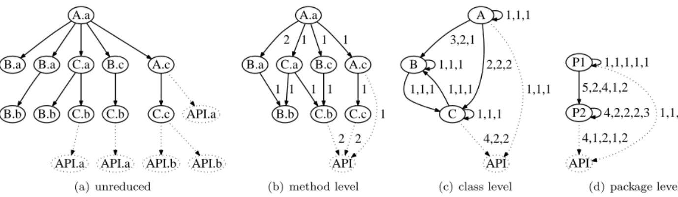
sus-a b c b b b (a) a b c b b ... b (b) a b 1 c 1 3 (c) Figure 1: (a) An unreduced call graph, (b) with a structure-affecting (dashed) and a frequency-affecting bug (dotted). (c) Thetotal reduction of (a) (weighted).
picious region of the call graphs. These graphs are a lot smaller than conventional call graphs, and they cause scalability problems in much fewer cases. However, this idea leads to new challenges:
1. Call-graph representations have not yet been stud-ied well for levels of abstraction higher than the method level. How do representations well-suited for defect localisation look like?
2. When zooming-in into defect-free regions by acci-dent: How to design hierarchical defect localisation in a way that minimises the amount of source code to be inspected by humans?
3. It is unclear which defects can indeed be localised in coarse graph representations.
Our approach for hierarchical defect localisation builds on the zoom-in idea and solves these challenges. This paper makes the following contributions:
Granularities of Call Graphs. We define call graphs at different levels of granularity, featuring edge-weight tuples that provide further information besides the graph structure (Challenge 1). We do so by taking the specifics of defect localisation into account: We explicitly consider API calls as well as inter-/intra-package and inter-/intra-class method calls.
Hierarchical Defect Localisation. We describe thezoom-in operationfor call graphs, present a method-ology for defect localisation for the graphs at each level and describehierarchical procedures for defect localisa-tion (Challenge 2). In concrete terms, we present dif-ferent variants of a depth-first search strategy to hier-archically mine a software project.
Evaluation with a Large Software Project. An essential part of our study is an evaluation featur-ing real programming defects in Mozilla Rhino (Chal-lenge 3). To this end we use the iBUGS repository [6] and the original test suite. Rhinoconsists of≈49k LOC, and the defects in the repository were obtained by join-ing information from a bug-trackjoin-ing system with data and source code from a revision-control system. To our knowledge, this paper is first to demonstrate the effec-tiveness of call-graph-mining-based defect localisation for large programmes and real defects. In our setup, the approach narrows down the amount of code a developer has to examine to about 6% of the whole project.
Identification of New Data-Mining Research Questions. This study has uncovered several new data-mining research questions. We discuss these ques-tions which might be relevant for many applicaques-tions.
Ideas related tozooming-ininto call graphs, namely Graph OLAP, have been described in [3]. The authors propose data-warehousing operations to analyse graphs, e.g., drill-down and roll-up operations, similar to our zoom-in proposal. However, [3] does not help in defect
localisation, as it aims at interactive analyses, and it does not consider specific requirements (e.g.,API calls). Paper organisation: Section 2 introduces founda-tions. Sections 3 and 4 explain call graphs and defect localisation based on them. Section 5 contains our eval-uation, Section 6 reviews related work, and Section 7 discusses threads of validity. Section 8 identifies chal-lenges for data-mining research, Section 9 concludes. 2 Foundations
In this section we introduce the notion of defects and the basics of call-graph-based defect localisation.
Defects in Software. In this paper, we distin-guish between defects, infections and failures [28]: De-fectsare the positions in the source code which cause an infection, aninfection is an incorrect programme state, andfailures are an observable incorrect programme be-haviour such as wrong calculation results. In our con-text, we use a further differentiation of ours [10]:
Occasional bugs are failures depending on the input data of the programme. Compared to non-occasional bugs, they are harder to localise since they require more test cases to be reproduced. Structure-affecting bugs are infections which affect the structure of a call graph. This is, when comparing graphs from correct and failing executions, certain graph substructures might or might not occur in either of the two variants. Figure 1(b) contains an example: a does not call b in case of an infection. There can be various reasons for this, e.g., a wrongly calculated variable value or a defective control statement, possibly within a. Call-frequency-affecting bugs are infections which change the call frequency of a certain substructure, rather than completely missing or adding structures. In Figure 1(b), the call frequency of
b fromc has changed, compared to Figure 1(a). We focus onoccasional bugs, as all call-graph-based defect-localisation approaches do. This requires that both correct and failing executions are available. With our approach, defects might bestructure affecting, call-frequency affecting, or both.
Defect Localisation with Call Graphs. A num-ber of call-graph-based techniques for defect localisation has been proposed [4, 8, 9, 11, 12, 21]. Their intuition is to mine for patterns in the call graphs which are charac-teristic for failing executions. Then they derive a defec-tiveness likelihood for each method. A method ranking based on such likelihoods can then guide the debugging process. The different proposals use differentcall-graph representations anddefect-localisation approaches. We now briefly review the most important differences.
Concerning the graph representations, the various approaches differ with regard to thelevel of granularity, the degree of reduction, and the questions if temporal
information is included and if the graphs areweighted. The first three aspects bear a trade-off between the size of the graphs and potentially more precise results on the one side and scalability on the other side.
Level of granularity: The graphs used in most ap-proaches [4, 8, 11, 12, 21] are method-level call graphs, i.e., nodes represent methods and edges method calls. (See Figure 1(a) for an example.) [4] presents a more fine-grained basic-block-level graph representation in addition to the method level. [9] is a preliminary study of ours investigating defect localisation with class-level call graphs. It aims at a scalable solution for large software projects. However, it does not investigate a comprehensive hierarchical approach. Degree of reduc-tion: In unreduced call graphs, as directly obtained from tracing, a method typically occurs several times, at various positions within a graph (see Figure 1(a)). [4, 9, 12, 21] build on call graphs where exactly one node represents a method (total reduction, see Figure 1(c)). [8, 11] in turn allow for more than one node. This promises more precise results, as more detailed contexts of method calls can be included in the analysis. How-ever, this leads to larger graphs; see [10]. Temporal information: The graphs in [4, 8, 21] incorporate tem-poral information, the ones in [9, 11, 12] do not. The experiments in [10] do not lead to any results that justify the increased graph size. Weighted graphs: In contrast to all other representations, the graphs in [9, 11, 12] are weighted. Edge weights represent the number of corre-sponding method calls (see Figure 1(c)), facilitating the localisation of call-frequency-affecting bugs.
Besides different call graph representations, the var-ious defect-localisation approaches localise defects in different ways. In concrete terms, they employ tech-niques as diverse assupport values,graph classification, discriminative subgraph mining and feature selection: [8] derives defect likelihoods fromsupport values of sub-graph patterns in call sub-graphs representing correct and failing programme executions. [21] builds ongraph clas-sification with subgraph patterns. The authors first mine frequent subgraph patterns before they use them to train a classifier. They then consider the difference in accuracy between two classifiers – one built with graph patterns including a certain method and one without them – as evidence for a defective method. [4] relies on discriminative subgraph mining. This technique finds subgraphs that discriminate well between correct and failing executions and thus directly identifies methods that are possibly defective. In [11], we make use of two kinds of evidence, support values and feature selection with edge weights. In [12], we target defects that affect the dataflow of a programme, by extending call graphs with abstractions referring to the dataflow.
The approaches mentioned do not scale for large software projects such as Mozilla Rhino. This paper in turn describes a scalable approach. It generalises previous work [9, 11], and it hierarchicallyzooms-ininto parts of call graphs deemed problematic.
3 Dynamic Call Graphs at Different Levels In this section, we propose and define totally-reduced call-graph representations for the method, class and package level (Sections 3.1–3.3). Then we introduce the zoom-in operation for call graphs (Section 3.4). Our graphs can easily be extended in either direction: More coarse-grainedmeta-package-level call graphs could rely on the hierarchical organisation of packages and would allow to analyse even larger projects. Graphs more detailed than the method level, e.g., at the level of basic blocks [4], would allow for a finer defect localisation.
On a technical level, we use AspectJ[19] to weave tracing functionality into Java programmes and to de-rive call graphs from programme executions. This yields an unreduced call-graph representation at the method level. (Figure 2(a) is an example.) This is the basis for all reduced representations we discuss in the follow-ing. In concrete terms, our tracing functionality inter-nally stores unreduced call graphs in a pre-aggregated space-efficient manner. This lets us derive call-graph representations at any levels of granularity.
3.1 Call Graphs at the Method Level. In this paper, we propose total graph reductions that are weighted, where exactly one node represents a method. We do not make use of any temporal information. All this leads to a compact graph representation [10].
As an innovation, we consider calls of methods belonging to theJavaclass library (API) in all graphs. We do so as we believe that some defects might affect the calls of such methods. To our knowledge, no previous study has considered such method calls. However, to keep the instrumentation overhead to a minimum, we do not considerAPI-internal method calls. In the graph representation, we use one node (API) to represent all methods belonging to the class library.
Notation 1. A method-level call graph is a graph where every method is represented by exactly one node, directed edges represent method invocations, and edge weights stand for the frequencies of the calls represented by the edges. The API node represents all methods of the class library and does not have any outgoing edges. Example. Figure 2(b) is a method-level call graph. It is the reduced version of the graph in Figure 2(a). The API nodes in Figure 2(a) represent twoAPI methods,
A.a
B.a B.a C.a B.c A.c
B.b B.b C.b C.b C.c API.a
API.a API.a API.b API.b
(a) unreduced A.a B.a 2 C.a 1 B.c 1 A.c 1 B.b 1 1 C.b 1 1 C.c 1 API 1 2 2 (b) method level A 1,1,1 B 3,2,1 C 2,2,2 API 1,1,1 1,1,1 1,1,1 1,1,1 1,1,1 4,2,2 (c) class level P1 1,1,1,1,1 P2 5,2,4,1,2 API 1,1,1,1,1 4,2,2,2,3 4,1,2,1,2 (d) package level Figure 2: An unreduced call graph and its total reduced representations at the method level, class level and package level. Notation: class.method; classAforms packageP1, classesB andC form packageP2.
3.2 Call Graphs at the Class Level. We now pro-pose class-level call graphs with tuples of weights. The rationale is to include some more information, which would otherwise be lost by the rigorous compression.
Notation 2. In class-level call graphs, every class is represented by exactly one node, and edges represent inter-class method calls (or intra-class calls in case of self-loops). The API node is as in the method-level call graphs. An edge is annotated with a tuple of weights: (t, u, v). t refers to the total number of method calls represented by the edge (as in method-level call graphs),
u is the number of different methods invoked, and v is the number of different methods that invoke methods. Example. Figure 2(c) is a class-level call graph, it is the compression of the graphs in Figures 2(a) and (b). Class-level call graphs may include self-loops (except for theAPI node), even if there is no recursion.
3.3 Call Graphs at the Package Level. The re-duction for this level is analogous to the previous ones, but to capture more information, we extend the edge-weight tuples by two elements:
Notation 3. In package-level call graphs, there is one node for each package, and there is an additional API node. The edge-weight tuples are as follows: (tm, uc, um, vc, vm), where uc is the number of different
classes called,vc the number of different classes calling,
and tm, um, vm are as t, u, v in Notation 2. (‘m’ stands
for method, ‘c’ for class.)
Example. We assume that class A in Figure 2 forms package P1, that classes B and C are in package P2, and that methodsAPI.aandAPI.bbelong to the same class. Figure 2(d) then is a package-level call graph, representing the call graphs from Figures 2(a)–(c).
3.4 The Zoom-In Operation for Call Graphs. Before we discuss thezoom-inoperation for call graphs, we first define an auxiliary function:
Definition 1. The generate function is of the fol-lowing type: generatelevel ∶ (Gunreduced,V) → Glevel,
where Gunreduced stands for unreduced call graphs,
Glevel for call graphs of the level specified by level ∈ {method,class,package} andVfor sets of vertices. A∈ V specifies the area to be included in the graph to be generated, by means of a set of vertices of the package level (package names) in case ‘level = class’ or of the class level (class names) in case ‘level = method ’. In case ‘level =package’, A= ☆selects all packages.
From a given unreduced graph, the function gen-erates a subgraph at the level specified, containing all nodes contained inA(all nodes ifA≠ ☆) and edges con-necting these nodes. If A= ☆, the function introduces a new node labelled ‘Dummy’ in the subgraph generated that stands for all nodes not selected byA.
In the generate function, we treat the API nodes separately from other nodes. They do not have to be explicitly contained in A, but are contained in the resulting graphs by default, as described in Notations 2 and 3. As the generate function selects certain areas of the graph, it obviously omits other areas. This is a conscious decision, as small graphs tend to make graph mining scalable. As calls of methods in the omitted areas might indicate defects nevertheless, the generate function introduces the Dummy nodes to keep some information about these methods.
Tozoom-in to a finer level of granularity, say into a certain packagep∈V(Gp)(V denotes the set of vertices of a graph) of a package-level call graphGpto obtain a class-level call graphGc, one calls thegenerate function as follows: Gc∶=generateclass(Gu,{p}), whereGuis the unreduced call graph ofGp. Zooming from a class-level call graph to a method-level call graph is analogous.
4 Hierarchical Defect Localisation
We now describe our hierarchical approach for defect localisation. At first, we introduce defect localisation without considering the hierarchical procedure, i.e., we describe how defect localisation works for call graphs at any selected level of granularity (Section 4.1). We then present different approaches for turning this technique into a hierarchical procedure (Section 4.2).
4.1 Defect Localisation in General. We now dis-cuss defect localisation with call graphs at arbitrary lev-els of granularity. After a short overview, we describe subgraph mining and defect localisation based on edge-weight tuples. Finally, we discuss the incorporation of information from static source-code analysis.
Overview. Algorithm 1 works with unreduced call graphs U, representing programme executions. More specifically, it deals with graphs at a user-defined level, describing a certain subgraph of the graphs (parame-ter A). For the time being, we consider the package level (A= ☆), i.e., without restricting the area. The al-gorithm first assigns aclass∈ {correct,failing}to every graph u∈U (Line 3), using a test oracle. Such oracles are typically available [18]. Then the procedure gener-ates reduced call graphs, from every graph u(Line 4). Next, the procedure derives frequent subgraphs of these graphs, which provide different contexts (Line 5). The last step calculates a likelihood of containing a defect, for every software entity eat the level specified (i.e., a package, class or method; Line 6). We do so by deriving a discriminativeness measure for the edge-weight-tuple values, in each context separately. TheP values for all entities of a certainlevel form a ranking of the entities, which can be given to software developers. They would then review the suspicious entities manually, starting with the one which is most likely to be defective. Alter-natively, this result can be the basis for a zoom-in into a finer level of granularity, as described in Section 4.2.
Algorithm 1Procedure of defect localisation. Input: a set of unreduced call graphsU,
alevel ∈ {package,class,method}, an areaA
Output: a ranking based on each software entity e’s likelihood to be defectiveP(e)
1: G= ∅// initialise a set of call graphs 2: for allgraphs u∈U do
3: check ifurefers to a correct execution, and assign aclass∈ {correct,failing}tou 4: G=G∪ {generatelevel(u, A)}
5: SG=frequent subgraph mining(G)
6: calculateP(e)for all software entitieseat thelevel specified, based onSG
Subgraph Mining. The frequent-subgraph-min-ing step (Line 5 in Algorithm 1) mines the pure graph structure and ignores the edge-weight tuples for the mo-ment. This is as conventional graph-mining algorithms do not take weights into account. Later steps will make use of them. We use the subgraphs obtained as differ-ent contexts and perform all further analyses for every subgraph context separately. This aims at a higher pre-cision than an analysis without such contexts and allows localising defects that only occur in a certain context. Example. A failure might occur when methodais called from method b, only when method c is called as well. Then, the defect might be localised only in the context of call graphs containing all methods mentioned, but not in graphs without method c.
We rely on the ParSeMiS implementation [24] of
CloseGraph [27] for frequent subgraph mining. Close-Graph has successfully been used in related studies [9, 11, 12, 21]. In a set of graphs G, it discovers subgraphs with a user-defined minimum support. For this value, we use min(∣Gcorr∣,∣Gfail∣)/2, where Gcorr and Gfail are the sets of call graphs of correct and failing executions, respectively (G = Gcorr∪Gfail). This ensures that no structure occurring in at least half of all executions be-longing to the smaller class is missed. Preliminary ex-periments have shown that this minimum support al-lows for both short runtimes and good results.
The API and Dummy nodes as well as self-loops (⤾) require a special treatment during subgraph mining. API nodes: As almost all methods call API methods, almost every node in a call graph has a con-nection to theAPI node. This increases the number of edges in a call graph significantly, compared to a graph without API nodes, possibly leading to scalability is-sues. At the same time, as almost every node has an edge to anAPI node, these edges usually are not inter-esting for defect localisation. We therefore omit these edges during graph mining, but keep the edge-weight tuples for the subsequent analysis step. This is, only nodes and edges drawn with solid lines in Figure 2 are considered. Dummy nodes: We treatDummy nodes in the same way as we treat API nodes, as their struc-tural analysis with subgraph mining does not seem to be promising. Dummy nodes tend to be connected to many other nodes as well, leading to unnecessarily large graphs. Self-loops: Such edges result from recursion at the method level. However, at the package and class level, a self-loop represents calls within the same entity, which happens frequently. Therefore, self-loops enlarge the graph significantly while not bearing much informa-tion. We therefore treat self-loops at the package and class level as API and Dummy nodes: We omit them
exec. sg1 sg2 ⋯ class AB AC A⤾ B⤾ C⤾ A API CAPI BC ⋯ (⤾,API) t u v t u v t u v t u v t u v t u v t u v t u v g1 3 2 1 2 2 2 1 1 1 1 1 1 1 1 1 1 1 1 4 2 2 1 1 1 ⋯ ⋯ correct ⋮ ⋮ ⋮ ⋮ ⋮ ⋮ ⋮ ⋮ ⋮ ⋮ ⋮ ⋮ ⋮ ⋮ ⋮ ⋮ ⋮ ⋮ ⋮ ⋮ ⋮ ⋮ ⋮ ⋮ ⋮ ⋱ ⋱ ⋮ gn 9 1 1 2 2 2 1 1 1 1 1 1 1 1 1 1 1 1 4 2 2 - - - ⋯ ⋯ failing
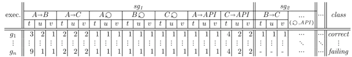
Table 1: Example feature table for class-level call graphs.
during graph mining and keep the edge-weight tuples for subsequent analysis.
Edge-Weight-Based Defect Localisation. When graph mining is completed, we calculate the likelihood that a method contains a defect (Line 6 in Algorithm 1). The rationale is to identify methods which call other methods with discriminative edge-weight-tuple values, i.e., method calls whose frequencies vary in correct and failing executions. As mentioned, we analyse every edge weight in the call graphs in the context of every subgraph mined. This aims at a high probability to reveal a defect, as every edge weight is typically investigated in many different contexts. To this end, we assemble a feature table as follows:
Notation 4. Afeature tablefor defect localisation has the following structure: The rows stand for all pro-gramme executions. For every edge in every frequent subgraph, there is one column for every edge-weight-tuple element (i.e., a single call frequency t or tuples of values, depending on the granularity level of the call graph considered, see Section 3). For all edges leading to API and Dummy nodes as well as for all self-loops (⤾), there are further columns for the edge-weight-tuple ele-ments; again, for each subgraph separately. The table cells contain the edge-weight-tuple values, except for the very last column, which contains the class ∈ {correct , failing}. If a subgraph is not contained in a call graph, the corresponding cells have a null value (‘-’).
We do not include Dummy nodes in the tables when considering the method level, as preliminary experiments have shown that this does not lead to any benefit. However, we includeAPI nodes at all levels. Example. Table 1 is a feature table corresponding to class-level call graphs, such as the one in Figure 2(c). (This graph is execution g1 in the table.) Suppose that the preceding graph-mining step has found two subgraphs, sg1 (B AC) and sg2 (BC). The very first column lists the call graphsg∈G. The next column corresponds to sg1 and edge AB with the total call
frequency t. The following two columns correspond to the remaining two edge-weight tuple elements u
and v (see Notation 2). Then follows the second edge in the same subgraph (AC) with its edge-weight
tuple(t, u, v). Next, all self-loops (A⤾,B⤾,C⤾) and API calls (AAPI,CAPI) insg1 are listed. (Dummy
nodes would be listed here as well, but do not exist in this example.) The same columns for subgraphsg2 and
finally the class of the execution follow. Graphgn does
not contain sg2, which is indicated by ‘-’.
After assembling the feature table, we em-ploy the information-gain feature-selection algorithm (InfoGain, [25]) in itsWekaimplementation [13] to cal-culate the discriminativeness of the columns and thus of the different edge-weight-tuple values. TheInfoGain is a measure from information theory and builds on en-tropy. Values ofInfoGainare in the interval[0,1]. High values indicate a table column affected by a defect. For this step, we could choose from various feature-selection algorithms available. However, previous work [11, 12] has shown that entropy-based measures are well-suited for defect localisation.
So far, we have derived defect likelihoods for every column in the table. However, we are interested in likelihoods for software entities (i.e., packages, classes or methods), and every software entity corresponds to more than one column in general. To obtain the defect likelihood P(e) of software entity e, we assign every column to the calling software entity. We then calculate P(e)as the maximum of theInfoGain values of the columns assigned to e. By doing so, we identify the defect likelihood of a software entity by its most suspicious invocation. The call context of a likely defective software entity and suspicious columns are supplementary information which we report to software developers to ease debugging.
Example. The graphsg1(see Figure 2) andgnin Table 1
display similar values, but refer to a correct and a failing execution. Suppose that method A.a contains a defect with the implications that (1) method B.c will not be called at all, and (2) that methodB.awill be called nine times instead of twice. This is reflected in columns 2–4, referring to (t, u, v) of AB in sg1. t increases from
three (1×B.c, 2×B.a) to nine (9×B.a),udecreases from two (B.c,B.a) to one (B.a), andv stays the same – in classA, only methodainvokes other methods. The InfoGain measure will recognise fluctuating values of t
Incorporation of Static Information. The edge-weight and InfoGain-based ranking procedure sometimes has the minor drawback that two or more en-tities (i.e., packages, classes or methods) have the same ranking position. In such cases, we fall back to a second ranking criterion: We sort such entities decreasingly by their size in (normalised) lines of code (LOC) derived withLOCC[17]. The rationale is that the size frequently correlates with the defectiveness likelihood [23]. This is, large methods tend to be more defective.
4.2 Hierarchical Procedures. The defect-localisa-tion procedure described in Secdefect-localisa-tion 4.1 can already guide a manual debugging process: A developer can first do defect localisation at the package level. She or he can then decide to zoom-in into certain suspi-cious packages. The developer would continue with our defect-localisation technique at the class level, proceed-ing with the method level etc. However, it might hap-pen that the developerzooms-in into an area where no defect is located. In this case, the developer would back-track and zoom-in elsewhere etc. This manual process, guided by our technique, bears the potential that im-portant background knowledge known to the developer can be easily included.
In this section, we say how to turn the manually-guided debugging process into semi-automatic proce-dures for defect localisation. We present a depth-first-search-based (DFS-based) procedure and a so-called merge-based variant. We also propose a technique that partitions large packages and classes.
DFS-Based Defect Localisation. Our DFS-based procedure follows the idea to manually investigate the most suspicious method in the most suspicious class in the most suspicious package first. If this first method turns out to not be defective, we go to the second most suspicious method in the same class. If all methods in this class are investigated, we backtrack to the next class etc. We further propose the parameters k, l, m. They limit the number of software entities to be investigated at each stage, to k packages, l classes and m meth-ods. Algorithm 2 formalises this approach. The param-eters k, l, m can be set to infinity in order to obtain a parameter-free algorithm; at the end of this section we also present a means to set these parameters.
Algorithm 2 iterates through three loops, one for packages, one for classes and one for methods (Lines 3, 6 and 9). In each loop, the algorithm calculates a defectiveness likelihood P for the respective software entities. This is, Lines 1–2, 4–5 and 7–8 comprise the graph-mining step (Line 5 in Algorithm 1) and the step that calculatesP (Line 6 in Algorithm 1), as described in Section 4.1. These lines make use of the generate
Algorithm 2DFS-Based Defect Localisation.
Input: a set of classified (correct, failing) unreduced call graphsU, parametersk, l, m
Output: a defectivemethod 1: SG=frequent subgraph mining(
{generatepackage(u,☆)∣u∈U}) 2: calculateP(package), based onSG 3: for allpackage∈topk(P(package)),
ordered decreasingly byP(package)do 4: SG=frequent subgraph mining(
{generateclass(u,{package})∣u∈U}) 5: calculateP(class), based onSG 6: for allclass∈topl(P(class)),
ordered decreasingly byP(class)do 7: SG=frequent subgraph mining(
{generatemethod(u,{class})∣u∈U}) 8: calculateP(method), based onSG 9: for allmethod ∈topm(P(method)),
ordered decreasingly byP(method)do 10: presentmethod to the user
11: if method is defectivethen
12: return method
function (see Definition 1), each with the area selection based on the currently selected software entity at the respective coarser level. Ultimately, the algorithm presents suspected methods to the user and terminates in case the user has identified a defect (Lines 10–12).
The DFS-based procedure described works interac-tively. This is, the potentially expensive graph-mining step as well as the calculation of P are done only when needed – the algorithm might terminate before all pack-ages and classes have been analysed. The suspected methods are presented to the user in an on-line manner. This avoids long runtimes before a developer actually can start debugging. However, it is of course possible to skip Lines 10–12 in Algorithm 2 and to save the current method to an ordered list of suspected methods. This leads to a ranking as described in Section 4.1. To ease experiments, we follow this approach in our evaluation. The proposed approach obviously has the drawback that the user has to set the parametersk, l, m. When the values are too low, the technique might miss a defect. Based on our experience, it is not hard to set appropri-ate parameters based on empirical values derived from debugging other defects in the same project. Further-more, we will present an automated choice of optimal parameter values in the following paragraphs.
Merge-Based Variant of DFS-Based Defect Localisation. This technique is an alternative to the DFS-based one. Instead of presenting the results to the user in an on-line manner, it replaces Lines 10–12 in
Algorithm 2 with code that saves all methods processed (along with their likelihood P) in a result set. Then, right after Line 12 in Algorithm 2, it sorts all methods decreasingly by their defect likelihood.
The drawback of this procedure is that the algo-rithm has to terminate before one can actually start debugging. On the other side, we hypothesise that the defect localisations obtained by this merge-based vari-ant are better than the ones with the first approach. We evaluate this hypothesis in Section 5.
Concerning the parametersk, l, m, the merge-based variant is more robust. As the merged result set is sorted at the very end, large parameter values usually do not lead to worse localisation results. They only affect the runtime. As yet another variant, we propose parameter-free defect localisation. Here we set the parametersk, l, mto infinity. This promises to not miss any defective method. In addition, if one uses this variant several times with a certain software project, one can use it to empirically set the parameter values. This allows for an efficient usage of the interactive (on-line) DFS-based procedure without parameters that are too high or to speed up the regular merge-based variant. Partitioning Approach. The hierarchical proce-dures investigated in this paper analyse smallzoomed-in call graphs at several granularities. However, a number of software projects – especially large ones and those with a long history – have imbalanced sizes of packages and classes. This might lead to large graphs that cause scalability issues, even if we are considering a zoomed-in subgraph only. It is an open research question how to overcome such situations. For now, we present a sampling-based partitioning approach for such cases.
Whenever a certain call graph at the package or class level is too large to be handled, we partition the graph into two (or, if needed more) partitions. We do so by randomly sampling nodes from the graph. We keep the edges connecting two nodes within the same partition. As not all edges connect nodes belonging to the same partition, we would lose a lot of information. To compensate for this effect, we introduce a dummy node Dummypart in each partition, representing all nodes in other partitions. We treat Dummypart nodes in exactly the same way asDummy nodes, i.e., we omit them during graph mining and include the edge-weight-tuple values in the feature tables.
When graph partitions are generated and Dummypart nodes are inserted, we do defect lo-calisation as described before with each partition separately. Then, similarly to the merge-based variant, we merge the rankings obtained from the different partitions and obtain a defectiveness ranking ordered by the P values of the software entities. This lets us
proceed with any manual or automated hierarchical defect localisation procedure, as described before.
This partitioning approach for large packages and classes has worked well in preliminary experiments. However, there might be cases where a loss of relevant information exists, and defect localisation might not work. For instance, think of a defect which occurs in a certain subgraph context that is distributed over several partitions. In such situations, the defect-localisation procedure can be repeated with a different partitioning, either based on the expertise of a software developer or by using another seed for random partitioning.
5 Evaluation with Real Software Defects We now evaluate our defect-localisation techniques in order to demonstrate their effectiveness and usefulness for large software projects. After a description of the target programme and the defects (Section 5.1) we explain the evaluation measures used (Section 5.2). Then we focus on defect localisation at the different levels in isolation (Section 5.3). Finally, we evaluate the hierarchical defect-localisation approaches (Section 5.4). 5.1 Target Programme and Defects: Rhino. For our evaluation we rely on Mozilla Rhino, as pub-lished in the iBUGS project [6]. Rhino is an open-source JavaScript interpreter, consisting of nine pack-ages, 146 classes and 1,561 methods or≈49k LOC (nor-malised 37k LOC).iBUGSprovides a number of original defects that were obtained by joining information from the bug-tracking system of the project with data and source code from its revision-control system. Further-more, it contains the original test cases along with the test oracles. See [7] for details on how the data was obtained. All in all, Rhino from the iBUGS repository provides a realistic test scenario for defect localisation in a large software project, at least compared to pro-grammes used in related evaluations that are two orders of magnitude smaller, e.g., [4, 8, 11, 21].
Concretely, we make use of 14 defects (Table 2 lists the defect numbers) from the iBUGS Rhino repository which have associated test cases and represent occa-sional bugs. These defects represent different real pro-gramming errors, and they are hard to localise: They occur occasionally and have been checked-in into the revision-control system before a failing behaviour has been discovered. See theiBUGSrepository [6] for more details. In addition, iBUGS provides about 1,200 test cases consisting of someJavaScriptcode to be executed byRhino, together with the corresponding oracles. As in many software projects, there are only a few failing test cases for each defect, besides a lot of passing cases. To obtain a sufficient number of failing cases, we have
gen-level/ defect 85880 114491 114493 137181 157509 159334 177314 179068 181654 181834 184107 185165 191668 194364 ∅ package 2 1 1 4 2 1 1 1 3 1 3 1 3 2 1.9 class 1 8 8 16 20 1 2 15 5 1 1 2 3 3 6.1 method 1 2 2 - 1 1 1 10 3 3 9 10 1 2 3.5
Table 2: Defect-ranking positions for the three levels separately.
erated new ones by varying existing ones. In concrete terms, we have mergedJavaScriptcode from correct and failing test cases.
5.2 Evaluation Measures. In order to assess the precision of our techniques, we consider the ranking po-sitions of the actual defects. These popo-sitions quantify the number of software entities (i.e., packages, classes and methods) a software developer has to investigate in order to find the defect. (Smaller numbers are pre-ferred.) As the sizes of methods can vary significantly, we deem it more adequate to assess the hierarchical approaches by considering the normalised LOC rather than only the number of methods involved. We there-fore provide the percentage of LOC to examine in addi-tion to the ranking posiaddi-tion. We calculate the percent-age as the ratio of methods that has to be examined in the software project, i.e., the sum of LOC of all meth-ods with a ranking position smaller than or equal to the position reported, divided by the total LOC.
5.3 Experimental Results (Different Levels). We now present the defect-localisation results for the three different levels. This is, we consider complete package-level call graphs and call graphs at the class and method level, zoomed-in into the correct package (and class). We do so in order to assess the defect-localisation abilities for every level in isolation.
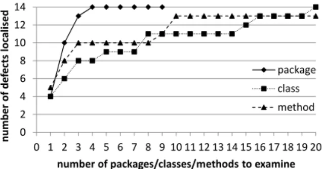
0 2 4 6 8 10 12 14 0 1 2 3 4 5 6 7 8 9 10 11 12 13 14 15 16 17 18 19 20 numbe r of de fe cts lo ca lis ed number of packages/classes/methods to examine package class method
Figure 3: The numbers of defects localised when exam-ining a certain number of packages/classes/methods.
Table 2 contains the experimental results, the rank-ing positions for all defects investigated, separately for the three levels. Figure 3 provides a graphical represen-tation of the same data. It plots the number of defects
localised when a developer examines a certain number of the top-ranked entities. For example, the third trian-gular point from the left means that 10 out of 14 defects are localised when examining up to three methods.
At thepackage level, the defective package is ranked at position one or two in 10 out of 14 cases, i.e., localisation is precise. The explanation for such good results at the coarsest level is the small number of nine packages in Rhino. At the class level, the results look a little worse at first sight. However, eight defects can be localised when examining three classes or less (out of 146). Only three defects are hard to localise, i.e., a developer has to inspect 15 or more classes. At the method level, 13 of the defects can be localised by examining 10 methods or less (out of 1,561), 10 of them with three methods or less. Only one defect, no. 137181, cannot be localised at all. This defect does not affect the call-graph structure nor the call frequencies.
All in all, the call-graph representations at the different levels – as well as the localisation technique – localise most defects with a high precision. However, when using package-level graphs to manually zoom-in into a package, packages ranked at position three or four might be misleading. This is not unexpected, as it is well known that many defects have effects only in their close neighbourhood [7]. This might not affect a package-level graph at all. The hierarchical approaches, in particular the merge-based ones, try to overcome this effect by investigating several packages systematically.
We use the results from this section to set the parameters k, l, mfor the hierarchical approaches. The maximum localisation precision in Figure 3 is reached at four packages, 20 classes or 10 methods. When using these values as parameters, the hierarchical approaches do not miss any defects they could actually localise while avoiding to examine more source code than necessary. 5.4 Experimental Results (Hierarchical). We now present the results from three experiments with the different hierarchical approaches (see Section 4.2): E1 – DFS-based defect localisation; E2 – merge-based variant thereof; E3 – parameter-free defect localisation. Table 3 contains the numerical results in two variants: the ranking positions at the method level and the corre-sponding percentage of source code. As before, Figure 4
exp./ defect 85880 114491 114493 137181 157509 159334 177314 179068 181654 181834 184107 185165 191668 194364 ∅ E1 3 9 56 - 170 3 5 120 64 3 54 29 55 15 45.1 E2 52 12 3 - 46 1 1 68 9 3 100 154 8 25 37.1 E3 54 18 3 - 49 1 1 77 14 5 155 210 8 31 48.2 E1 1.2% 4.5% 10.3% - 20.6% 2.6% 1.6% 9.8% 5.1% 4.4% 7.5% 3.1% 11.6% 1.5% 6.4% E2 6.7% 2.6% 5.4% - 10.3% 2.6% 1.3% 7.5% 0.3% 4.4% 10.4% 15.2% 5.9% 6.7% 6.1% E3 8.2% 3.4% 5.4% - 10.5% 2.6% 1.3% 8.1% 1.9% 4.5% 17.8% 20.1% 5.9% 8.3% 7.5% Table 3: Hierarchical defect localisation results. E1: DFS-based defect localisation; E2 merge-based variant thereof; E3: parameter-free defect localisation. Top: method-ranking position; bottom: LOC to examine.
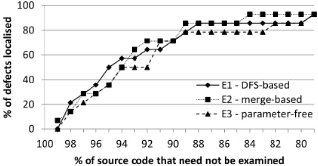
is a graphical representation of this data. Similarly to related work (e.g., [18, 20]), it represents the percentage of defects localised versus the percentage of source code that does not need to be examined.
0 20 40 60 80 100 100 98 96 94 92 90 88 86 84 82 80 % of de fe cts loc alis ed
% of source code that need not be examined
E1 ‐ DFS‐based E2 ‐ merge‐based E3 ‐ parameter‐free
Figure 4: The percentage of defects localised when not examining a certain percentage of source code.
In line with our hypothesis (see Section 4.2), the merge-based variant (E2) performs better than the pure DFS-based approach (E1) in all but four data points in Figure 4. The average values in Table 3 reflect this as well. With the merge-based variant (E2), one finds a defect by examining 6.1% of the source code on average. Not surprisingly, parameter-free defect localisation (E3) always performs worse than or equal to the parameterised variant (E2). However, it still allows a developer to find defects by inspecting 7.5% of the code on average, without having to set any parameters. Focusing on the best approach, the merge-based variant (E2), two defects are pinpointed directly, and six defects can be localised by investigating less than 10 methods. Only one defect cannot be localised at all (as before), and for only two defects 100 or more methods need to be inspected. All in all, we deem these results very helpful: On average, almost 94% of the source code can be excluded from manual debugging, and to find 86% of all defects, one can skip 89% of the code. 6 Related Work
Dynamic defect-localisation techniques analyse instru-mented programme runs, whilestatic techniques
inves-tigate the source code only. We now briefly review some work apart from call-graph mining (see Section 2).
Static Analysis. Mining software repositories maps post-release failures from a bug database to de-fects in source code. For example, [23] derives code metrics and builds regression models which then predict possible post-release failures. Such approaches rather give hints on code quality issues than pinpointing actual defects. FindBugs[2] is an approach complementary to ours. Its static code analysis for Java works well when identifying certain typical patterns of defect-prone pro-gramming, but cannot identify all sophisticated defects. Dynamic Analysis. Tarantula [18] is a coverage-analysis technique. To localise defects, it generates a ranking of statements which are executed more often in failing executions. While this technique is relatively simple, it produces good results. In the evaluation [18], it has outperformed five competing approaches. How-ever, it does not take into account how often a statement is executed within one programme run. This tends to miss certain defects such ascall-frequency affecting bugs.
AMPLE [5] analyses sequences of method calls. The
authors demonstrate that the temporal order of calls is more promising to analyse than statement coverage only. However, AMPLE only derives relatively coargrained class-level localisations. [22] also deals with se-quences, but presents afailure-detection approach. This is, it does not localise defects, but decides whether an execution is correct or not. In general, the usage of call sequences instead of statement coverage is a generali-sation which takes more structural information into ac-count. Call-graph-based techniques in turn cover more complex structural information than sequences.
SOBER [20] is a statistical defect-localisation tech-nique. It makes use of more detailed information than coverage analysis and instruments predicates on condi-tion statements and return values. It then calculates defect likelihoods: Predicates yield high values when their evaluations differ significantly in correct and fail-ing executions. SOBER has outperformed Tarantulain most situations [20]. Opposed to our approach, it does
not analyse structural properties of call graphs. Hence, detectingstructure-affecting bugs is more difficult. 7 Threads to Validity
No defect-localisation technique can localise any kind of defect – nor does ours. A direct comparison to other approaches is difficult: Many of them work on the granularity of lines instead of methods, or do not rank their results, but present unordered sets of warnings. FindBugs [2], for instance, has both of these characteristics. As many static approaches, it can identify standard defect patterns, but was not able to detect any of the more complicated real defects inRhino. One of the best dynamic approaches, Tarantula [18], generates a ranking of lines suspected to be defective. When comparing the amount of code a developer has to examine, the Tarantula evaluation only counts the actual lines listed in its ranking instead of counting all lines of all methods, as done by our approach. Another dynamic approach, SOBER[20], generates a ranking of condition predicates. This is not directly comparable to our method ranking, too.
0 20 40 60 80 100 100 90 80 70 60 50 40 30 20 10 0 % of de fe ct s loc alise d
% of source code that need not be examined
Tarantula on Space
our approach on Rhino
Tarantula on Siemens
SOBER on Siemens
Figure 5: Assessment of the results by comparing related evaluations (values taken from [18, 20]).
When looking at Tarantulaand our approach from a theoretical perspective, our approach considers more data than code coverage (but at the coarser method level). This includes (1) call frequencies, (2) subgraph contexts and (3) the information which method has called another one. This data is potentially relevant for defect localisation, e.g., to localise frequency-affecting bugs (1) and structure-affecting bugs (2, 3).
To show that our approach delivers results with about the same or even better precision as others, we compare some values in Figure 5. It contains the origi-nal data values from theTarantula[18] andSOBER[20] evaluations with the Siemens Programmes [16] and a not publicly available programme called Space ( Taran-tula only). The figure shows that our merge-based technique performs almost always better onRhinothan
Tarantula and SOBER on Siemens and a little worse
than Tarantula on Space. It is difficult to come up
with further conclusions, as the other evaluations do not deal with real defects. Furthermore, the Siemens Programmes (<1k LOC) as well as Space (≈ 6k LOC) are a lot smaller thanRhino(≈49k LOC), and it is not known how wellTarantulaandSOBERscale for this size. 8 Challenges for Data-Mining Research
The techniques developed in this study raise a number of general data-mining research questions. These ques-tions are relevant for many applicaques-tions, and we discuss them in the following:
Graph Clustering. Caused by the class hierarchy of a grown software project, class and package sizes fre-quently are very imbalanced. This leads to scalability issues. Furthermore, the manual assignment of software entities to larger units, as typically done by the software developer (e.g., of a class to a package), is often arbi-trary. To overcome such problems, it would be helpful to have natural and balanced hierarchies. This could be done by means of(weighted) graph clustering [1] on call graphs, for instance, similarly to hierarchical mining of community structures in (social) networks [15]. From a general data-mining perspective, this is interesting, be-cause our setting would provide an objective evaluation framework for graph clustering. ‘Objective’ means that clusterings of different quality are expected to yield re-sults with different localisation precision as well. This is in contrast to numerous evaluations where domain experts have decided how good the various results are.
Integrated Hierarchical Search on Graphs. Our approach processes graphs at different levels, one after the other. Although these graphs are related (by zoom-in), the analysis at the different levels is currently done separately, without benefiting from the hierarchical procedure. This is, we have not tried to identify any synergy from that relationship so far. It would be interesting to investigate how an integrated hierarchical search procedure could look like that makes use of previous results and speeds up the process. Such results might be of interest for graph mining in other application domains as well.
Weighted Subgraph Mining. In this study we analyse weighted call graphs by means of a two-step approach: frequent subgraph mining followed byfeature selection. To our knowledge, alternative approaches for an integrated analysis of weighted graphs have never been studied systematically. However, we expect that an integration would allow for much faster analyses. Furthermore, algorithms for weighted subgraph mining could be used in many domains where weighted graphs are present. The algorithms envisioned should be able to analyse tuples of numerical weights and might exploit correlations between the tuple elements.
9 Conclusions
Defect localisation is essential in software engineering. We have presented a hierarchical call-graph-based ap-proach, building on newly proposed graph representa-tions of different levels of granularity. To localise de-fects, it hierarchically analyses graphs of a coarse gran-ularity before itzooms-ininto more fine-grained graphs. This allows for the analysis of relatively large software projects. Our evaluation features defects from the field in such a project, Mozilla Rhino. The result is that the amount of source code a developer has to examine man-ually can be reduced to about 6% in our setup. To our knowledge, this is the first study applying call-graph mining to a project of this size. Besides our contribu-tions in domain-specific data mining for software en-gineering, we have identified new general data-mining research questions relevant for many domains.
Acknowledgements. We thank Valentin Dallmeier for his support foriBUGS[6] and Klaus Krogmann, Ralf H. Reussner and Andreas Zeller for fruitful discussions. References
[1] C. C. Aggarwal and H. Wang,A Survey of Clus-tering Algorithms for Graph Data, in Managing and Mining Graph Data, Springer, 2010.
[2] N. Ayewah, D. Hovemeyer, J. D. Morgenthaler, J. Penix, and W. Pugh, Using Static Analysis to Find Bugs, IEEE Softw., 25 (2008), pp. 22–29. [3] C. Chen, X. Yan, F. Zhu, J. Han, and P. S.
Yu, Graph OLAP: A Multi-Dimensional Framework for Graph Data Analysis, Knowl. Inf. Syst., 21 (2009), pp. 41–63.
[4] H. Cheng, D. Lo, Y. Zhou, X. Wang, and X. Yan, Identifying Bug Signatures Using Discrimi-native Graph Mining, in Int. Symposium on Software Testing and Analysis (ISSTA), 2009.
[5] V. Dallmeier, C. Lindig, and A. Zeller,
Lightweight Defect Localization for Java, in European Conf. on Object-Oriented Programming (ECOOP), 2005.
[6] V. Dallmeier and T. Zimmermann, iBUGS Home-page. http://www.st.cs.uni-saarland.de/ibugs/. [7] , Extraction of Bug Localization Benchmarks
from History, in Int. Conf. on Automated Software Engineering (ASE), 2007.
[8] G. Di Fatta, S. Leue, and E. Stegantova, Dis-criminative Pattern Mining in Software Fault Detec-tion, in Int. Workshop on Software Quality Assurance, 2006.
[9] F. Eichinger and K. B¨ohm, Towards Scalability of Graph-Mining Based Bug Localisation, in Int. Work-shop on Mining and Learning with Graphs, 2009. [10] , Software-Bug Localization with Graph Mining,
in Managing and Mining Graph Data, Springer, 2010.
[11] F. Eichinger, K. B¨ohm, and M. Huber, Mining Edge-Weighted Call Graphs to Localise Software Bugs, in ECML PKDD, 2008.
[12] F. Eichinger, K. Krogmann, R. Klug, and K. B¨ohm, Software-Defect Localisation by Mining Dataflow-Enabled Call Graphs, in ECML PKDD, 2010. [13] M. Hall et al., The WEKA Data Mining Soft-ware: An Update, SIGKDD Explor. Newsl., 11 (2009), pp. 10–18.
[14] J. Han and J. Gao, Research Challenges for Data Mining in Science and Engineering, in Next Genera-tion of Data Mining, Chapman & Hall/CRC, 2008. [15] J. Huang, H. Sun, J. Han, H. Deng, Y. Sun, and
Y. Liu, SHRINK: A Structural Clustering Algorithm for Detecting Hierarchical Communities in Networks, in CIKM, 2010.
[16] M. Hutchins, H. Foster, T. Goradia, and T. Os-trand,Experiments on the Effectiveness of Dataflow-and Controlflow-Based Test Adequacy Criteria, in Int. Conf. on Software Engineering (ICSE), 1994.
[17] P. M. Johnson,A Comparative Review of LOCC and CodeCount, Tech. Report CSDL-00-10, Department of Information and Computer Sciences, University of Hawaii, Honolulu, USA, 2000.
[18] J. A. Jones and M. J. Harrold, Empirical Eval-uation of the Tarantula Automatic Fault-Localization Technique, in Int. Conf. on Automated Software Engi-neering (ASE), 2005.
[19] G. Kiczales, E. Hilsdale, J. Hugunin, M. Ker-sten, J. Palm, and W. G. Griswold,An Overview of AspectJ, in European Conf. on Object-Oriented Pro-gramming (ECOOP), 2001.
[20] C. Liu, L. Fei, X. Yan, J. Han, and S. P. Midkiff,
Statistical Debugging: A Hypothesis Testing-Based Ap-proach, IEEE Trans. Software Eng., 32 (2006), pp. 831– 848.
[21] C. Liu, X. Yan, H. Yu, J. Han, and P. S. Yu, Min-ing Behavior Graphs for “Backtrace” of NoncrashMin-ing Bugs, in SDM, 2005.
[22] D. Lo, H. Cheng, J. Han, S.-C. Khoo, and C. Sun,
Classification of Software Behaviors for Failure Detec-tion: A Discriminative Pattern Mining Approach, in KDD, 2009.
[23] N. Nagappan, T. Ball, and A. Zeller, Mining Metrics to Predict Component Failures, in Int. Conf. on Software Engineering (ICSE), 2006.
[24] M. Philippsen et al., ParSeMiS Homepage.
http://www2.informatik.uni-erlangen.de/EN/ research/ParSeMiS/.
[25] J. R. Quinlan,C4.5: Programs for Machine Learning, Morgan Kaufmann, 1993.
[26] X. Yan, H. Cheng, J. Han, and P. S. Yu, Min-ing Significant Graph Patterns by Leap Search, in SIG-MOD, 2008.
[27] X. Yan and J. Han, CloseGraph: Mining Closed Frequent Graph Patterns, in KDD, 2003.
[28] A. Zeller,Why Programs Fail: A Guide to System-atic Debugging, Morgan Kaufmann, 2009.
![Figure 5: Assessment of the results by comparing related evaluations (values taken from [18, 20]).](https://thumb-us.123doks.com/thumbv2/123dok_us/1900852.2778081/11.918.108.432.527.696/figure-assessment-results-comparing-related-evaluations-values-taken.webp)