Abstract—Additive Manufacturing (AM) is becoming a field of growing interest due to its unique characteristics. Improvement in processes, materials and methods is achieving the goal of carrying AM uses from prototyping to final parts manufacturing. Polyjet process is among the most promising AM technologies, since low layer thickness and transversal resolution allows for manufacturing parts with relative dimensional and geometrical accuracy. As it becomes possible to produce parts with narrow tolerances, factors influencing measurement accuracy demand deeper analysis. This work focuses on analysing influence of sampling strategy upon accuracy when measuring dimensional and geometrical features upon Polyjet parts. Sampling size and sequence sampling have been selected as influence factors in this study, while distance between parallel planes and flatness were used as quality indicators.
Index Terms—Accuracy, Polyjet, sampling strategy
I. INTRODUCTION
TUDIES focused on improving dimensional or geometrical quality for AM parts [1]-[4] demand in-deep knowledge on how reliability of data used in their analysis gets affected by measurement conditions. 3D digitizing is used for providing a series of data that constitute a virtual representation of a surface. These data shall be later used for measurement calculations depending on the type of feature. Accuracy of these measurements should be influenced by a series of factors. Machine uncertainty, sampling strategy, part physical characteristics or ambient conditions are among the most important factors influencing measurement accuracy. In metrological laboratories, a value for each single measurement system uncertainty is completely known, whereas ambient conditions are kept under control.
Sampling strategy, on the other hand, has to be defined for each test. Different researchers have studied the influence of sampling strategy in measurement accuracy. Three categories of methods have been distinguished: “blind” methods, adaptive methods and manufacturing-based methods [5].
Blind methods distribute sampling points over the feature surface, regardless to the specific characteristics of the
Manuscript received March 14, 2014; revised Mach 28, 2014. B. J. Álvarez. is a Lecturer (e-mail: [email protected]). D. Blanco is a Full Time Lecturer (e-mail: [email protected]).
A. Noriega is a temporary Professor (e-mail: [email protected]). P. Fernández is a Lecturer (e-mail: [email protected]).
N. Beltran is an Associated Lecturer (e-mail: [email protected]) The corresponding address for all authors is: Department of Manufacturing Engineering, University of Oviedo, Campus de Gijón, 33203 Gijón, SPAIN.
inspected surface. Among this category, uniform, stratified and random methods are the most used. In the case of stratified sampling methods, Hammersley and Halton-Zaremba distributions are of particular interest due to their low discrepancy value. Discrepancy is a measure of how evenly a region is sampled with a certain distribution.
Woo and Liang [6] were the first authors that proposed low discrepancy distributions for their use in sampling strategies on CMMs. Several researchers followed their proposal and compared the results achieved with these distributions as opposed to the traditional uniform sampling that CMM software includes. Lee et al [7] showed that Hammersley sequence allows for a nearly quadratic reduction in the number of sampling points with regard to the uniform sampling when inspecting different geometries (planes, cylinders, cones and spheres). Later on, Kim and Raman [8] tested different point distributions for evaluating flatness on steel plates. Other authors dealt with the initial point location when inspecting circular features [9] assuming a uniform sampling rather than comparing different point distributions.
Adaptive methods iteratively select the most “critical” points to be measured at each step of the procedure. On the basis of an initial sampling (usually uniform), specific algorithms identify the critical areas requiring a denser sampling [10], [11]. The main drawback of adaptive sampling strategies is the amount of time required for the iterative process. Raghunandan and Rao [12] applied an adaptive technique based on the Hammersley sequence for inspecting flatness.
The third category methods are based on a previous knowledge of the geometrical errors of the part to be inspected, which is called “signature model”. Summerhays et al. [13] proposed models for form errors on internal cylindrical features. Aforementioned Rossi [11] also studied models for the roundness deviation (undulations) before applying its sampling method. Finally, Colosimo et al. [5] defined a sampling strategy by optimizing an objective function that aims at maximizing the chance of selecting points that actually affect the form error computation.
As it can be seen, sample size is a key aspect of sampling strategies. This factor has a direct relation with time and cost. A higher number of samples will cause higher digitizing times and a proportionally higher cost for the same type of sampling strategy.
Finally, part physical properties have a strong dependence on AM process characteristics [14]-[16]. Though in these studies the measured values of the characteristics are just assumed-as-true, attention should be paid to evaluate the
Influence of Sampling Strategies upon
Accuracy when Measuring PolyJet Parts
Braulio J. Álvarez, David Blanco, Álvaro Noriega, Pedro Fernández and Natalia Beltrán
possibility of part characteristics affecting repeatability or trueness. In present work, Polyjet technology has been considered for manufacturing test specimen. In this process, a layer of an acrylic-based photopolymer is jetted on a flat surface and then cured with UV radiation. The material is instantly solidified, so additional layers can be stacked one on top of the other along Z direction. According to this procedure, geometry in each layer can be precisely-constructed.
II.EXPERIMENTAL FRAMEWORK
A. Objective
The main objective of present work is to analyse the influence of sampling strategies upon measurement accuracy of Polyjet parts features.
B. Factors
Two factors have been selected in present work: the type of sampling sequence (SS) and the sample size, expressed in terms of the number of digitized points (N).
C.Quality Indicators
Two features have been selected as representative of measurement accuracy: distance between parallel planes d
and surface flatness f. For each feature, two quality parameters have been calculated in order to characterize accuracy-dependence. These parameters were the average value of a series of consecutive measurements of the same feature and the standard deviation within this series. Thus,
d represents the average value of a series of consecutively-calculated distances between parallel planes and d
represents the standard deviation of d within the same series. Similarly, f represents the average value of a series of flatness measurement of a certain surface and f represents
the standard deviation of f within the same series.
D.Materials and Methods
A Stratasys Object 30 machine has been used for manufacturing an octagonal thin-walled test specimen. Stratasys RGD240 photopolymer has been used as model material, whereas Stratasys FullCure 705 photopolymer has been used in support structures. Due to part orientation within tray, only the base of the part was supported, which allows for using only model material in the surfaces that should later be digitized. Layer thickness is 28 µm and Resolution in both X and Y directions is up to 600 dpi (approximately 42 µm).
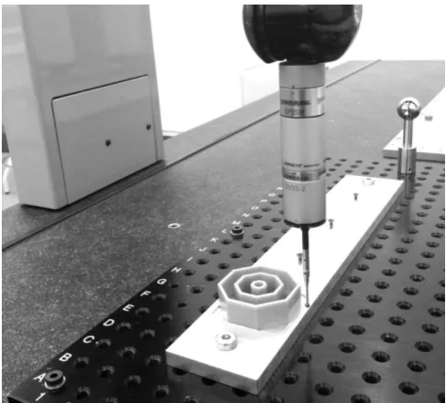
Two parallel flat surfaces with a 50 mm theoretical distance between them had been used as test features. One of these planes has been identified as the datum or reference surface and also used for flatness calculation. All measurements within this work were conducted (Figure 1) using a DEA Global Image 091508 (CMM) which Maximum Permissible Linear Error (MPEE) and Maximum
[image:2.595.304.549.48.269.2]Permissible Probing Error (MPEP) were certified as in (1).
Fig. 1. Disposition of test specimen during CMM digitizing.
3
2.3 3 10
m , being
in mm
2.2 μm
E
P
MPE
L
L
MPE
(1)III. DESIGN OF EXPERIMENTS (DOE)
Three levels corresponding each with a different point-placement strategy have been considered for the SS factor: the Hammersley sequence sampling (H), the Halton– Zaremba sequence sampling (H-Z), and the Aligned Systematic sampling (AS).
Hammersley [17] proposed a generalized sequence for n
dimensions based on the sequence of van de Corput [18]. In Hammersley sequence, the coordinate of the first dimension depends on the sampling size. For the rest of dimensions, the coordinate is obtained from the inverse radical function taking the first prime numbers as bases. For the bidimensional case, taking the prime number 2 as the basis, the Hammersley sequence is reflected in (2):
1 1
0 2
i
k j
i ij
j
i x
N
y b
(2)
where N is the total number of sample points; i [0, N – 1];
bi is the binary representation of the index i, bij is the jth bit
in bi; and k is log2N.
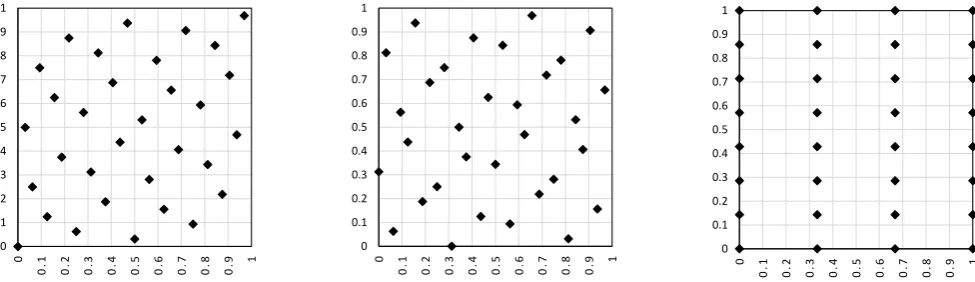
0 0.1 0.2 0.3 0.4 0.5 0.6 0.7 0.8 0.9 1 0 0 .1 0 .2 0 .3 0 .4 0 .5 0 .6 0 .7 0 .8 0 .9 1 0 0.1 0.2 0.3 0.4 0.5 0.6 0.7 0.8 0.9 1 0 0 .1 0 .2 0 .3 0 .4 0 .5 0 .6 0 .7 0 .8 0 .9 1 0 0.1 0.2 0.3 0.4 0.5 0.6 0.7 0.8 0.9 1 0 0 .1 0 .2 0 .3 0 .4 0 .5 0 .6 0 .7 0 .8 0 .9 1
Fig. 3. Distribution of 32 points (N) for different sampling sequences: Hammersley (left), Halton-Zaremba (center) and Aligned Systematic (right).
1 ( ) 0 1 ' 1 0 ' ' 2 2
1 for odd
otherwise k k j i ij j k j i ij j ij ij ij ij i x b N y b
b b j
b b
(3)However, to use this method, there is a restriction on the sample points that the number be a power of 2.
Finally, the aligned systematic sampling is a uniform sampling method. In the bi-dimensional case of a flat surface, a grid defined by a rows and b columns is established and a point is located in each vertex of the grid. For sampling N points, the method for defining the grid is as follows; first, the integer divisors of N are found, second, the two divisors with less difference between them whose product would be equal to N are selected as a and b, and lastly, the point coordinates are established at each vertex of the grid. For example, the coordinates of a point located at the vertex where the i row intersects the j column are (4):
1 1 i x a j y b (4)
Note that this method distributes points in the boundary vertices of the flat region, whereas the first two methods only place a single point at the region boundary.
In a similar way, five levels have been considered for N:
4, 8, 16, 32 and 64 points. These levels have been selected because they represent typical sampling 2m sizes used in testing, while also allow for comparing alternate sampling sequences.
A full-factorial DOE has been defined considering 3x5 experiments. Figure 3 contains a representation of sampling distribution corresponding to all the sampling sequences considered in this work and particularized for level 32 of factor N. For each single combination of levels both test surfaces have been digitized fifteen times consecutively under repeatability conditions (in a short period of time) digitized and resultant d , d f , and f have been
thereafter calculated. This procedure has been replicated two
times, so that a total number of 30 experimental runs have been performed. Due to the time required for each experimental run (approximately four hours), both replicates have been blocked, as repeatability conditions cannot be assured for different blocks.
IV. RESULTS
A. Behaviour of Distance between Parallel Planes
Both SS and N factors apparently have an influence upon average distance between parallel planes. According to Figure 4, mean values for d are maximum for the HZ
distribution and minimum for the AS distribution.
H-Z H AS 50.0877 50.0876 50.0875 50.0874 50.0873 50.0872 50.0871 50.0870 64 32 16 8 4 Sampling M e a n ( m m ) Points Main Effects Plot for Average
[image:3.595.308.544.390.551.2]Data Means
Fig.4. Main effects plots ford.
The maximum sample size (64) provides a higher value than the rest of sizes, but its behaviour has not a clearly-defined tendency, with sharp slope changes between levels. Nevertheless, these results cannot be properly analysed without considering interaction effects between factors (Figure 5).
Thus, mean values present a 2 µm variation within experimental range. The number of samples shows neatly different influence for different sample distributions. Therefore, a higher sample size causes an increase on distance estimation for the AS sample strategy, whereas opposite effect (a reduction of distance values) is clearly present in H sample distribution. H-Z, on the other side, does not present a clearly-defined behaviour, as a W-shaped profile reflects huge variation of mean distribution.
Combined effects of AS, H and H-Z behaviour with N
64 32 16 8 4 50.0885
50.0880
50.0875
50.0870
50.0865
Points
M
e
a
n
(
m
m
)
AS H H-Z Sampling Interaction Plot for Average
[image:4.595.308.548.193.346.2]Data Means
Fig. 5. Interaction plots for d
The ANOVA reflected in Table I provides further information on this indicator. As it can be seen through p-values, variance of d cannot be properly explained considering SS, whereas N and the combination of SS and N
have a significant influence.
The ANOVA also reveals that differences between blocks are really significant. This implies that the amount of variance that can be related to differences in measuring conditions (mainly slight temperature variations) have greater influence upon measurement results than the rest of considered factors.
TABLEI
ANALYSIS OF VARIANCE FOR d
Source DF Seq SS Adj SS Adj MS F P Block 1 0.0000423 0.0000423 0.0000423 375.66 0.000 SS 2 0.0000006 0.0000006 0.0000003 2.64 0.107 N 4 0.0000016 0.0000016 0.0000004 3.52 0.035 SS*N 8 0.0000126 0.0000126 0.0000016 14.03 0.000 Error 14 0.0000016 0.0000016 0.0000001 375.66 0.000 Total 29 0.0000587
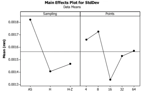
Effect of factors influencing repeatability of measures expressed in terms of standard deviation through the dcan
be observed in Figure 6. H and H-Z distributions provide comparatively lower values for the standard deviation, while the effect of sample size cannot be so clearly understand without considering interaction effects, even when minimum values are reached for 16 samples.
H-Z H
AS 0.0018
0.0017
0.0016
0.0015
0.0014
0.0013
64 32 16 8 4 Sampling
M
e
a
n
(
m
m
)
Points Main Effects Plot for StdDev
Data Means
Fig. 6. Main effects plots ford
Interaction plot (Figure 7) allows for clarifying cross-dependence between these two factors. Thus, d gets worse
with an increased sample size for AS sampling, whereas this effect is clearly opposite for the H and H-Z sampling strategies. Minimum d values for the 16 samples can be
explained by a simultaneous combination of relatively-low values within the three strategies contemplated in this work.
Nevertheless, the interaction plot reveals that H and H-Z
strategies tend to minimize d when a sampling size equal
or above 16 samples has been used.
64 32 16 8 4 0.0025
0.0020
0.0015
0.0010
Points
M
e
a
n
(
m
m
)
AS H H-Z Sampling Interaction Plot for StdDev
[image:4.595.46.291.396.508.2]Data Means
Fig. 7. Interaction plots ford
Results from the ANOVA (Table II) indicate that all factors considered have an influence on variance results. Second-order interaction is also important, so that selection of optimal or recommended values for sampling strategies has to simultaneously consider both distribution and number of samples.
TABLEII ANALYSIS OF VARIANCE FOR d
Source DF Seq SS Adj SS Adj MS F P Block 1 0.0000025 0.0000025 0.0000025 178.50 0.000 SS 2 0.0000010 0.0000010 0.0000005 36.22 0.000 N 4 0.0000005 0.0000005 0.0000001 9.40 0.001 SS*N 8 0.0000091 0.0000091 0.0000011 81.60 0.000 Error 14 0.0000002 0.0000002 0.0000000 178.50 0.000 Total 29 0.0000132
B. Behaviour of Flatness
According to Figure 8, mean values for f have are strongly dependant on N, whereas SS has a reduced influence.
[image:4.595.304.551.474.582.2] [image:4.595.51.287.618.771.2]H-Z H
AS 0.016 0.014 0.012 0.010 0.008 0.006 0.004 0.002
64 32 16 8 4 Sampling
M
e
a
n
(
m
m
)
Points Main Effects Plot for Average
[image:5.595.52.288.54.223.2]Data Means
Fig. 8. Main effects plot for f .
These results clarify main effects for sampling behaviour as it can be observed how flatness is clearly underrated when 4 or 8 sample sizes are employed. From these results, it should be stated that a minimum 16 samples size should be used if flatness has to be calculated from digitized data.
64 32 16 8 4 0.025
0.020
0.015
0.010
0.005
0.000
Points
M
e
a
n
(
m
m
)
AS H H-Z Sampling Interaction Plot for Average
[image:5.595.305.544.309.467.2]Data Means
Fig. 9. Main effects plot for f .
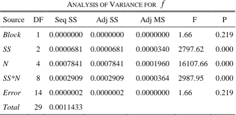
ANOVA results (Table III) do confirm N relevance, but also indicate that SS has a significant influence on flatness values. Interaction is also significant. On the other side, according to p-value, blocked data have not a significant influence on flatness measured values. This circumstance is consistent with the effect observed for distance quality indicator: whereas d should be influenced by dimensional drift related to slight variations on temperature, these variations should not have an equivalent influence upon flatness.
TABLEIII
ANALYSIS OF VARIANCE FOR f
Source DF Seq SS Adj SS Adj MS F P
Block 1 0.0000000 0.0000000 0.0000000 1.66 0.219 SS 2 0.0000681 0.0000681 0.0000340 2797.62 0.000 N 4 0.0007841 0.0007841 0.0001960 16107.66 0.000 SS*N 8 0.0002909 0.0002909 0.0000364 2987.95 0.000 Error 14 0.0000002 0.0000002 0.0000000 1.66 0.219 Total 29 0.0011433
TABLEIV ANALYSIS OF VARIANCE FOR f
Source DF Seq SS Adj SS Adj MS F P Block 1 0.0000000 0.0000000 0.0000000 0.06 0.805 SS 2 0.0000000 0.0000000 0.0000000 0.28 0.759 N 4 0.0000001 0.0000001 0.0000000 4.40 0.016 SS*N 8 0.0000001 0.0000001 0.0000000 3.85 0.014 Error 14 0.0000001 0.0000001 0.0000000 0.06 0.805 Total 29 0.0000000
Finally, correspondent ANOVA (Table IV) does reveal that variance f is not significantly affected by SS and,
moreover, blocked results does not show any influence on these parameter values (Table).
Main effects (Figure 10) and Interaction (Figure 11) indicate that selection of SS does only have an influence upon results when it is considered alongside with sampling size N.
H-Z H AS 0.00022 0.00020 0.00018 0.00016 0.00014 0.00012 0.00010 0.00008 0.00006
64 32 16 8 4 Sampling
M
e
a
n
(
m
m
)
Points Main Effects Plot for StdDev
[image:5.595.51.288.310.469.2]Data Means
Fig. 10. Main effects plot for f .
According to these results, a minimum 16 points should be recommended, whereas considering H or H-Z distribution will cause differences lower that 0.1 µm when doubling from 16 to 32 samples.
64 32 16 8 4 0.00040 0.00035 0.00030 0.00025 0.00020 0.00015 0.00010 0.00005
Points
M
e
a
n
(
m
m
)
AS H H-Z Sampling Interaction Plot for StdDev
Data Means
Fig. 11. Interaction plot for f.
V.CONCLUSIONS
[image:5.595.47.291.637.756.2]Slight differences in ambient temperature, even in laboratory-controlled conditions (20 ± 0.2 ºC during the experimental runs), could have a significant influence when distances between planes are measured. Standard deviation of distance measurements are also affected by this effect. On the other hand, no dependence of flatness measurements with variability of measurements conditions has been found. Since no values for the thermal expansion coefficient are available for this material, further investigations should take care of this lack of information. The dependence of thermal expansion coefficient with layer orientation is another factor that should be considered.
As a general result, a minimum 16 samples with a Hammersley distribution should be recommended for properly digitizing Polyjet surfaces. Within the limits of this experimentation, using 16 samples will lead to approximately 1 µm standard deviation for distance measurements, which is low enough as compared with the 42 µm XY resolution of the Object 30 Polyjet machine. Equally, standard deviation for flatness measurements should be below 0.12 µm.
Additionally, results indicate that a sample size above 16 samples will be also adequate when using Halton-Zaremba distribution, whereas Aligned Systematic provides worse results for all the analysed parameters.
Finally, whereas repeatability values are among system capacity, notable variations in averaged parameters have to be considered when an optimization analysis is conducted upon Polyjet parts. Material temperature-dependence could be affecting interpretation of results, especially when measures have been conducted in different time periods.
REFERENCES
[1] D. Y. Chang and B. H. Huang, “Studies on profile error and extruding aperture for the RP parts using the fused deposition modeling process,” The International Journal of Advanced Manufacturing Technology, vol. 53, no. 9–12, pp. 1027–1037, Apr. 2011.
[2] I. El-Katatny, S. H. Masood and Y. S. Morsi, “Error analysis of FDM fabricated medical replicas,” Rapid Prototyping Journal, vol. 16, no. 1, pp. 36–43, 2010.
[3] A. K. Sood, R. K. Ohdar and S. S. Mahapatra, “Improving dimensional accuracy of Fused Deposition Modeling processed part using grey Taguchi method,” Materials & Design, vol. 30, no. 10, pp. 4243–4252, Dec. 2009.
[4] A. Noriega, D. Blanco, B. J. Alvarez and A. Garcia, “Dimensional accuracy improvement of FDM square cross-section parts using artificial neural networks and an optimization algorithm,” The International Journal of Advanced Manufacturing Technology, vol. 69, no. 9–12, pp. 2301–2313, Dec. 2013.
[5] B. M. Colosimo, G. Moroni and S. Petrò, “A tolerance interval based criterion for optimizing discrete point sampling strategies,” Precision Engineering, vol. 34, no. 4, pp. 745–754, Oct. 2010.
[6] T. C. Woo and R. Liang, “Dimensional measurement of surfaces and their sampling,” Computer-Aided Design, vol. 25, no. 4, pp. 233– 239, Apr. 1993.
[7] G. Lee, J. Mou and Y. Shen, “Sampling strategy design for dimensional measurement of geometric features using coordinate measuring machine,” International Journal of Machine Tools and Manufacture, vol. 37, no. 7, pp. 917–934, Jul. 1997.
[8] W.-S. Kim and S. Raman, “On the selection of flatness measurement points in coordinate measuring machine inspection,” International Journal of Machine Tools and Manufacture, vol. 40, no. 3, pp. 427– 443, Feb. 2000.
[9] F. M. M. Chan, T. G. King and K. J. Stout, “The influence of sampling strategy on a circular feature in coordinate measurements,” Measurement, vol. 19, no. 2, pp. 73–81, Oct. 1996.
[10] R. Edgeworth and R. G. Wilhelm, “Adaptive sampling for coordinate metrology,” Precision Engineering, vol. 23, no. 3, pp. 144–154, Jul. 1999.
[11] A. Rossi, “A form of deviation-based method for coordinate measuring machine sampling optimization in an assessment of roundness,” Proceedings of the Institution of Mechanical Engineers, Part B: Journal of Engineering Manufacture, vol. 215, no. 11, pp. 1505–1518, Nov. 2001.
[12] R. Raghunandan and P. Venkateswara Rao, “Selection of an optimum sample size for flatness error estimation while using coordinate measuring machine,” International Journal of Machine Tools and Manufacture, vol. 47, no. 4-5, pp. 477–482, Mar. 2007. [13] K. D. Summerhays, R. P. Henke, J. M. Baldwin, R. M. Cassou and C.
W. Brown, “Optimizing discrete point sample patterns and measurement data analysis on internal cylindrical surfaces with systematic form,” Precision Engineering, vol. 26, no. 1, pp. 105– 121, Jan. 2002.
[14] A Bellini and S. Güçeri, “Mechanical characterization of parts fabricated using fused deposition modelling,” Rapid Prototyping Journal, vol. 9, no. 4, pp. 252–264, 2003.
[15] S. H. Ahm, M. Montero, D. Odell, S. Roundy and P.K. Wright, “Anisotropic material properties of fused deposition modeling ABS,” Rapid Prototyping Journal, vol. 8, no. 4, pp. 248–257, 2002. [16] A. Pilipović, P. Raos and M. Šercer, “Experimental analysis of
properties of materials for rapid prototyping,” The International Journal of Advanced Manufacturing Technology, vol. 40, no. 1–2, pp. 105–115, Jan. 2009.
[17] J. Hammersley, “Monte Carlo methods for solving multivariable problems,” Proceedings of the New York Academy of Science, 86, pp. 844–874, 1960.
[18] J. G. van der Corput, “Verteilungsfunktionen. I, II,” Proceedings of the Koninklijke Nederlandse Academie van Wetenschappen. Series B: Physical Sciences, 38, pp. 813–821 and 1058–1066, 1935. [19] J. Halton, “On the efficiency of certain quasi-random sequences of
points in evaluating multi dimensional integrals,” Numerische Mathematik, 2, pp. 84-90, 1960.