Classification of Brain Tumor Grades using Neural
Network
B.Sudha, P.Gopikannan, A.Shenbagarajan, C.Balasubramanian
Abstract- In this paper, the automated classification of brain tumor grades using FFNN, MLP and BPN are performed. The features of the brain tumor grades are extracted using GLCM and GLRM. The optimal features are selected using fuzzy entropy measure. Based on the features that are extracted from the various grades of brain tumor MRIs, the classifiers are trained and tested. The performances of the classifiers are evaluated in both the testing and training phases with various parameters. These classifiers are tested using a dataset of 50 MR brain images. From the accuracy in classifying the tumor grades, it is found that BPN outperforms other classifiers with the classification accuracy of 96.7% and this will be the fruitful automated tool for the classification of brain tumors according to their grades.
Keywords- Classifier, Feature Extraction, Feature Selection, Neural Network, Statistical Features
I. INTRODUCTION
Now-a-days the major reason for death among the people is brain tumors. The automated system to identify brain tumors will help the patients in their early diagnosis. Depending on the grades of the tumor, treatment will vary. Hence the automatic classification of brain tumor grades by the system from the brain MRI is essentially a need for the patients for their survival. The proposed system is designed in order to classify the type of tumor based on its features that are extracted from the segmented tumor region of brain image.
Deepa and Aruna Devi (2012) compared the performance of BPN and RBFN classifier for the classification of MR brain images. They simply found whether the brain image is normal or abnormal and they have not found out its grades if it is tumorous. They concluded that RBFN classifier is best suited for the classification of brain tumors.
Manuscript received 7 April ,2014.
B.Sudha is the PG Scholar in PSR Rengasamy College of Engineering for
Women, Sivakasi, Tamilnadu, India (email:sudhabalasubramanian.mepco@gmail.com)
P.Gopikannan is the Assistant Professor in PSR Rengasamy College of Engineering for women, Tamilnadu, India (email: gopikannan@psrr.edu.in) A.Shenbagarajan is the Assistant Professor in PSR Rengasamy College of Engineering for women, Sivakasi, India (email: shenbagarajan@psrr.edu.in)
C.Balasubramanian is the Professor in PSR Rengasamy College of Engineering for women,Sivakasi, Tamilnadu, India (email: bala@psrr.edu.in)
Sandeep et al. (2006) developed the neural network and support vector machine classifiers for the classification of brain images. Features extracted using wavelets are fed as inputs to the neural network classifier. Discrete Wavelet Transform uses the discrete set of wavelets to implement the wavelet transform[15]. SVM is the binary classification method that takes input from two classes and produces the output as the model file for the classification of data into the corresponding classes. Neural network is the non-linear computational unit through which large class of patterns can be recognized. The performances of both these classifiers are evaluated and based on this neural network is found to be the efficient classifier.
Arthi et al.(2009) [1], proposed the hybrid of neural network and fuzzy technique for the diagnosis of hyperactive disorder. A combination of self organizing maps which is unsupervised technique and radial basis function which is supervised algorithm. In Self Organizing Map, learning process is carried out and learning parameter rate starts to decrease during the convergence phase. Radial Basis Function neural network is a supervised technique for the non-linear data and in this no hidden layer units are present. Based on the degree of sensitivity to inputs, the hidden units in neural network are assigned with equal weights. They concluded that hybridization of these methods involves complexity and relaxation of training dataset is not possible in such scenarios.
Mohanaiah et al (2013) extracted the texture features such as energy, homogeneity, correlation, entropy using the GLCM. They have extracted the texture features for the images of varying sizes 64×64, 128×128, 256×256. They concluded that when the image size increases, the feature values are also increasing. Hence the optimum size of 128×128 is best suited for feature extraction and this will result in minimum loss of information.
Dong-Hui Xu et al proposed the run length metric for the extraction of features from images. The run length matrix is used to extract the features from 3D liver image. The features such as SRE, LRE, LGRE, SGRE and many others are extracted. They found out the features from CT liver image which is in 3D form. The run length matrices are calculated in various directions. They concluded that the results obtained from 2D data and those obtained from volumetric data have some similarities as well as differences.
II. PROPOSED SYSTEM
The proposed system for the classification of brain tumors can be done by first extracting its features and the flow diagram is shown in fig1.
[image:2.595.49.286.134.459.2]
Fig 1: Flow diagram for the proposed system
A. Feature Extraction
The content of the image can be described by its features. The need for feature extraction is that the relevant information is extracted from the tumor region in order to perform the classification of tumor grades. Various features such as color, shape and texture are used to represent the input. Features can be of two types: general features and domain specific features. General features include pixel level features, local and global features. Application specific features vary depending on the type of application for which the feature is to be extracted. Color information is represented using the color models and based on the similarity of color models. Color feature is used as the visual features in image retrieval.
Texture is one of the features to describe the characteristic of image. Texture is defined as the repeating pattern that occurs frequently in the image. Shape based image retrieval is based on measuring the similarity between shapes which denotes the features. Statistical texture features specifies the statistical distribution of intensity at the specified points relative to each other in the image. Statistical features can be classified into first-order, second-order and higher-order statistics.
1) GLCM Based Feature Extraction:
Gray Level Coocurrence Matrix(GLCM) is used to extract second-order statistical features. GLCM is a matrix which can be formed by considering the number of gray levels which is equal to the number of rows and columns of the matrix. The number of gray levels in the image determines the size of glcm. The relative frequency P(i,j|Δx,Δy) between two pixels having intensities i and j and let the distance between two pixels be (Δx,Δy) and this forms the matrix element. The performance of the GLCM based feature depends on the number of gray levels used.
Correlation is the measure of linear dependency of pixels at locations that are relative to one another. It is given as
,
1 1
0 0
i j P i j
G G x y
Correlation
x y
i j
(1.1)
where xand y are the mean values obtained from P x and P y.
xand y are the standard deviation values of
P x and P y.
G is the number of gray levels.
Entropy measures the information present in the image. Homogeneous pixels of the image have high entropy. Entropy is given as
1 1
, log ,
0 0
G G
Entropy P i j P i j
i j
(1.2)
Inverse Difference Moment is the measure of local homogeneity. It is low for inhomogeneous images.
1 1 1
, 2 0 0 1
G G
IDM P i j
i j i j
(1.3)
Energy is the measure of image homogeneity. It is the sum of squares of entries in the GLCM. Energy can be defined as
1 1 2
0 0
G G
Energy Pij
i j
(1.4)
Contrast can be measured by the local intensity variation of the image and it is given by,
1 2 ,
0 1 1
G G G
Contrast n P i j
n i j
(1.5)
2) Gray Level Run Length Matrix:
Run is defined as the consecutive pixels that have the same gray level intensity along specific orientation. Fine textures contain short run with similar gray level intensities whereas coarse textures contain long run with different intensities.
The elements in the run length matrix P(i,j) is defined in which the number of runs with pixels of gray level intensity equal to i and length of run equals to j which is the specific orientation.
Feature Selection using Fuzzy Entropy Measure GLCM Feature
Extraction
GLRM Feature Extraction
Database
Training Phase Testing Phase
Classification
FFNN MLPN
BPNN Segmented tumor region
Short Run Emphasis is the measure of short runs which are distributed and it is meant for fine textures. Short Run Emphasis is given as
1 ( , ) 2 1 1 M N P i j SRE
nri j j
(1.6)
Long Run Emphasis is the measure of long runs and it is mainly for coarse textures. It is defined as
1 2
, 1 1M N
LRE j P i j
nr i j
(1.7)
Low GrayLevel Run Emphasis is the measure of distribution of low gray level values and it is given as
1 ( , )2 1 1 M N P i j LRGE
nri j i
(1.8)
High GrayLevel Run Emphasis is the measure of distribution of high gray level values and denoted as
1
, 21 1 M N
HRGE P i j i
nr i j
(1.9)
B. Feature Selection
Feature selection is the process to select the important features by removing the redundant and insignificant features. The need for feature selection is that it will increase the classifier accuracy. Feature selection is carried out using fuzzy entropy measure. Fuzzy entropy denotes the fuzziness of a fuzzy set. Degree to which the data is ambiguous denotes the fuzziness of the fuzzy set and membership is assigned to the data by which the entropy is obtained.
Generally entropy is the measure of randomness. The amount of uncertainty from the outcome of random experiment gives the entropy measure. The feature selection task can be formulated as follows: given a feature set Y = (y1; y2; :::; yn) and a subset Z = (y1; y2; :::; yk) of Y with k
< n, which optimizes an objective function W(Y).
The fuzzy entropy measures will be used in feature selection process to evaluate the relevance of different features in the feature set, this is done by discarding those features with highest fuzzy entropy value in our training set: if the entropy value is high we assume that the feature is not contributing much for the deviation between classes, then it will be removed in our feature set. This process will be repeated for all features in the training set. The higher the similarity values are, the lower the entropy values are.
C. Classification
Classification is the process to assign a new data to the predefined data set. It is one of the major decision making process of human activity. Classification of tumors is the case in which the system can correctly predict the tumor grade with a rare shape which is distinct from all members of the training set. An artificial network consists of a pool of simple processing units which communicate by sending signals to each other over a large number of weighted connections. Each unit performs a relatively simple job receive input from neighbours or external sources and use
this to compute an output signal which is propagated to other units. Apart from this processing a second task is the adjustment of the weights. The system is inherently parallel in the sense that many units can carry out their computations at the same time.
1) Feed Forward Neural Network:
Feedforward networks have one-way connections from input to output layers. They are most commonly used for prediction, pattern recognition, and nonlinear function fitting. Supported feedforward networks include feedforward backpropagation, cascade-forward backpropagation, feedforward input-delay backpropagation, linear, and perceptron networks.
Feedforward networks, where the data flow from input to output units is strictly feed forward. The data processing can extend over multiple layers of units but no feedback connections are present that is connections extending from outputs of units to inputs of units in the same layer or previous layers. Here the inputs perform no computation and hence their layer is not counted.
A two-layer feed-forward network, with sigmoid hidden and output neurons can classify vectors arbitrarily well, given enough neurons in its hidden layer. The network will be trained with scaled conjugate gradient backpropagation. Training automatically stops when generalization stops improving, as indicated by an increase in the mean square error of the validation samples.
2) MLP:
Multilayer perceptron is a multilayer feedforward network. A MLP consists of an input layer, several hidden layers, and an output layer. It includes a summer and a nonlinear activation function. Feedforward networks often have one or more hidden layers of sigmoid neurons followed by an output layer of linear neurons. Multiple layers of neurons with nonlinear transfer functions allow the network to learn nonlinear and linear relationships between input and output vectors. The linear output layer lets the network produce values outside the range -1 to +1. Network architecture is determined by the number of hidden layers and by the number of neurons in each hidden layer. The network is trained by the backpropagation learning rule. The correct classification function is introduced as the ratio of number of correctly classified inputs to the whole number of inputs. With each combination of numbers of neurons in the hidden layers the multilayer perceptron is trained on the train set, the value of correct classification function for the train set is stored.
3) BPNN:
training set. The training of the network was performed under back propagation of the error. The trained networks were then be used to predict labels of the new data.
During the first stage’ which is the initialization of weights, some small random values are assigned. During feed forward stage each output unit (Xi) receives an input signal and transmits this signal to each of the hidden units z1, z2...zp. Each hidden unit then calculates the activation function and sends its signal to each output unit. The output unit calculates the activation function to form the response of the net for the given input pattern. During back propagation of errors, each output unit compares its activation yk with its target value tk to determine the
associated error for that pattern with that unit. Based on the error, factor δk (k=1, ...m) is computed and is used to
distribute the error at output unit back to all units in the previous layer. Similarly δj (j=1,...p) is computed for each
hidden unit zj. During final stage, the weights and biases are
updated using the δ factor and the activation.
III. EXPERIMENTAL RESULTS AND ANALYSIS
The image datasets were implemented (Matlab 2009a) for BPN, FFNN and MLPN, tested and compared. Each algorithm was trained and tested for each dataset, under the same model (kernel with the corresponding parameters) in order to achieve the same accuracy. The feed forward BPN for neural framed by generalizing the Widrow-Hoff learning rule to multiple layer network and non- linear differentiable transfer function is implemented with learning rate 0.5 and momentum factor as 0.95. Activation function maps the output of the summing junction into the final output. A value of less than 0.5 is labeled as 0 and the network classify the input image features as benign images. A value of more than 0.5 is labeled as 1 and the neural network classify the input image features as malign images. The accuracies of all classifiers, achieved for each specific dataset, were calculated under the same validation scheme, i.e., the same validation method and the same data realizations.
[image:4.595.311.544.59.168.2]In order to evaluate the classification efficiency, two metrics have been computed: (a) the training performance (i.e. the proportion of cases which are correctly classified in the training process) and (b) the testing performance (i.e. the proportion of cases which are correctly classified in the testing process). Basically, the testing performance provides the final check of the NN classification efficiency, and thus is interpreted as the diagnosis accuracy using the neural networks support.
Table I: Features extracted using GLCM
Images Contrast Correlation Homogeneity Energy Entropy Brainim1 0.1181 0.9195 0.9978 0.9680 0.2367 Brainim2 0.1068 0.9167 0.9781 0.9512 0.2895 Brainim3 0.1174 0.9098 0.9812 0.9487 0.2510 Brainim4 0.1190 0.9201 0.9645 0.9432 0.2712 Brainim5 0.1126 0.8978 0.9928 0.9716 0.3864 Brainim6 0.1082 0.8955 0.9651 0.9827 0.2619 Brainim7 0.1149 0.9189 0.9806 0.9715 0.2761
Table II: Features extracted using GLRLM
Images SRE LRE LGRE HGRE Brainim1 0.2922 19617.4063 0.4504 139.2063 Brainim2 0.2863 19305.4300 0.3968 146.0817 Brainim3 0.3112 19800.1732 0.4218 134.8400 Brainim4 0.2765 19512.8090 0.4700 131.7809 Brainim5 0.3076 19024.9126 0.4197 149.2504 Brainim6 0.3391 19638.6307 0.4938 137.7429 Brainim7 0.2500 19520.8053 0.3880 135.7402
TableI shows the features of the MR brain images extracted using GLCM and this is the sample dataset. GLRLM features extracted for the same data set is shown in TableII.
From all these features, only the relevant features are selected using the fuzzy entropy measure. Based on those features only the classifier is trained.
The performance of the classifier can be estimated using the following equations:
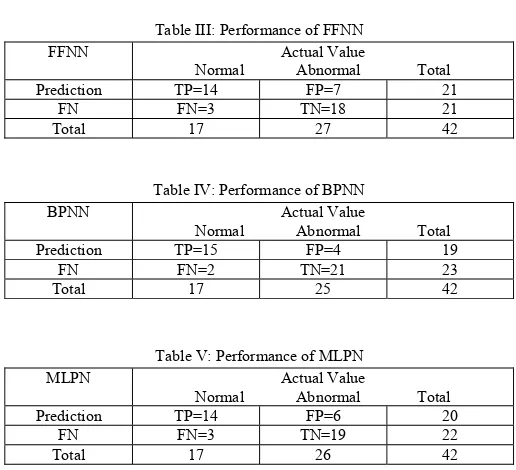
[image:4.595.297.555.328.563.2]Sensitivity (true positive fraction) = TP/TP+FN (3.1) Specificity (true negative fraction) = TN/TN+FP (3.2) Accuracy = TP+TN/TP+TN+FP+FN (3.3)
Table III: Performance of FFNN
FFNN Actual Value
Normal Abnormal Total
Prediction TP=14 FP=7 21
FN FN=3 TN=18 21
Total 17 27 42
Table IV: Performance of BPNN
BPNN Actual Value
Normal Abnormal Total
Prediction TP=15 FP=4 19
FN FN=2 TN=21 23
Total 17 25 42
Table V: Performance of MLPN
MLPN Actual Value
Normal Abnormal Total
Prediction TP=14 FP=6 20
FN FN=3 TN=19 22
Total 17 26 42
[image:4.595.299.557.641.685.2]The input data involved 42 patients (25 abnormal and 17 normal).The numbers of normal images for training set is 30 whereas for abnormal images are 12.
Table VI: Comparison of classifiers
Indices FFNN MLPN BPN Accuracy 76.19% 85.09% 96.7%
Sensitivity 82.3% 76% 72%
Specificity 88.23% 86.75% 84%
[image:4.595.40.290.656.767.2]Fig 2: ROC for FFNN
Fig 3: ROC for MLPN
Fig 4: ROC for BPNN
IV. CONCLUSION
The automated classification of brain tumor grades using various neural network classifiers is discussed. The performance of these classifiers on the collected data set is measured using sensitivity, specificity and accuracy. The accuracy of the classifier mainly depends on the optimal features based on which it is trained.
The problem is in selecting the optimal features to distinguish between the classes. More optimization requires the selection of best feature subset. Algorithm extensions can be done by incorporating the spatial autocorrelation by
fusion at different levels which reduces the mean square error in each case.
Further research issues can be improved using kernel caching techniques and moment features can also be extracted to classify the different grades of the tumor. It appears that ANN could be a valuable method to statistical methods.
REFERENCES
[1] K. Arthi & A. Tamilarasi, “Hybrid model in prediction of adhd using artificial neural networks”, International Journal of Information Technology and Knowledge Management , June 2009,vol. 2, no. 1, pp. 209-215
[2] E.A. El-Dahshan, T. Hosny, A. B. M.Salem,“Hybrid intelligent techniques for MRI brain images classification”, Digital Signal Processing, vol.20,issue 2, pp. 433-441, 2010.
[3] Qurat-ul-ain ,Ghazanfar Latif, Sidra Batool Kazmi, M.Arfan Jaffar, Anwar M.Mirza, “Classification and Segmentation of Brain Tumor using Texture Analysis”, International Conference on Recent advances in artificial Intelligence,Knowledge Engineering and Databases, pp:147-155, 2010.
[4] Lee H., Cho S., Shin M. Supporting Diagnosis of Attentiondeficit Hyperactive Disorder with Novelty Detection.
Artificial Intelligence in Medicine, 42, (3), 199–212,2008.
[5] M Wang, M. J. Wu, J. H. Chen, C. Y Yu, “Extension Neural Network Approach to Classification of Brain MRI”, 2009 Fifth International Conference on Intelligent Information Hiding and Multimedia Signal Processing, pp: 515-517, 2009.
[6] M. Varma and B. R. Babu. More generality in efficient multiple kernel learning”,In Proceedings of the International Conference on Machine learning ,Canada ,pp:1065-1072, 2009.
[7] Qurat-ul-ain ,Ghazanfar Latif, Sidra Batool Kazmi, M.Arfan Jaffar,Anwar M.Mirza, “Classification and Segmentation of
Brain Tumor using Texture Analysis”, International Conference on Recent advances in artificial Intelligence,Knowledge Engineering and Databases, pp:147-155, 2010.
[8] Ibrahiem M, Ramakrishnan S., “On the application of various probabilistic neural networks in solving different pattern classification problems”, World Applied Sciences Journal,vol.4,pp:772-780,2008.
[9] Kai Xiao, Sooi Hock Ho, Aboul Ella Hassanien, “Brain magnetic resonance image lateral ventricles deformation analysis and tumour prediction”, Malaysian Journal of Computer Science, vol. 20, no.2,pp:115-132 , 2007
[10] S.N.Sivanandam,S.Sumathi,S.N.Deepa, “Introduction to neural networks using Matlab 6”,Tata Mc Graw Hill P Ltd, 2009. [11] M. Varma and B. R. Babu. More generality in efficient multiple
kernel learning”,In Proceedings of the International Conference onMachine learning ,Canada ,pp:1065-1072, 2009.
[12] C. M Wang, M. J. Wu, J. H. Chen, C. Y Yu, “Extension Neural Network Approach to Classification of Brain MRI”, 2009 Fifth International Conference on Intelligent Information Hiding and Multimedia Signal Processing, pp: 515-517, 2009.
[13] Mammadagha Mammadov ,Engin tas ,”An improved version of backpropagation algorithm with effective dynamic learning rate and momentum “ ,Inter.Conference on Applied Mathematics
,pp:356-361, 2006.
[14] Messen W, Wehrens R, Buydens L, “Supervised Kohonen networks for classification problems“,Chemometrics and Intelligent Laboratory Systems, vol.83,pp:99-113,2006.
[15] Sandeep Chaplot, Patnaika L.M, Jagannathan N.R, “Classification of magnetic resonance brain images using wavelets as input to support vector machine and neural network”, Biomedical Signal Processing, Elsevier, Vol 1,pages
86-92,2006
0
0.2 0.4 0.6 0.8 1
0 0.2 0.4 0.6 0.8 1
False Positive Rate
True Positive Rate
ROC Curve
FFNN
0 0.2 0.4 0.6 0.8 1
0 0.2 0.4 0.6 0.8 1
False Positive Rate
True Positive Rate
ROC Curve
MLPN
0 0.2 0.4 0.6 0.8 1
0 0.2 0.4 0.6 0.8 1
True Negative
Value
True Positive Value
ROC Curve