Abstract— Spatial time series forecasts using linear mixed models (LMMs) with spatial effects under a Bayesian framework are considered. The random effects are assumed to be normally distributed and the spatial effects are assumed to be CAR models. The proposed model is applied to the rice yields data in 19 Northeastern provinces in Thailand. It has a better performance, using the MAE criteria, compared to the existing simple exponential smoothing (ES) and autoregressive integrated moving average (ARIMA) models.
Index Terms—forecasts, time series, spatial, linear mixed models, conditional autoregressive models, rice yields
I. INTRODUCTION
patial time series are data collected over time and locations. They are found in various applications such as agriculture, epidemiology, ecology, geology, economy, and geography. The data analysis has to take into account the spatial correlation across the areas and time correlation within each area. The Office of Agricultural Economics, an organization under the Ministry of Agriculture and Cooperatives of the Kingdom of Thailand [1], releases yearly reports for common agricultural products in each province of Thailand such as rice, rubbers, cassava, sugar cane, and pineapples. Those kinds of data motivated us to investigate and develop an appropriate model to analyze and forecast them since the forecasting data are useful in providing information to decision-makers.
There are various kinds of applications using spatial data or spatial time series data. For example, [2] introduced the analysis of spatial data which can be used for the problems of image analysis, [3] proposed a Bayesian model in which both area-specific intercept and trend were modeled as random effects and correlation between them was allowed for, and [4] presented spatial analysis of the greenspace contribution to residential property values in a hedonic model. Moreover, [5] described a Bayesian statistical model which was developed to forecast the parts demand for Sun
Manuscript received December 8, 2013; revised January 25, 2014. This work was supported in part by the Graduate School of Kasetsart University, Bangkok, Thailand.
Panudet Saengseeedam is with the Department of Industrial Engineering, Faculty of Engineering, Kasetsart University, Bangkok, Thailand (e-mail: [email protected]).
Nantachai Kantanantha is with the Department of Industrial Engineering, Faculty of Engineering, Kasetsart University, Bangkok, Thailand (corresponding author, phone: +66-2-579-8610; e-mail: [email protected]).
Microsystems, Inc. Reference [6] proposed the forecasting models that can detect trend, seasonality, auto regression and outliers in time series data related to some covariates. For data analysis, they used cumulative Weibull distribution functions for trend, dummy variables for seasonality, binary selections for outliers and latent autoregression for autocorrelated time series data. Their proposed models were applied to vegetable prices in Thailand. Reference [7] studied the spatial and temporal variability of attributes related to the yield and quality of durum wheat production, using geostatistical approach to analyze data collected in each year from 100 georeferenced locations. Most models for spatial time series data are based on generalized linear mixed models (GLMMs). For this paper we focus on linear mixed models (LMMs) which are a special case of the GLMMs.
LMMs are useful in situations where responses are correlated [8]. The correlated data may be due to repeated measurements on each subject over time. The LMMs allow for different sources of variability in the mean responses in which the fixed effects and random effects are included. The random effects can be decomposed to include spatial correlation structures. The spatial correlation can be done in a number of ways; one of the common approaches is a conditional auto regressive (CAR) model [2]. For the CAR model, the spatial dependence is expressed through the mean term by setting the expected value of the observations in a region to be a function of the means of the adjacent areas [9]. Because Bayesian inference is becoming more and more attractive, mainly because of recent advances in a computational methodology, it is used for parameter estimation in this paper.
As mentioned earlier, the agricultural data motivated us to do this work. We chose to forecast rice yields because rice is a major crop of Thailand. It has the fifth-largest amount of land under rice cultivation in the world and is the world’s second largest rice exporter [10]. Thailand has planned to further increase its land available for rice production, with a goal of adding 500,000 hectares to its already 9.2 million hectares of rice-growing areas [11]. Reference [12] proposed ARIMA models that could be used to make efficient forecast for boro rice production in Bangladesh from 2008-09 to 2012-13.
Because forecasting is important and the LMMs with CAR spatial effects have not been proposed for the analysis of spatial time series data yet, in this study, we propose these kinds of models and apply them to the rice yields in the 19
Spatial Time Series Forecasts Based on
Bayesian Linear Mixed Models for Rice Yields
in Thailand
Panudet Saengseeedam and Nantachai Kantanantha
northeastern provinces of Thailand. The performance of the proposed model is evaluated by comparing with some common models, simple exponential smoothing (ES) models and autoregressive integrated moving average (ARIMA) models.
The rest of the paper is organized as follows: In section II we explain the methodology and illustrate the application of the proposed model. The results, discussion, and conclusion are shown in section III, IV, and V, respectively.
II. METHODOLOGY AND APPLICATION
A. LMMs with CAR models
Reference [13] describes CAR models as follows. Let
y
i be responses at areal location i i, 1,...,m and1 ( ,..., )T
m
v v
v is a vector of spatial random effects. Under the Markov random field assumption, the CAR models start with mfull conditional distributions as follows:
2 ( )
1
| N , ,
m
i i ij j i
j
v b v
v where v(i)
vj:ji
, 2i
is the conditional variance and
ij
b
are known as constants such thatb
ii
0
for i1,...,m. Letting B(bij) and Ddiag(12,...,m2), by Brook’s Lemma, it can be shown that
1
, ( )
N
v 0 I B D
1
1
p( ) exp ( )
2 T
v v D I B v , where E( )v 0 and var( )v (I B)1D.
1
( )
D I B will be symmetric if
2 2
ij ji
i j
b b
for all
i j
,
, so weset ij ij i
w b
w
and
2 2 i i w
. Then vi|v(i) becomes 2
( )
1
| N ,
m ij j
i i
j i i
w v v w w
v
2 1
, ( w )
N
v 0 D W
2
1
p( ) exp ( )
2 T w
v v D W v ,
where (wij)
W is a neighborhood matrix for areal units, which can be defined as
1 if subregions and share a common boundary, 0 otherwise
ij
i j i j
w
w
D diag(wi)is a diagonal matrix with
i i, entry equalto i ij
j
w
w .B. Bayesian Models
Bayesian models are described by [14] as follows.
Suppose y is a vector of observations, y( ,...,y1 ym), and θ is a vector of parameters, θ( ,...,
1
k) that are not observable.Let f ( | )y θ represent the probability density function of y given θ, and π( )θ is a prior for θ. Then, the posterior probability density function of θ is given by
f ( | )π( ) π( | )
f ( | )π( )d
y θ θ θ y
y θ θ θ
. (1)
The goal of Bayesian inference is to get the posterior. In particular, some numerical summaries may be obtained from the posteriors. For example, to keep things simple, a Bayesian point estimator for a univariate is often obtained as the posterior mean:
E( | ) π( | )d
f ( | )π( )d . f ( | )π( )d
y y y y (2)The posterior variance, var( | )
y , is often used as Bayesian measure of uncertainty.For LMMs under a hierarchical Bayesian framework, a joint prior is assumed for βand D, the covariance matrix of bwith d dimension. For example, a flat prior is sometimes used; that is, π( , )β D constant. The main objective of the Bayesian inference is to obtain the posterior for β, D, and
b. The following describes the method.
The model is completed by assuming that ( , )β D has a joint prior density π( , )β D . The joint posterior for β and D
is then given by
1
1
f ( | , )f ( | )π( , )d f ( , | )
f ( | , )f ( | )π( , )d d d m
i i i i
i m
i i i i
i
y b b b
y b b b
β D β D
β D y
β D D β D, (3)
where y[ ], yi i1,...,m, f (yi| , )βbi is the conditional density of
y
i given β andb
i, and1 / 2 1/ 2
1 1
f ( | ) exp
2 (2 ) | |
T d
b D b D b
D . (4) If π( , )β D is a flat prior (constant), the numerator in (3) is
the likelihood function. Similarly, the posterior for
b
i is given by1
1
f ( | , )f ( | )π( , )d f ( | )
f ( | , )f ( | )π( , )d d d m
i i i
i
i m
i i i i
i
y b b d
b
y b b b
β D β D β D
y
β D D β D. (5)
The posteriors in (3) and (5) are typically numerically intractable, especially when the dimensions of b are greater than one. Therefore, Markov Chain Monte Carlo (MCMC) methods are proposed to handle the computation.
C. Gibbs Sampling
parameter in the model and then sample from them. The sampler can be efficient when the parameters are not highly dependent on each other and the full conditional distributions are easy to sample from. It does not require an instrumental proposal distribution as Metropolis methods do. However, while deriving the conditional distributions can be relatively easy, it is not always possible to find an efficient way to sample from these conditional distributions.
Suppose ( ,...,1 )T k
θ is the parameter vector, p( | )y θ
is the likelihood, and π( )θ is the prior distribution. The full posterior conditional distribution of π( | , i j i j, )y is proportional to the joint posterior density; that is, π( | , i j i j, )y p( | )π( )y θ θ . For instance, the one-dimensional conditional distribution of
1 given *,
j j
2 j k, is computed as *
1
* * * *
1 2 1 2
π( | , 2 , )
p( | ( ( , ,..., ) π( ( , ,..., ) ) .
j j
T T
k k
j k
y
y
θ θ (6)
The Gibbs sampler works as follows:
1. Set
t
0
, and choose an arbitrary initial valueof 0 0 0
1 ( ,...,k )
θ .
2. Generate each component of θ as follows: draw 1(t1)from π( | 1 2( )t ,...,k( )t , )y draw 2(t1) from π( | 2 1(t1),3( )t...,k( )t , )y ...
draw (t 1)
k
from ( 1) ( 1) ( 1)
1 3
π( | t , t ..., t , )
k k
y .
3. Set t t 1. If
t
T
, the number of desired samples, return to step 2. Otherwise, stop.In the MCMC, there are other related processes, called convergence, which are described in the following topics.
D. Assessing MCMC convergence
Simulation-based Bayesian inference requires using simulated draws to summarize the posterior distribution or calculate any relevant quantities of interest. There are usually two issues needed to be cared. First, we have to decide whether the Markov chain has reached its stationary, or the desired posterior distribution. Second, we have to determine the number of iterations to keep after the Markov chain has reached stationarity. Convergence diagnostics help to resolve these issues. Reference [16] discuss about convergence diagnostics. The common ones are visual analysis via history plots, trace plots, autocorrelation plots, and kernel density plots.
E. Application
The proposed model is applied to the rice yields in Northeastern provinces in Thailand from 2002 to 2011. They are collected from the Office of Agricultural Economics [1]. The data are divided into two parts. The first 108 months are for model fitting and the last 12 months are for model validation. The proposed model is expressed as follows.
Let
y
ij denote the amount of rice yields (in tons) in province i in month j. Each province contributed 120 observations over time. For i1,...,19, j1,...,120, the proposed model is2
( , )
ij ij y
y N
where ij 0 bi vi and bi are the random intercepts capturing geographically unstructured heterogeneity in province i, and
v
iare spatial effects capturing spatial dependence in province i. A Bayesian inference is used to fit the model by assuming N(0,b2) forbi, CAR models fori
v
,2
( )
1
| N ,
m
ij j v
i i
j i i
w v v
w w
v .
We use independent N(0,10 )6 prior for the fixed effect,
0, and inverse gamma, InvGamma
0.5, 0.00005
, for 2b
and 2
v .
The MCMC Gibbs sampling for parameter estimation is run by programming in OpenBUGS software. The visual analysis, history plots, autocorrelation plots, trace plots, and kernel plots are used for the MCMC convergence diagnostic test. We performed 25,000 MCMC iterations with 5,000 burn-in iterations.
To evaluate the model performance, the proposed model is compared with the simple exponential smoothing models and ARIMA models using Mean Absolute Error (MAE). The MAE is suitable for the data drawn from any distributions. The simple exponential smoothing models and ARIMA models are run in SPSS software.
III. RESULTS
[image:3.595.349.518.558.774.2]The visual analysis is used for MCMC convergence diagnostics. The trace plots are shown in Fig. 1-4 and the kernel density plots are shown in Fig. 5-8. The chains moving around the parameter spaces and the densities looking like their distributions indicate that each parameter is converged to a stationary density.
Fig. 1 Trace of
0
Fig. 3 Trace of
vFig. 4 Trace of y
[image:4.595.84.268.50.792.2]Fig. 5 Kernel density of
0Fig. 6 Kernel density of
bFig. 7 Kernel density of
vFig 8. Kernel density of y
The posterior summary of the estimated parameters presenting in Table 1 shows that the variation in the data
y in each province is large. The spatial variation among areas
v is quite small but the other variation among areas
b is large.TABLE I
PARAMETER ESTIMATES FROM THE PROPOSED MODEL
Parameter Mean SD 95% Credible Interval
0
36.39 317.30 -584.20 662.40b
53,800.00 9455.00 38,390.00 75,800.00v
0.14 0.48 0.01 0.84y
123,600.00 1,930.00 119,900.00 127,400.00
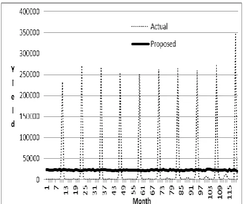
[image:4.595.302.549.322.509.2]The examples of the actual and the predicted values from the proposed model, in both fitting part (months 1- 108) and validation part (months 109-120), are shown in Fig. 9-11.
Fig. 9 Actual and predicted values in Loei province
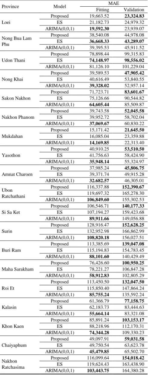
[image:4.595.304.549.548.753.2]Fig. 11 Actual and predicted values in Udon Thani province Using the MAE criteria, the performance of the proposed model compared to the simple exponential and ARIMA models is shown in Table 2. It can be seen that in the fitting part, the performance of the proposed model in most provinces seems to be slightly better than the simple exponential smoothing models, but slightly worse than the ARIMA models. For the validation part, the performance of the proposed model is superior to other models in all provinces except Nong Bua Lamphu and Udon Thani provinces.
IV. DISCUSSION
The LMM with CAR spatial effects for spatial time series data is proposed. It is attractive in the case that the spatial correlations can be accounted. It adopts the first law of geography stating that ―Everything is related to everything else, but near things are more related than distant things‖ [17]. The proposed model has a better performance compared to some common forecasting models—simple exponential smoothing and ARIMA. The limitation of our proposed model in this study is that the components of time series such as trend and seasonality are not considered, that is why we compared it with the simple exponential smoothing and ARIMA(0,0,1) models. Although the proposed model seems to be slightly inferior in the model fitting part, it has a better performance occurs in the validation part which are preferred. Likewise, the proposed model results the predicted values for all provinces at the same time, while simple exponential smoothing and ARIMA result them one province at the time. The proposed model can be applied to other spatial time series data.
V. CONCLUSIONS
The objective of this study is to propose an appropriate forecasting model to spatial time series data. The Bayesian inference in LMMs with CAR spatial effects is considered. The proposed model is applied to rice yield data in 19 Northeastern provinces of Thailand. The proposed model is the most superior, compared to the simple exponential smoothing and ARIMA models, especially in the validation part.
TABLE II
PERFORMANCE OF THE PROPOSED,ES, AND ARIMAMODELS
Province Model MAE
Fitting Validation
Loei
Proposed 19,663.52 23,324.83
ES 21,182.73 24,979.32
ARIMA(0,0,1) 19,592.30 23,939.07
Nong Bua Lam Phu
Proposed 38,540.08 44,978.08
ES 36,668.33 43,289.07
ARIMA(0,0,1) 39,395.53 45,911.52
Udon Thani
Proposed 78,898.44 99,315.83
ES 74,148.97 98,556.02
ARIMA(0,0,1) 81,126.10 101,229.04
Nong Khai
Proposed 39,589.53 47,905.42
ES 40,616.49 53,840.55
ARIMA(0,0,1) 39,328.02 52,957.14
Sakon Nakhon
Proposed 71,723.71 83,601.67
ES 75,126.66 90,544.82
ARIMA(0,0,1) 64,605.44 85,509.87
Nakhon Phanom
Proposed 39,743.58 52,045.58
ES 39,952.72 58,702.04
ARIMA(0,0,1) 37,069.67 60,830.22
Mukdahan
Proposed 15,171.42 21,645.50
ES 16,085.04 23,359.88
ARIMA(0,0,1) 14,169.85 22,313.40
Yasothon
Proposed 40,910.25 53,510.50
ES 41,756.63 58,424.90
ARIMA(0,0,1) 35,948.14 55,324.97
Amnat Charoen
Proposed 37,985.24 45,806.75
ES 39,371.74 49,915.28
ARIMA(0,0,1) 32.682.57 46,305.01
Ubon Ratchathani
Proposed 116,337.88 152,390.67
ES 119,697.32 165,278.30
ARIMA(0,0,1) 106,849.60 155,302.53
Si Sa Ket
Proposed 106,546.71 140,177.33
ES 107,194.27 159,423.68
ARIMA(0,0,1) 89,911.66 149,056.88
Surin
Proposed 128,916.47 152,628.25
ES 132,952.98 166,862.99
ARIMA(0,0,1) 108,820.18 156,027.51
Buri Ram
Proposed 113,385.69 139,047.08
ES 115,194.83 154,783.45
ARIMA(0,0,1) 88,101.60 140,429.49
Maha Sarakham
Proposed 76,426.60 100,950.25
ES 78,221.27 106,847.28
ARIMA(0,0,1) 58,912.83 102,805.29
Roi Et
Proposed 113,450.50 132,047.50
ES 115,850.40 147,864.24
ARIMA(0,0,1) 85,755.24 135,592.24
Kalasin
Proposed 61,366.79 77,158.75
ES 62,183.73 83,444.63
ARIMA(0,0,1) 55,664.14 83,321.08
Khon Kaen
Proposed 85,891.24 103,153.17
ES 88,218.96 112,170.31
ARIMA(0,0,1) 74,344.28 109,330.23
Chaiyaphum
Proposed 49,097.91 59,031.58
ES 49,750.54 63,623.78
ARIMA(0,0,1) 45,479.85 65,502.70
Nakhon Ratchasima
Proposed 116,099.64 154,018.42
ES 119,624.43 163,438.90
ARIMA(0,0,1) 103,443.75 164,380.28
ACKNOWLEDGMENT
REFERENCES
[1] Office of Agricultural Economics. (2012, October 5). Agricultural Production. Available: http://www.oae.go.th
[2] J. Besag, J. York, and A. Molli, ―Bayesian image restoration, with two applications in spatial statistics,‖ Annals of the Institute of Statistical Mathematics, vol. 43, pp. 1-21, 1991.
[3] L. Bernardinelli, D. Clayton, C. Pascutto, C. Montomoli, M. Ghislandi, and M. Songini, ―Bayesian analysis of space-time variation in disease risk,‖ Statistics in Medicine, vol. 14, pp. 2433-2443, 1995.
[4] D. Conway, C. Q. Li., J. Wolch, C. Kahle, and M. Jerrett, ―A spatial autocorrelation approach for examining the effects of urban greenspace on residential property values,‖ The Journal of Real Estate Finance and Economics, vol. 41, no. 2, pp. 150-169, 2010. [5] P. M. Yelland, ―Bayesian Forecasting of Part Demand,‖ International
Journal of Forecasting, vol. 26, pp. 374-396, 2010.
[6] P. Tongkhow, and N. Kantanantha, ―Bayesian models for time series with covariates, trend, seasonality, autoregression and outliers,‖
Journal of Computer Science, vol. 9, no. 3, pp. 291-298, 2013. [7] M. Diaconoa, A. Castrignanob, A. Troccolic, D. De Benedettob, B.
Bassod, and P. Rubino, ―Spatial and temporal variability of wheat grain yield and quality in a Mediterranean environment: A multivariate geostatistical approach,‖ Field Crops Research, vol. 131, pp. 49–62, 2012.
[8] B. T. West, K. B. Welch, and A. T. Galecki, Linear mixed models: A practical guide to using statistical software. New York: Chapman and Hall/CRC, 2007.
[9] J. Besag, ―Spatial Interaction and the Statistical Analysis of Lattice Systems,‖ Journal of the Royal Statistical Society Series B, vol. 36, no. 2, pp. 192–236, 1974.
[10] A. Maierbrugger. (2013, February 1). Thailand wants rice top spot back. Available: http://investvine.com/thailand-wants-rice-top-spot-back
[11] I. Nation. (2008, April 16). Rice strain is cause of comparatively low
productivity. Available:
http://nationmultimedia.com/2008/04/16/opinion/opinion_30070831. php
[12] N. M. F. Rahman, ―Forecasting of boro rice production in Bangladesh: An ARIMA approach,‖ Journal of the Bangladesh Agricultural University, vol. 8, no. 1, pp. 103–112, 2010.
[13] S. Banerjee, B. P. Carlin, and A. E. Gelfand. Hierarchical Modeling and Analysis for Spatial Data. Chapman and Hall/CRC Press. FL, 2004.
[14] P. Congdon, Bayesian Statistical Modelling. 2nd ed. New York: John Wiley and Sons, 2006.
[15] S. Geman and D. Geman, ―Stochastic Relaxation, Gibbs Distributions, and the Bayesian Restoration of Images,‖ IEEE Transactions of Pattern Analysis and Machine Intelligence, vol. 6, pp. 721-74, 1984.
[16] S. P. Brooks and G. O. Roberts, ―Assessing Convergence of Markov Chain Monte Carlo Algorithms,‖ Statistics and Computing, vol. 8, pp. 319-335, 1998.