Data Visualization for Constrained Data using
C
2
Rational Cubic Spline
Mohd Nain Hj Awang, Muhammad Abbas, Ahmad Abd Majid and Jamaludin Md Ali
Abstract—In this paper a rational cubic function in the form of cubic/quadratic, with three shape parameters has been developed. Data dependent sufficient constraints are derived for one of these shape parameter to preserve the shape of constrained data that is lying above the straight line. Remaining two of these shape parameters are left free for designer’s choice to refine the shape of the curves as desired. The shape preserving interpolating scheme is tested through different numerical examples and showing that the scheme is not only
C2
, local, computationally economical and visually pleasant but also guarantee the designer to refine the constrained curve as per industrial demand.
Index Terms—Shape preserving Interpolation, Rational cubic function, Constrained curves, Constrained data, Shape param-eters.
I. INTRODUCTION
S
Pline interpolation is a significant tool in Computer Graphics, Computer Aided Geometric Design and Engineering as well. Shape preserving of given data plays imperative role in the data visualization environment. Data visualization is the study of visual display of data. The main purpose of data visualization is a graphical representation of information in pretty effective and clear way. These graphical representations of data have great significance in many fields including engineering, military, education, art, medicine, advertising, transport, etc. Therefore, the user need to generate splines in these fields which can interpolate the data points in such a way that they preserve the inherited shape characteristics of data. Among the properties that the spline for curves and surfaces need to satisfy, smoothness and shape preservation of given data are mostly needed by all the designers.The cubic spline schemes have been used for quite a long time to deal with the problems of constructing smooth curves that passes through given data points. However, these splines sometimes fail to generate visually pleasing curves because of unwanted oscillations that are not suitable for design purposes. There arise many physical experiments where the data set is required to uphold some shape characteristics (constrained curve that is lying above the straight line, positivity, monotonicity and convexity). The designer is more interested in those interpolating schemes
Mohd Nain Hj Awang is with the School of Distance Education, Universiti Sains Malaysia, USM 11800 Pulau Pinang, Malaysia.
Muhammad Abbas is with the School of Mathematical Sciences, Universiti Sains Malaysia, USM 11800 Pulau Pinang, Malaysia, Corresponding’s Author E-mail: [email protected].
Ahmad Abd Majid is with the School of Mathematical Sciences, Univer-siti Sains Malaysia, USM 11800 Pulau Pinang, Malaysia.
Jamaludin Md Ali is with the School of Mathematical Sciences, Universiti Sains Malaysia, USM 11800 Pulau Pinang, Malaysia.
that carry these characteristics. Such ”shape-preserving interpolation” provide a chance to get rid of the undesirable oscillations that come across by using standard cubic spline interpolation and similar algorithms based on Hermite interpolation.
The traditional cubic spline scheme is failed to preserve the inherent shape feature like as the shape of data that is lying above the line as shown in the Fig. 1, Fig. 4 and Fig. 7. Since the traditional interpolating schemes merely depend on the data points, so just a change in data points can cause a modification or an alteration in the shape of curves. For this reason the need for some proficient shape preserving interpolating schemes arises which not only preserve the shape of the input data but also pay heed to the underlying smoothness of curves. In this paper such interpolating scheme is developed which not only provide the smoothness in the shape preserving curves but also control the shape of data everywhere.
In recent years, some work [1-11] has been published on shape preservation for shaped data. Abbas, et al [2] developed quadratic and cubic B´ezier interpolations constrained by a line. The author derived simple conditions on the middle points of quadratic and cubic B´ezier function to be constrained by a line. Abbas, et al [3] developed a piecewise rational cubic function with shape parameters to preserve the shape of constrained data. Simple data dependent conditions for shape parameter were derived to preserve the shape of data lying above the straight line. Brodlie, et al [4] constructed modified quadratic Shepard method which interpolates a scattered data of any dimension to preserve the positivity. The authors inserted extra knots in the interval in such a way that the desired shape of data was preserved. Brodlie, et al [5] developed a piecewise bi-cubic function arranged a data on rectangular mesh. They developed sufficient conditions on the first partial derivatives and mixed partial derivatives at the grid points to preserve the shape of surface data that was lying above the plane.
end points of cubic B´ezier function were left for user’s choice. Simple constraints were derived on two middle points of cubic B´ezier function constrained by a circle, an ellipse and straight line with point of intersection. Furthermore, the cubic B´ezier function represented the S-shaped and C-S-shaped curves. Goodman, et al [9] developed two schemes of interpolating to preserve the shape of data lying on one side of the straight line by rational cubic functions. Firstly, they preserved the shape of data lying above the straight line by scaling the weights by some scale factor. Secondly, the authors preserved the shape of data by the insertion of new interpolating point. Jeok, et al [11] developed C1 monotonicity and G1 constrained curve which was lie on the same side of given constraint line using cubic B´ezier-like function.
This paper is a contribution towards the advancements in the existing schemes. So new technique has proposed in this progress. The technique used in this paper has many prominent features.
1) The smoothness of newly developed interpolant isC2 while in [3], [4], [5], [9], the degree of smoothness is
C1.
2) Experimental evidence suggest that the scheme is not only computationally economical but also produce smoother graphical results as compared to existing scheme [3].
3) In [7], the authors developed schemes that work for equally spaced data while the scheme developed in this paper works for both equally and unequally spaced data.
4) In [4], [5], the authors developed the scheme to achieve the desired shape of data by inserting extra knots be-tween any two knots in the interval while we preserve the shape of data by only imposing constraints on free parameters without any extra knots.
5) The proposed scheme is computationally economical and time saving because there exists only one tri-diagonal system of linear equations for finding the values of derivative parameters.
This paper is organized as follows: In section II, a newC2 piecewise rational cubic function with three shape parame-ters which are used in its presentation is developed. Data dependent sufficient conditions are derived for single shape parameter to preserve the shape of data that is lying above the line is given in section III. Sufficient numerical examples are given in subsection III-A to prove the worth of the scheme. The concluding remarks are presented to end the paper.
II. RATIONALCUBICSPLINEFUNCTION
Let {(xi, fi) : i= 0,1,2, ..., n} be the given set of data
points such that x0 < x1 < x2 < ... < xn. A piecewise
rational cubic function with three shape parameters in each subinterval Ii = [xi, xi+1], i= 0,1,2, ...., n−1 is defined as:
S(x) =Si(x) =
∑3
i=0(1−θ) 3−iθiξ
i qi(θ)
(1)
with,hi=xi+1−xi, θ= x−xi
hi
, θ∈[0,1]
and
ξ0=uifi
ξ1=fi(2ui+vi+wi) +uihidi ξ2=fi+1(ui+ 2vi+wi)−vihidi+1
ξ3=vifi+1
qi(θ) = (1−θ)2ui+θ(1−θ) (wi+ui+vi) +θ2vi
(2) whereui, vi, wi are the positive shape parameters that are
used to control the shape of interpolating curve and provide the designer liberty to refine the curve as desired. Let di
denotes the derivative value at knots xi that is used for the
smoothness of curve. LetS′(x) andS′′(x) denote the first and second ordered derivatives with respect tox.
The following interpolatory conditions are imposed for the
C2continuity of the piecewise rational cubic function (1),
S(xi) =fi, S(xi+1) =fi+1
S′(xi) =di, S′(xi+1) =di+1
S′′(xi+) = S′′(xi−), i= 1,2, ..., n−1
(3)
From equation (3), theC2 interpolating conditions produce the following system of linear equations
αidi−1+δidi+γidi+1=λi (4)
with,
αi=uiui−1hi
δi=hiui(ui−1+vi−1+wi−1) +hi−1vi−1(ui+vi+wi) γi=vivi−1hi−1
λi=vi−1hi−1(ui+ 2vi+wi)∆i
+uihi(2ui−1+vi−1+wi−1)∆i−1
(5) and∆i= (fi+1−fi)/hi.
TheC2piecewise rational cubic function (1) is reformulated after using equation (2) as:
S(xi) = pi(θ) qi(θ)
(6)
with,
pi(θ) =
uifi(1−θ)3+
(fi(2ui+vi+wi) +uihidi) θ(1−θ)2+
(fi+1(ui+ 2vi+wi)−vihidi+1)θ2(1−θ)+ vifi+1θ3
qi(θ) = (1−θ)2ui+θ(1−θ) (wi+ui+vi) +θ2vi
Remark 1: The system of linear equations defined in equation (4) is a strictly tri-diagonal and has a unique solution for the derivatives parametersdi, i= 1,2, ..., n−1
for all ui, vi >0 and wi ≥ 0. Moreover, it is efficient to
apply LU decomposition method to solve the system for the values of derivatives parametersd′is.
Remark 2: To make the rational cubic function smoother,
C2continuity is applied at each knot. The system (4) involves
n−1 linear equations while unknown derivative values are
n + 1. So, two more equations are required for unique solution. For this, we impose end conditions at end knots as:
Remark 3: For the values of shape parameters set as:
ui = 1, vi = 1 and wi = 0 in each
subinter-valIi= [xi, xi+1], i= 0,1,2, ...., n−1, the rational cubic
function reduces to standard cubic Hermite spline.
III. SHAPEPRESERVINGCONSTRAINEDC2RATIONAL CUBICCURVEINTERPOLATION
In this section, we discuss the problem of shape preserving rational cubic constrained curve that lies above the straight line. TheC2piecewise rational cubic function (6) with three shape parameters values taken as: ui = 1, vi = 1 and wi = 0 does not preserve the inherited shape features of
constrained data because the interpolant reduces to standard cubic Hermite spline. This requires to impose suitable con-straints on the shape parameters to preserve the shape of constrained data that lies above the straight line.
Let{(xi, fi) :i= 0,1,2, ..., n}be given data set lying above
the straight liney=mx+c i.e.
fi> mxi+c, ∀i= 0,1,2, ..., n (8)
where m and c is the slope and y-intercept of the line respectively.
The curve of the given set of data points lies above the straight line if the C2 rational cubic function (6) holds the following condition
S(x)> y ∀x∈[x0, xn] (9)
In each subinterval Ii= [xi, xi+1], the relation (9) can be
expressed as:
Si(x) = pi(θ) qi(θ)
> mxi+c (10)
The equation of straight line in parameter θis defined as:
ri(1−θ) +siθ, θ∈[0,1] (11)
where,
ri=mxi+candsi=mxi+1+c. The parametric form of equation (10) is
Si(x) = pi(θ) qi(θ)
> ri(1−θ) +siθ, i= 0,1,2, ..., n (12)
or
Si(x) = pi(θ) qi(θ)−
ri(1−θ) +siθ >0 (13)
Multiply both sides of equation (13) byqi(θ), we have
Fi(x) =
3
∑
k=0
(1−θ)3−kθkHk,i (14)
where,
H0,i= (fi−ri)ui
H1,i= (fi−ri)(ui+vi) + (fi−ri)wi−ui(si−dihi−fi) H2,i= (fi+1−si)(ui+vi) + (fi+1−si)wi
−vi(ri+di+1hi−fi+1) H3,i= (fi+1−si)vi
Necessary conditions derived from equation (8) are:
{
(fi−ri)>0
(fi+1−si)>0
(15)
The polynomialFi(x)>0if Hk,i>0, k= 0,1,2,3.
Since ui, vi>0 and from equation (15), it is obvious that
H0,i>0andH3,i>0. H1,i>0if
wi>
ui(si−dihi−fi)
(fi−ri)
(16)
H2,i>0if
wi>
vi(ri+di+1hi−fi+1) (fi+1−si)
(17)
The above results can be summarized as:
Theorem 3.1: TheC2piecewise rational cubic function
S(x), defined over the each subintervalIi= [xi, xi+1] , in (6), preserves the shape of data that lies above the straight line, if the following sufficient conditions are satisfied.
ui>0, vi>0, wi> max
{
0,ui(si−dihi−fi)
(fi−ri)
,vi(ri+di+1hi−fi+1)
(fi+1−si)
}
(18) The above constraints can be rewritten as:
ui>0, vi>0,
wi=pi+max
0,ui(si−dihi−fi)
(fi−ri) ,
vi(ri+di+1hi−fi+1)
(fi+1−si)
, pi>0.
(19)
A. Numerical Examples
Example 1: In Table I which is borrowed from [1], con-strained data sets is taken that lie above the straight line
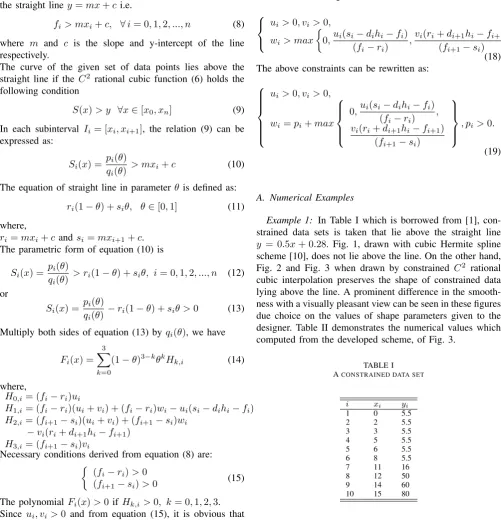
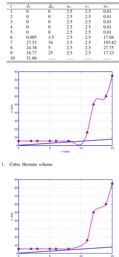
[image:3.595.47.549.266.787.2]y = 0.5x+ 0.28. Fig. 1, drawn with cubic Hermite spline scheme [10], does not lie above the line. On the other hand, Fig. 2 and Fig. 3 when drawn by constrained C2 rational cubic interpolation preserves the shape of constrained data lying above the line. A prominent difference in the smooth-ness with a visually pleasant view can be seen in these figures due choice on the values of shape parameters given to the designer. Table II demonstrates the numerical values which computed from the developed scheme, of Fig. 3.
TABLE I ACONSTRAINED DATA SET
i xi yi
1 0 5.5
2 2 5.5
3 3 5.5
4 5 5.5
5 6 5.5
6 8 5.5
7 11 16
8 12 50
9 14 60
NUMERICAL RESULTS OFFIG. 3
i di ∆i ui vi wi
1 0 0 2.5 2.5 0.01
2 0 0 2.5 2.5 0.01
3 0 0 2.5 2.5 0.01
4 0 0 2.5 2.5 0.01
5 0 0 2.5 2.5 0.01
6 0.005 3.5 2.5 2.5 17.04
7 27.53 34 2.5 2.5 195.82
8 24.38 5 2.5 2.5 27.75
9 16.77 25 2.5 2.5 17.23
10 31.66 ... ... ... ...
0 5 10 15
0 10 20 30 40 50 60 70 80 90
x−axis
[image:4.595.60.266.70.515.2]y−axis
Fig. 1. Cubic Hermite scheme
0 5 10 15
0 10 20 30 40 50 60 70 80 90
x−axis
[image:4.595.46.547.104.760.2]y−axis
Fig. 2. ConstrainedC2rational cubic interpolation withu
i= 0.25, vi=
0.25
0 5 10 15
0 10 20 30 40 50 60 70 80 90
x−axis
[image:4.595.80.258.573.716.2]y−axis
Fig. 3. ConstrainedC2 rational cubic interpolation withu
i= 2.5, vi=
2.5
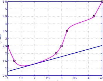
Example 2: A constrained data set is taken in Table III that lie above the straight line y = 0.5x+ 0.28. Fig. 4, generated by cubic Hermite spline scheme [10], does not lie above the line. On the other hand, Fig. 5 and Fig. 6 when drawn by constrained C2 rational cubic interpolation preserves the shape of constrained data lying above the line. A remarkable difference in the smoothness with a visually pleasant view can be seen in these figures due choice on the values of shape parameters given to the designer. Table IV demonstrates the numerical values which computed from the developed scheme, of Fig. 6.
TABLE III CONSTRAINED DATA SET
i 1 2 3 4 5 6 7
xi 1 1.25 2.8 3 3.2 4.2 4.5
yi 2.5 1.5 2 2.5 3.5 4.5 5.5
TABLE IV
NUMERICAL RESULTS OFFIG. 6
i 1 2 3 4 5 6 7
di -4.60 -3.24 1.78 4.01 4.64 2.16 3.87
∆i -4.0 0.32 2.5 5.0 1.0 3.33 ...
ui 0.75 0.75 0.75 0.75 0.75 0.75 ...
vi 0.75 0.75 0.75 0.75 0.75 0.75 ...
wi 3.5 3.56 25.67 4.74 6.95 5.53 ...
1 1.5 2 2.5 3 3.5 4 4.5 0.5
1 1.5 2 2.5 3 3.5 4 4.5 5 5.5
x−axis
y−axis
1 1.5 2 2.5 3 3.5 4 4.5 0.5
1 1.5 2 2.5 3 3.5 4 4.5 5 5.5
x−axis
[image:5.595.329.517.76.415.2]y−axis
Fig. 5. ConstrainedC2rational cubic curve withu
i= 0.25, vi= 0.25
1 1.5 2 2.5 3 3.5 4 4.5 0.5
1 1.5 2 2.5 3 3.5 4 4.5 5 5.5
x−axis
[image:5.595.79.256.257.397.2]y−axis
Fig. 6. ConstrainedC2rational cubic curve withu
i= 0.75, vi= 0.75
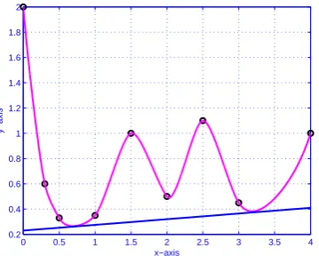
Example 3: A constrained positive data set in Table V demonstrates the velocity of wind which is noted in different time interval. The velocity is inherently constrained positive that lies above the straight line y = 0.5x+ 0.28 and we therefore, require a C2 rational cubic function with shape parameters to preserve this shape characteristic. The x-values are time (min) and f-values are velocity of wind (km/min). Fig. 7 is produced by cubic Hermite spline scheme [10] that does not maintain the shape of constrained positive data which is the imperfection of this spline. Fig. 8 and Fig. 9 are produced by constrainedC2 rational cubic interpolation preserve the shape of constrained positive data that lies above the straight line. Fig. 9 is more visually pleasing and smooth as compared to Figure 8 due to different values of shape parameters. Table VI represents the computed values from the developed scheme of Fig. 9.
TABLE V
A 2DCONSTRAINED DATA SET
i xi yi
1 0.0 2.0
2 0.3 0.6
3 0.5 0.33
4 1.0 0.35
5 1.5 1.0
6 2.0 0.5
7 2.5 1.1
8 3.0 0.45
9 4.0 1.0
TABLE VI
NUMERICAL RESULTS OFFIG. 9
i di ∆i ui vi wi
1 -6.65 -4.66 2.5 2.5 3.50
2 -2.56 -1.35 2.5 2.5 3.50
3 -0.97 0.04 2.5 2.5 4.34
4 0.67 1.30 2.5 2.5 3.50
5 0.21 -1.00 2.5 2.5 3.50
6 -0.74 1.20 2.5 2.5 3.50
7 0.05 -1.30 2.5 2.5 3.50
8 -0.87 0.55 2.5 2.5 3.81
9 1.78 .... .... .... ....
0 0.5 1 1.5 2 2.5 3 3.5 4 0.2
0.4 0.6 0.8 1 1.2 1.4 1.6 1.8 2
x−axis
y−axis
Fig. 7. Cubic Hermite scheme
0 0.5 1 1.5 2 2.5 3 3.5 4 0.2
0.4 0.6 0.8 1 1.2 1.4 1.6 1.8 2
x−axis
y−axis
Fig. 8. ConstrainedC2rational cubic interpolation withu
i= 0.25, vi=
0.25
IV. CONCLUDINGREMARKS
[image:5.595.332.514.418.564.2]0 0.5 1 1.5 2 2.5 3 3.5 4 0.2
0.4 0.6 0.8 1 1.2 1.4 1.6 1.8 2
x−axis
[image:6.595.79.259.61.205.2]y−axis
Fig. 9. ConstrainedC2 rational cubic interpolation withu
i= 2.5, vi=
2.5
knots were inserted between any two knots in the interval where the interpolant loses the desired shape of the data while we obtain the desired shape of the data without any additional knots. In this paper, there exists only one tri-diagonal system of linear equations for finding the values of derivative parameters which is computational economical.
The interpolating scheme developed in this paper is C2, smoother, local, computationally economical and visually pleasing. The proposed scheme works for both equally and unequally spaced data while the schemes developed in [7] work for only equally spaced data. Experimental evidence suggest that the proposed C2 rational cubic interpolation appear to produce smoother graphical results. In future, the authors are interested to extend the C2 rational cubic function to rational bi-cubic function and bi-cubic partially blended rational function to solve the C2 shape preserving interpolating surface problem in rectangular case.
ACKNOWLEDGMENT
The authors are grateful to the anonymous referees for their helpful, valuable comments and suggestions in the improvement of this manuscript. This work was supported by School of Mathematical Sciences and School of Distance Education, Universiti Sains Malaysia and Government of Malaysia. The second author does acknowledge University of Sargodha, Sargodha Pakistan for the financial support.
REFERENCES
[1] Akima, H. (1970), ”A new method of interpolation and smooth curve fitting based on local procedures”, Journal of the Association for Computing Machinery 17, pp. 589-602.
[2] Abbas, M., Jamal, E., and Ali, J. M. (2011), ”B´ezier curve interpolation constrained by a line”, Applied Mathematical sciences, 5(37), pp. 1817-1832.
[3] Abbas, M., Majid, A. A., and Ali, J. M. (2012), ”Shape preserving constrained data visualization using spline functions”, International journal of Applied Mathematics & Statistics 29 (5), pp. 34-50. [4] Brodlie, K. W., Asim, M. R., and Unsworth, K. (2005), ”Constrained
visualization using Shepard interpolation family”, Computers and Graphics forum 24(4), pp. 809-820.
[5] Brodlie,K. W. and Mashwama,P. and Butt,S. (1995), ”Visualization of surface data to preserve positivity and other simple constraints”, Computers and Graphics 4(19), pp. 585–594.
[6] Costantini, P. (1997), ”Boundary-valued shape preserving interpolating splines”, ACM Transactions on Mathematical Software (TOMS) 23(2), pp. 229-251.
[7] Duan, Q., Wang, L. and Twizell, E. H. (2005), ”A newC2 rational interpolation based on function values and constrained control of the interpolant curves”, Journal of Applied Mathematics and Computation 61, pp. 311-322.
[8] Fuziatul, N. A. S., Abbas, M., Uzma, B., Nain, M. H. A., Jamal, E.and Ali, J. M. (2012), ”Cubic B´ezier Constrained Curve Interpolation”, J. Basic. Appl. Sci. Res. 2(4), pp. 3682-3692.
[9] Goodman, T. N. T., Ong, B. H., and Unsworth, K. (1991), ”Constrained interpolation using rational cubic splines”. In NURBS for Curve and Surface Design (Farin, G., ed.), Philadelphia, SIAM, pp. 59-74. [10] Hoschek, J. and Lasser, D. (1993), ”Fundamentals of Computer Aided
Geometric Design”, translated by L.L. Schumaker. Massachusetts: A K Peters, Wellesley.