A Simplified Binary Artificial Fish Swarm
Algorithm for Uncapacitated Facility
Location Problems
Md. Abul Kalam Azad, Member, IAENG, Ana Maria A.C. Rocha and Edite M.G.P. Fernandes
Abstract—Uncapacitated facility location problem (UFLP) is a combinatorial optimization problem, which has many applications. The artificial fish swarm algorithm has recently emerged in continuous optimization problem. In this paper, we present a simplified binary version of the artificial fish swarm algorithm (S-bAFSA) for solving the UFLP. In S-bAFSA, trial points are created by using crossover and mutation. In order to improve the quality of the solutions, a cyclic reinitialization of the population is carried out. To enhance the accuracy of the solution, a local search is applied on a predefined number of points. The presented algorithm is tested on a set of benchmark uncapacitated facility location problems.
Index Terms—Uncapacitated facility location, 0–1 program-ming, artificial fish swarm algorithm, local search.
I. INTRODUCTION
T
HE artificial fish swarm algorithm (AFSA) is one of the recent population-based stochastic methods that has appeared for solving continuous and engineering design optimization problems [1], [2], [3], [4]. When applying to an optimization problem, a ‘fish’ represents an individual point in a population. The algorithm simulates the behavior of a fish swarm inside water. At each iteration, trial points are generated from the current ones using either a chasing behav-ior, a swarming behavbehav-ior, a searching behavior or a random behavior. Each trial point competes with the corresponding current and the one with best fitness is passed to the next iteration as current point. There are different versions and hybridizations of AFSA available in [5], [6], [7].The most widely studied location problems available in the literature are combinatorial optimization problems and NP-hard. We are interested about the uncapacitated facility location problem (UFLP). The UFLP involves a set of customers with known demands and a set of alternative candidate facility locations. If a candidate location is to be selected for open a facility, a known fixed setup cost will be incurred. Moreover, there is also a fixed known delivery cost from each candidate facility location to each customer. The goal of UFLP is to connect each customer to exactly one opened facility in the way that the sum of all associated costs (setup and delivery) is minimized. It is assumed that the facilities have sufficient capacities to meet all customer demands connected to them. The UFLP is used to model Manuscript received March 05, 2013; revised April 07, 2013. M. A. K. Azad acknowledges Ciˆencia 2007 of FCT (Foundation for Science and Technology), Portugal for the fellowship grant: C2007-UMINHO-ALGORITMI-04. Financial support from FEDER COMPETE (Operational Programme Thematic Factors of Competitiveness) and FCT under project: FCOMP-01-0124-FEDER-022674 is also acknowledged.
Algoritmi R&D Centre, School of Engineering, University of Minho, 4710-057 Braga, Portugal. e-mail:{akazad,arocha,emgpf}@dps.uminho.pt
many applications such as bank account allocation, clustering analysis, location of offshore drilling platforms, economic lot sizing, machine scheduling, portfolio management, design of communication networks, etc.
Let in the UFLP, the number of alternative candidate facility locations be m and the number of customers be n. The mathematical formulation of the UFLP is given as follows:
minimizez(x,y)≡
m
X
i=1
n
X
j=1
cijxij+ m
X
i=1 fiyi
subject to
m
X
i=1
xij= 1, for allj
xij≤yi for alli, j
xij, yi∈ {0,1} for alli, j,
(1)
where
cij =the delivery cost of meeting customerj’s
demand from facility at locationi;
fi =the setup cost of facility at locationi;
xij =
1 if customer j is served from locationi,
0 otherwise;
yi =
1 if a facility is opened at location i,
0 otherwise.
It is noted that xij is a binary variable (0/1 bit) since the
demand of customer j, j = 1, . . . , n, is fulfilled by exactly one facility, (i.e. no partial fulfillment of demand is allowed) sayk, in which casexkj= 1,xij = 0,i= 1, . . . , m,i6=k.
yi is also a binary variable since a facilityiis either opened
(yi= 1), in which case the fixed setup costfi is incurred, or
it is not opened (yi= 0) and no fixed setup cost is incurred.
in a continuous particle swarm optimization algorithm, PSO with local search [18].
This paper presents a binary version of AFSA for solving the uncapacitated facility location problem (1). A previous binary version of AFSA, denoted by bAFSA, is presented in [19], where a set of small 0–1 multidimensional knapsack problems were successfully solved. To create the trial points from the current ones in a population, bAFSA chooses each point/fish behavior according to the number of points inside its ‘visual scope’, i.e., inside a closed neighborhood centered at the point. To identify those points, the Hamming distance between pairs of points is used.
For instance, the chasing behavior is chosen when the ‘visual scope’ is assumed to be not crowded. In terms of fish behavior, this happens when a fish, or a group of fish in the swarm, discover food and the others find the food dangling quickly after it. The bAFSA creates the trial point after a uniform crossover between the individual point and the best point inside the ‘visual scope’ is performed.
Alternatively, when swimming, fish naturally assembles in groups which is a living habit in order to guarantee the existence of the swarm and avoid dangers. This is a swarming behavior and the ‘visual scope’ is also assumed to be not crowded. Here, a uniform crossover between the individual point and the central point of the ‘visual scope’ is performed to create the trial point.
The searching behavior occurs when fish discovers a region with more food, by vision or sense, going directly and quickly to that region. This behavior assumes that the ‘visual scope’ is crowded. The trial point is created by performing a uniform crossover between the individual point and a randomly chosen point from the ‘visual scope’.
Finally, in the random behavior, a fish with no other fish in its neighborhood to follow, moves randomly looking for food in another region. This happens when the ‘visual scope’ is empty and the trial point is created by randomly setting a binary string of 0/1 bits.
Past experience has shown that the computational effort of computing the ‘visual scope’ of each individual and checking the points that are inside the ‘visual scope’, along all itera-tions, increases enormously with the number of variables.
The purpose of the herein presented study is to reduce the computational requirements, in terms of number of iterations and execution time, to reach the optimal solution. The procedures that are used to choose which behavior is to be performed to each current point in order to create the corresponding trial point are simplified. Thus, a simplified binary version of AFSA, henceforth denoted by S-bAFSA, is produced. Briefly, for all points of the population, except the best, random, searching and chasing behavior are randomly chosen using two target probability values0< τ1< τ2<1,
and uniform crossover is performed to create the trial points. A simple 4-flip mutation is performed in the best point of the population to generate the corresponding trial point. To improve the accuracy of the solutions obtained by the algorithm, a swap move local search adapted from [17] and a cyclic reinitialization of the population are implemented. A benchmark set of uncapacitated facility location problems is used to test the performance of the S-bAFSA.
The organization of this paper is as follows. The proposed simplified binary version of AFSA is described in Section II.
Section III describes the experimental results and finally we draw the conclusion of this study in Section IV.
II. THEPROPOSEDS-BAFSA
In bAFSA [19], each trial point is created from the current one by using the original concept of ‘visual scope’ of a point. To identify the points inside the ‘visual scope’ of each individual point, the Hamming distance is used. For points of equal bits length, this distance is the number of positions at which the corresponding bits are different. The computational requirement of this procedure grows rapidly with problem’s dimension. Furthermore, in some cases the population stagnates and the algorithm converges to a non-optimal solution.
To overcome these drawbacks, the herein presented S-bAFSA will not make use of the concept of ‘visual scope’ of an individual point, will select each fish/point behavior on the basis of two user defined target probability values and will not perform the swarming behavior ever, since the central point may not depict the center of the distribution of solutions. Furthermore, to be able to reach the solution with high accuracy and avoid convergence to a non-optimal solution, a simple local search and a random reinitialization of the population are performed.
Details of the proposed S-bAFSA to solve the uncapac-itated facility location problem (1) are described in the following. The first step of S-bAFSA is to design a suitable representation scheme of a current point in a population for solving the UFLP. Since the facilities are to be opened or not at candidate locations, a current point y= (y1, y2, . . . , ym)
is represented by a binary string of 0/1 bits of length m. At initial iteration/generation N individual points, yl, l =
1, . . . , N, in a population are randomly generated [19], [20]. We note that the maximum population size N of binary strings of 0/1 bits of lengthmis2m.
When the locations of facilities to be opened are deter-mined, i.e., after initializing a current pointyl, the optimal
connection of customers will be obtained easily. Indeed, each customer j is connected by the facility opened at location k (with bit 1) whose delivery cost ckj is minimal
(k= arg min
i=1,...,m{cij}). Then x l
kj = 1 and x l
ij = 0, i =
1, . . . , m; i 6= k. Then, the objective function z(xl,yl) is
evaluated and this is the facility location decision that should be done optimally.
A. Generating Trial Points in S-bAFSA
After initializing current points yl, l = 1, . . . , N and
connecting customers to opened facilitiesxl, crossover and
mutation are performed to create trial points,vlbased onyl
in successive iterations by using the fish behavior of random, searching and chasing. We introduce the probabilities 0 < τ1< τ2<1 in order to perform the movements of random,
searching and chasing. The fish behavior in S-bAFSA that create the trial points are outlined as follows.
The random behavior is implemented when a uniformly distributed random numberrand(0,1) is less than or equal to τ1. In this behavior the trial point vl is created by
randomly setting 0/1 bits of lengthm.
The chasing behavior is implemented whenrand(0,1)≥
found so far in the population,ybest. Here, the trial pointvl
is created using a uniform crossover between yl andybest.
In uniform crossover, each bit of the trial point is created by copying the corresponding bit from one or the other current point with equal probability.
The searching behavior is related to the movement towards a point yrand where ‘rand’ is an index randomly chosen
from the set{1,2, . . . , N}. This behavior is implemented in S-bAFSA when τ1< rand(0,1)< τ2. A uniform crossover
betweenylandyrandis performed to create the trial pointvl.
In S-bAFSA, the three fish behavior previously described are implemented to create N−1 trial points; the best point
ybest is treated separately. A mutation is performed in the
pointybest to create the corresponding trial pointv. In
mu-tation, a 4-flip bit operation is performed, i.e., four positions are randomly selected and the bits of the corresponding positions are changed from 0 to 1 or vice versa.
After creating the trial point vl, the optimal connection
of customers corresponding to this vl (opened facility),ul,
is done according to the procedure described above for l= 1, . . . , N and then the objective function is evaluated.
B. Selection of the New Population
At each iteration, each trial point vl and corresponding ulcompetes with the current pointyland correspondingxl,
in order to decide which one should become a member of the population in the next iteration. Hence, if z(ul,vl) ≤ z(xl,yl), then the trial point becomes a member of the
population in the next iteration, otherwise the current point is preserved to the next iteration.
C. Local Search
A local search is often important to improve a current solution. It searches for a better solution in the neighborhood of the current solution. If such solution is found then it replaces the current solution. In S-bAFSA, we implement a simple local search based on swap move [17] after the selection procedure. In this local search, the swap move changes the value of a 0 bit of a current point to 1 and simultaneously another 1 bit to 0, so that the total number of opened facilities does not change. Here, the local search method has two parameters: Nloc (=τ3N, τ3 ∈(0,1)), the
number of current points selected randomly from the popula-tion to perform local search andmswap (=τ4Nbit 0(number
of 0 bits in a current point, yl), τ4∈(0,1)), the number of
positions selected randomly in a point to perform the swap move. After performing the local search, the new optimal connection of customers to the new opened facilities is made. Then the new points become members of the population if they improve the objective function value with respect to the corresponding current points.
The pseudocode of the local search used in S-bAFSA is shown in Algorithm 1.
D. Reinitialization of the Population
While testing bAFSA [19], it was noticed that, in some cases, the points in a population converged to a non-optimal point. To diversify the search, we propose to reinitialize the population randomly, every R iterations keeping the best solution found so far. In practical terms, this technique has greatly improved the quality of the solutions.
Algorithm 1 Local search
Require: the values of parametersτ3 andτ4 1: ComputeNloc=int(τ3N)
2: Randomly select Nloc points i.e.yr, r = 1, . . . , Nloc from current
population
3: forr= 1toNlocdo
4: Setsr:=yr,zr:=z(xr,yr)and computeNbit 0
5: Computemswap=int(τ4Nbit 0) 6: ifmswap>0then
7: fori= 1tomswapdo
8: Perform swap move onsr to createsrβ
9: Determine optimal connection of srβ, xrβ, and set zβ :=
z(xrβ,srβ)
10: ifzβ< zrthen
11: Setsr := srβ and replace corresponding connection and objective function value
12: end if
13: end for
14: end if
15: end for
E. The Algorithm
The proposed S-bAFSA terminates when the minimum objective function value reaches the known optimal value within a toleranceǫ >0, or a maximum number of iterations is exceeded, i.e., when
t > Tmax or |zbest−zopt| ≤ǫ (2)
holds, where Tmax is the allowed maximum number of
iterations, zbest is the minimum objective function value attained at iteration t and zopt is the known optimal value available in the literature. However, when the optimal value of the problem is not known, the algorithm may use other termination conditions. The pseudocode of S-bAFSA for solving the uncapacitated facility location problem (1) is shown in Algorithm 2.
Algorithm 2 S-bAFSA
Require: Tmaxandzoptand other values of parameters
1: Sett:= 1. Initialize populationyl, l= 1,2, . . . , N
2: Determine optimal connection, evaluate them and identify(xbest,ybest)
andzbest
3: while ‘termination conditions are not met’ do 4: if MOD(t, R) = 0then
5: Reinitialize populationyl, l= 1,2, . . . , N−1
6: Determine optimal connection, evaluate them and identify
(xbest,ybest)andzbest
7: end if
8: forl= 1toN do
9: ifl=best then
10: Perform 4-flip bit mutation to create trial pointvl
11: else
12: ifrand(0,1)≤τ1 then
13: Perform random behavior to create trial pointvl
14: else ifrand(0,1)≥τ2then
15: Perform chasing behavior to create trial pointvl
16: else
17: Perform searching behavior to create trial pointvl
18: end if
19: end if
20: end for
21: Determine optimal connection ul for vl, l = 1,2, . . . , N and
evaluate them
22: Select the population of next iteration(xl,yl),l= 1,2, . . . , N
23: Perform local search 24: Identify(xbest,ybest)andzbest
25: Sett:=t+ 1
TABLE I
COMPARATIVE RESULTS OF MDE1,MDE2ANDS-BAFSA
mDE1 mDE2 S-bAFSA
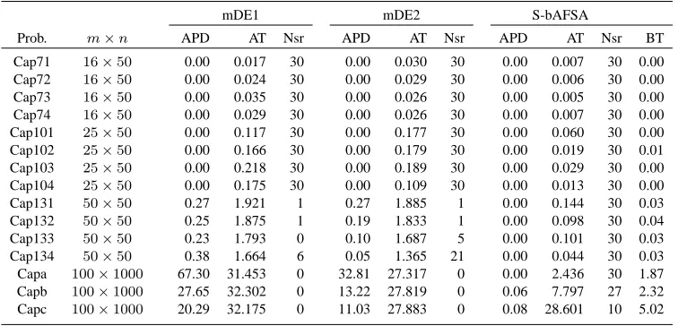
Prob. m×n APD AT Nsr APD AT Nsr APD AT Nsr BT Cap71 16×50 0.00 0.017 30 0.00 0.030 30 0.00 0.007 30 0.00 Cap72 16×50 0.00 0.024 30 0.00 0.029 30 0.00 0.006 30 0.00 Cap73 16×50 0.00 0.035 30 0.00 0.026 30 0.00 0.005 30 0.00 Cap74 16×50 0.00 0.029 30 0.00 0.026 30 0.00 0.007 30 0.00 Cap101 25×50 0.00 0.117 30 0.00 0.177 30 0.00 0.060 30 0.00 Cap102 25×50 0.00 0.166 30 0.00 0.179 30 0.00 0.019 30 0.01 Cap103 25×50 0.00 0.218 30 0.00 0.189 30 0.00 0.029 30 0.00 Cap104 25×50 0.00 0.175 30 0.00 0.109 30 0.00 0.013 30 0.00 Cap131 50×50 0.27 1.921 1 0.27 1.885 1 0.00 0.144 30 0.03 Cap132 50×50 0.25 1.875 1 0.19 1.833 1 0.00 0.098 30 0.04 Cap133 50×50 0.23 1.793 0 0.10 1.687 5 0.00 0.101 30 0.03 Cap134 50×50 0.38 1.664 6 0.05 1.365 21 0.00 0.044 30 0.03 Capa 100×1000 67.30 31.453 0 32.81 27.317 0 0.00 2.436 30 1.87 Capb 100×1000 27.65 32.302 0 13.22 27.819 0 0.06 7.797 27 2.32 Capc 100×1000 20.29 32.175 0 11.03 27.883 0 0.08 28.601 10 5.02
III. EXPERIMENTALRESULTS
We code S-bAFSA in C and compile with Microsoft Visual Studio 10.0 compiler in a PC having 2.5 GHz Intel Core 2 Duo processor and 4 GB RAM. We consider 15 benchmark uncapacitated facility location problems available in OR-Library [21]. Among them, Cap71–Cap74 are small size problems, Cap101–Cap104 and Cap131–Cap134 are medium size problems and the other three Capa–Capc are large size problems. It is worth mentioning that the names of the problems are the originally used in OR-Library. We setN = 100,Tmax= 1000andǫ= 10−
4
. We set R= 100 for the reinitialization of the population and τ1 = 0.1, τ2 = 0.9,τ3 = 0.1 andτ4 = 0.25 after performing several
experiments. Thirty independent runs were carried out with each problem.
Firstly, we compare S-bAFSA with two binary versions of the modified differential evolution algorithm (mDE) pre-sented in [22]. The differential evolution algorithm was originally presented in [23] to solve continuous global opti-mization problems. In [22], a modified mutation is presented. First a linear convex combination of two mutant points is implemented: one comes from the usual DE/rand/1 strategy and the other from a DE/rand/1 case where the base point is the best of the three randomly chosen points. Second, the best point found so far is cyclically used as the base point to create the mutant point at those iterations. The two binary versions of the mDE are herein denoted by mDE1 and mDE2. In mDE1, current points in a population are initialized randomly by setting 0/1 bits and mutation is performed according to [22]. After performing mutation, the continuous components of a point are transformed into 0/1 bits of a binary string according to the procedure described in [24]. This procedure determines the probabilities of components in a continuous point. These probabilities are then taken into account to transform a continuous point into a binary string. Suppose,
gi, i= 1, . . . , mis a continuous point; then each component
gi is transformed intoyi in the following way
yi=
1 ifrand(0,1)< sig(gi)
0 otherwise,
wheresig(gi)is the sigmoid limiting function expressed by
sig(gi) =
1 1 +e−gi.
On the other hand, in mDE2, current points are initialized within the bounds (0,10.0) and mutation is performed ac-cordingly. Then the continuous current points and mutant points are transformed into binary strings of 0/1 bits accord-ing to the transformation procedure described in [18]. The therein presented procedure transforms each componentgiof
a continuous point intoyi, fori= 1, . . . , min the following
way
yi=⌊|gimod2|⌋ (3)
where⌊·⌋ represents the floor function. All the other steps of the mDE algorithm are performed similarly to those described in [22].
We also code variants mDE1 and mDE2 in C. We also set N = 100, Tmax = 1000 and ǫ = 10−
4
. Other values of the parameters are set according to [22]. Here, 30independent runs were also carried out. The comparative results are shown in Table I. The performance criteria among 30runs are:
• the average percentage deviation to optimality, ‘APD’; • the average computational time (in seconds), ‘AT’; • the number of successful runs, ‘Nsr’.
In a run if the algorithm finds the optimal solution (or near optimal according to an error tolerance) of a test problem, then the run is considered to be a successful run. The ‘APD’ is defined by
APD=
30
X
i=1
(zi
best−zopt)×100 zopt
/30, (4)
wherezi
best is theith best solution among30runs. From the
table it is observed that the S-bAFSA outperforms mDE1 and mDE2 with respect to all performance criteria. The last column of the table shows the best time (in seconds), ‘BT’, to find the optimal solution among 30 runs of a given test problem by using S-bAFSA.
Finally, we compare S-bAFSA with PSOLS (PSO with
TABLE II
COMPARATIVE RESULTS OFPSOLS, DISDEANDDISABC
PSOLS DisDE DisABC
Prob. APD BT Nsr APD AT Nsr APD AT Nsr Cap71 0.00 0.01 30 0.00 0.9 30 0.00 3.1 30 Cap72 0.00 0.01 30 0.00 0.9 30 0.00 1.8 30 Cap73 0.00 0.01 30 0.00 1.5 30 0.00 3.6 30 Cap74 0.00 0.01 30 0.00 1.2 30 0.00 1.3 30 Cap101 0.00 0.08 30 0.00 3.2 30 0.00 17.7 30 Cap102 0.00 0.02 30 0.00 3.3 30 0.00 9.7 30 Cap103 0.00 0.07 30 0.00 3.6 30 0.00 7.2 30 Cap104 0.00 0.02 30 0.00 2.5 30 0.00 4.0 30 Cap131 0.00 0.57 30 0.00 17.6 30 0.00 73.6 30 Cap132 0.00 0.18 30 0.00 10.3 30 0.00 42.3 30 Cap133 0.00 0.42 30 0.0026 20.1 29 0.00 30.5 30 Cap134 0.00 0.09 30 0.00 6.1 30 0.00 9.4 30 Capa 0.00 3.03 30 0.00 77.6 30 0.00 86.8 30 Capb 0.00 5.18 30 0.00 172.1 30 0.00 378.3 30 Capc 0.02 8.43 15 0.0085 332.1 24 0.0186 886.4 13
and DisABC are shown in Table II and are taken from respec-tive literatures. The binary version PSOLS for solving the
UFLP (1) generates continuous initial positions and velocities within the bounds (-10.0,+10.0) and (-4.0,+4.0), respectively. Then the continuous position points are transformed into binary position points according to (3). PSOLS also has
a local search embedded into PSO to be able to produce more satisfactory solutions [18]. The algorithm performs a maximum of 250 main iterations. However, at each iteration the local search applies a flip operator as long as it gets better solutions. The execution time reported in Table II (adopted directly from [18]) corresponds to the time “... obtained when the best value is got over 250 iterations for PSOLS” [18].
Both DisDE and DisABC rely on a measure of dissim-ilarity between binary vectors to be able to use problem structure-based heuristics to construct a new solution in binary space. They are also hybridized with a local search that uses a neighborhood structure based on swap moves. The results of DisDE and DisABC, reported in Table II, cor-respond to the scheme whereNlocal solutions are generated
and evaluated during the local search phase that is called with a certain probability plocal. In DisDE, Nlocal = 50
and plocal = 0.01 and in DisABC Nlocal = 100 and
plocal= 0.02.
From Table I and Table II, we may conclude that, based on ‘APD’ and ‘Nsr’, S-bAfSA gives competitive performance except with the problems Capb and Capc. Based on ‘AT’, S-bAFSA gives better performance than those of DisDE and DisABC; and based on ‘BT’, S-bAFSA also gives better performance than that of PSOLS. However, we observe
that PSOLS and DisABC show better performances than
S-bAFSA and DisDE when comparing ‘APD’. We may con-clude from these experiments and Table I that S-bAFSA gives very good minimum computational time to find the optimal solution (or near optimal according to an error tolerance) among 30 runs. It should be noted that the computational time depends on the machine used.
IV. CONCLUSION
In this paper, a simplified binary version of the artificial fish swarm algorithm, denoted by S-bAFSA, for solving the
uncapacitated facility location problems has been presented. In S-bAFSA, random, searching and chasing behavior are used for the movement of the points according to two target probability values. To create the trial points, crossover and mutation are implemented. To enhance the search for an optimal solution, a swap move local search and a cyclic reinitialization of the population are also implemented. After determining the opened facilities at candidate locations the optimal connection of customers to the opened facilities have been presented. Numerical experiments with a set of well-known benchmark UFLP show that the presented method could be an alternative population-based solution method.
Here, a preliminary study of the presented S-bAFSA has been shown. We did not show the effects of different values of parameters setting. In future, we will address these issues and will focus on techniques to accelerate the algorithm and reduce computational time as well. Then other binary problems will be considered for solving efficiently using S-bAFSA.
ACKNOWLEDGMENT
The authors thank an anonymous referee for the valuable comments to improve this paper.
REFERENCES
[1] M. Jiang, N. Mastorakis, D. Yuan and M. A. Lagunas, “Image segmen-tation with improved artificial fish swarm algorithm”, in: N. Mastorakis et al. (Eds.) ECC 2008, LNEE, vol. 28, Springer-Verlag, pp. 133–138. [2] M. Jiang, Y. Wang, S. Pfletschinger, M. A. Lagunas and D. Yuan, “Optimal multiuser detection with artificial fish swarm algorithm”, in: D.-S. Huang et al. (Eds.), Advanced Intelligent Computing Theories and Applications–ICIC 2007, Part 22, CCIS vol. 2, Springer-Verlag, pp. 1084–1093.
[3] C.-R. Wang, C.-L. Zhou and J.-W. Ma, “An improved artificial fish swarm algorithm and its application in feed-forward neural networks”, Proceedings of the fourth International Conference on Machine Learn-ing and Cybernetics, pp. 2890–2894, 2005.
[4] X. Wang, N. Gao, S. Cai and M. Huang, “An artificial fish swarm algorithm based and ABC supported QoS unicast routing scheme in NGI”, in: G. Min et al. (eds.) ISPA 2006, LNCS, vol. 4331, Springer-Verlag, pp. 205–214.
[5] M. Neshat, G. Sepidnam, M. Sargolzaei and A. N. Toosi, “Artificial fish swarm algorithm: a survey of the state-of-the-art, hybridization, combinatorial and indicative applications”, Artificial Intelligence Re-view, 2012. DOI:10.1007/s10462-012-9342-2
[6] A. M. A. C. Rocha, T. F. M. C. Martins and E. M. G. P. Fernandes, “An augmented Lagrangian fish swarm based method for global optimization”, Journal of Computational and Applied Mathematics, vol. 235, pp. 4611–4620, 2011.
[7] A. M. A. C. Rocha, E. M. G. P. Fernandes and T. F. M. C. Martins, “Novel fish swarm heuristics for bound constrained global optimiza-tion problems”, in: B. Murgante et al. (Eds.) Computaoptimiza-tional Science and Its Applications–ICCSA 2011, Part III, LNCS, vol. 6784, Springer-Verlag, pp. 185–199.
[8] D. Erlenkotter, “A dual-based procedure for uncapacitated facility location”. Operations Research, vol. 26, pp. 992–1009, 1978. [9] K. Holmberg, “Exact solution methods for uncapacitated location
problems with convex transportation costs”, European Journal of Operational Research, vol. 114, no. 1, pp. 127–140, 1999.
[10] M. K¨orkel, “On the exact solution of large-scale simple plant location problems”, European Journal of Operational Research, vol. 39, no. 1, pp. 157–173, 1989.
[11] K. S. Al-Sultan and M. A. Al-Fawzan, “A tabu search approach to the uncapacitated facility location problem”, Annals of Operations Research vol. 86, pp. 91–103, 1999.
[12] L. Michel and P. V. Hentenryck, “A simple tabu search for warehouse location”, European Journal of Operational Research, vol. 157, pp. 576–591, 2004.
[14] D. Ghosh, “Neighborhood search heuristics for the uncapacitated facility location Problem”. European Journal of Operational Research, vol. 150, pp. 150–162, 2003.
[15] J. H. Jaramillo, J. Bhadury and R. Batta, “On the use of genetic algorithms to solve location problems”. Computers & Operations Research, vol. 29, pp. 761–779, 2002.
[16] M. H. Kashan, A. H. Kashan and N. Nahavandi, “A novel dif-ferential evolution algorithm for binary optimization”, Computa-tional Optimization and Applications, published online, 2012. DOI: 10.1007/s10589-012-9521-8
[17] M. H. Kashan, N. Nahavandi and A. H. Kashan, “DisABC: A new artificial bee colony algorithm for binary optimization”, Applied Soft Computing, vol. 12, pp. 342–352, 2012.
[18] M. Sevkli and A. R. Guner, “A continuous particle swarm opti-mization algorithm for uncapacitated facility location problem”, in: M. Dorigo et al. (Eds.), ANTS 2006, LNCS, vol. 4150, Springer-Verlag, pp. 316–323.
[19] M. A. K. Azad, A. M. A. C. Rocha and E. M. G. P Fernandes, “Solving multidimensional 0–1 knapsack problem with an artificial fish swarm algorithm”, in: B. Murgante et al. (Eds.), Computational Science and Its Applications–ICCSA 2012, Part III, LNCS, vol. 7335, Springer-Verlag, Heidelberg, pp. 72–86.
[20] Z. Michalewicz, Genetic Algorithms+Data Structures=Evolution Pro-grams, Berlin, Germany: Springer, 1996.
[21] J. E. Beasley, OR-library: available at online http://people.brunel.ac.uk/∼mastjjb/jeb/info.html
[22] M. A. K. Azad and E. M. G. P Fernandes, “A modified differential evolution based solution technique for economic dispatch problems”, Journal of Industrial and Management Optimization, vol. 8, no. 4, pp. 1017–1038, 2012.
[23] R. Storn and K. Price, “Differential evolution–a simple and efficient heuristic for global optimization over continuous spaces”, Journal of Global Optimization, vol. 11, pp. 341–359, 1997.