Fast and Memory Efficient 3D-DWT Based Video
Encoding Techniques
V. R. Satpute, Ch. Naveen, K. D. Kulat and A. G. Keskar
Abstract— This paper deals with the video encoding techniques using Spatial and Temporal DWT (Discrete Wavelet transform). Here we will discuss about two video encoding mechanisms and their performance at different levels of DWT. Memory is the major criteria for any video processing algorithm. So, in this paper we will focus on the efficient utilization of the system memory at increased level of spatial and temporal DWT. Out of these two mechanisms, one of the mechanism implements multi resolution analysis in temporal axis. In these mechanisms dynamic (automatic) DWT level selection and manual level selection is implemented. Here we also discuss about implementing the different DWT level in spatial and temporal domain. In this paper, Haar wavelet is taken as the reference.
Keywords—Wavelet, Spatial and Temporal DWT, Dynamic level selection, multi-resolution analysis,Haar wavelet.
I. INTRODUCTION
In the present world, the need for efficient video processing mechanisms has become a major issue due to its important role in the security, entertainment etc. The applications like video surveillance need the video processing mechanisms which handle the video efficiently by utilizing the minimum space and in minimum time. Here, we are going to discuss about such two algorithms which handle the video efficiently for encoding with minimum memory requirement and in minimum amount of time. Going into details of this paper, we are going to have a glimpse of spatial DWT i.e., 2D-DWT in this section, in section-II we are going to discuss about how the temporal DWT is applied on videos, in section-III we will deal with the mathematical expressions , in section-IV we are going to see the steps to be followed to implement these mechanisms and in section-V we will compare the two mechanisms which are to be discussed in this paper along with the results and finally in section-VI conclusions are given.
So, coming to spatial DWT [1], it can be applied only on 2 dimensions i.e., on x and y axis (In image point of view we can consider then as rows and columns). Since, video is a 3-dimensional object spatial DWT cannot be applied to videos directly. But, it can be applied indirectly on videos by considering each frame as an image which is memory inefficient and takes lot of time as it is processing each frame entirely. So, there is an urgent need of the mechanisms which can process the video efficiently and in
V. R. Satpute is Assistant Professor in Electronics Engineering Department, Visvesvaraya National Institute of Technology, Nagpur. Corresponding email: [email protected]
Ch. Naveen is research scholar with Electronics Engineering Department, Visvesvaraya National Institute of Technology, NagpurCorresponding email: [email protected]
K. D. Kulat is Professor in Electronics Engineering Department, Visvesvaraya National Institute of Technology, Nagpur. Corresponding email: [email protected]
A. G. Keskar is professor in Electronics Engineering Department, Visvesvaraya National Institute of Technology, Nagpur. Corresponding email: [email protected]
less time. Such kind of mechanisms are 3D-DWT mechanisms which add the application of DWT on the temporal axis i.e., time frame which is the third axis of the video [2]. For both spatial and temporal DWT, the filter masks used are,
Mask Forward DWT Reverse DWT
Low pass mask [1/2, 1/2] [1 1] High pass mask [1/2, -1/2] [-1 1]
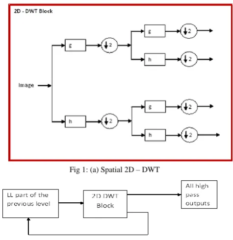
In this paper Low pass filter is represented as „h‟, and high pass filter as „g‟. The diagrammatical representation of the spatial DWT applied to images is as shown in figure 1 in which the input image is passed through the set of filters as discussed above. The multilevel spatial DWT needs repetitive such filters applied to the given images for multilevel resolution analysis [8]. Figure 1(a) represents the flow chart of single level spatial 2D-DWT, while figure 1(b) represents a generalized block diagram of 2nd and higher level 2D DWT applied to the image. For multi – level 2D-DWT, the image is passed through a series of high pass and low pass filters. The block diagram of figure 1(b) indicates a generalized method of estimating the high pass and low pass components of the image at higher levels of resolutions. This process of 2D-DWT is called as multilevel resolution analysis. It helps us to get finer details of the given image or signal. The outputs of DWT are arranged in specific order which helps to get details of the spatial as well as frequency components of the given image or signal.
Fig 1: (a) Spatial 2D – DWT
Fig 1: (b) Generalized block diagram of 2nd and higher level 2D DWT
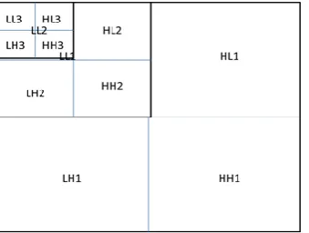
[image:1.595.316.554.467.712.2]Fig 2 (a): First level Column wise and Row wise decomposition of Spatial DWT
For higher level of 2D-DWT, the low pass outputs i.e. LL is taken into consideration for further decomposing e.g. LL1 component of level – 1 is used for level–2 2D-DWT and so on as shown in figure 2(b). This repetitive process can be done until the number of rows or number of columns of the LL part of higher level reaches to an odd number.
Fig 2 (b): Higher level Column wise and Row wise decomposition of Spatial DWT
This technique is applied on the images and also on videos by considering each frame as an image. Since frame by frame operation is memory inefficient and time consuming we go for another technique in which DWT is applied on the third axis along with rows and columns simultaneously. This is called as Temporal DWT technique and is explained in section II.
II. TEMPORAL DWT REPRESENTATION
[image:2.595.52.287.56.118.2]The temporal DWT is nothing but the DWT applied to the frames and is called as 3D – DWT, if it is applied along with the spatial 2D-DWT. This is the third axis where the DWT is applied i.e. first 2D-DWT on spatial domain and then 3D-DWT on the temporal domain. [3, 9].
Fig 3: Temporal DWT on Video
[image:2.595.333.542.146.234.2]The application of 3D-DWT leads to two components in the temporal domain these are called as high pass and low pass frames and are indicated in figure 3. With reference to figure 3, „1‟ indicates the high pass component of the level – 1 temporal DWT and „1L‟ represents the low pass component of the level-1 temporal DWT, „2‟ represents the high pass component of the level – 2 temporal DWT and „3‟ represents the low pass component of the level – 2
temporal DWT. Component 1L can be further decomposed by using temporal DWT. One thing to be observed from figure 3 is that the number of frames for every increased level of DWT are becoming half. Figure 3 represents the level-2(two level) temporal DWT only. There arrangement for storing point of view or representation point of view can be done as shown in figure 4 for further level of decomposition.[4].
Fig 4: Temporal representation of frames after application of 3D-DWT In figure 4, FP – 1 to FP – N represents the frame pointer for further processing or the frame pointer to get back the original frames. Further decomposition can be processed by application of 3D-DWT on the low pass frames i.e. on to the frames represented by „3‟. This process can be continued further till one reaches single or odd number of low pass frames remain at the output.
Reconstruction process of temporal DWT:
The reconstruction process of 3D-DWT involves the inverse DWT. This can be achieved by applying the IDWT on the components „2‟ and „3‟ initially and then with the result of this and with „1‟ the original video frames can be generated. Thus in general, to get back the original frames one need to apply the IDWT initially on to the latest decomposed outputs and along with this results one need to get back the original vide frames. This is very similar to the inverse DWT process applied to the images. Thus here one can perform the similar task of multilevel resolution process applied to the images on to the frames on temporal axis. Thus the frames will have multiple levels of processing. The process of reconstruction of IDWT is shown in figure 5 (a) and 5(b) taken together.
Fig 5(a): The first process of getting back the original video
Now by using the result (2 3)‟ and „1‟ we can get back the original video.
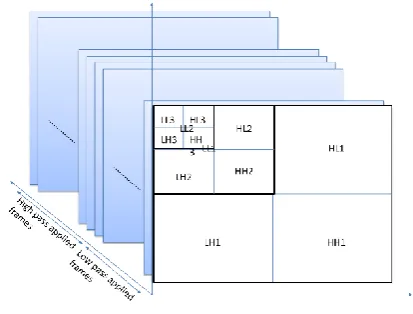
[image:2.595.92.262.218.346.2] [image:2.595.320.527.521.634.2] [image:2.595.46.293.544.682.2] [image:2.595.333.523.684.777.2]A normal video after applying the level-3 spatial 2D-DWT and level-1 temporal 2D-DWT is as shown in the figure „6‟.
Fig 6-Video after applying level-3 spatial DWT and level-1 Temporal DWT
The forward and reconstruction process explained in section-II is a general process of encoding and getting back the original video from the encoded video. The encoding and reconstruction mechanisms for the two mechanisms are quite different which will be discussed in section-IV. Along with the mechanisms we will also discuss about some of the equations which helps us in encoding and decoding the video in section-III.
III. EQUATIONS RELATED TO TEMPORAL DWT
Here we will discuss about the equations which help us in applying the K-level temporal DWT to the video. Here for explanation let us consider a video of size „m‟ by „n‟ by „p‟.
Equations for mechanism-1: Encoding:
(1)
Where,
„K‟ denotes the level of temporal DWT applied, „x‟ denotes the frame number and its maximum value
is ,
„F‟ denotes the frames of the original video. Decoding:
Where,
„K‟ denotes the maximum level of the temporal DWT applied,
„x‟ denotes the frame number and its maximum value is
„FP‟ denotes the low pass frames of the previous level.
To get back the frames of previous temporal level i.e., (K-1)th level, we need to know the high pass and low pass component of the present level i.e., Kth level. So, to get back the original video we have to start solving from Kth level, we cannot directly calculate the frames of any intermeddiate level without having the prior knowledge of the present temporal level.
Equations for mechanism-2: Encoding:
Where,
„Ks‟ denotes the level of spatial DWT applied,
„x‟ denotes the frame number and its maximum value
is ,
„Kt‟ denotes the level of temporal DWT applied, „F‟ denotes the frames of the original video. Decoding:
Where,
„Kt‟ denotes the maximum level of the temporal DWT applied,
„Ks‟ denotes the maximum level of the spatial DWT applied,
„x‟ denotes the frame number and its maximum value is
„FP‟ denotes the low pass frames of the previous level.
To get back the frames of previous temporal level i.e., (Kt-1)th level, we need to know the high pass and low pass component of the present level i.e., Ktth level. So, to get back the original video we have to start solving from Kt
th
level, we cannot directly calculate the frames of any intermeddiate level without having the prior knwledge of the present temporal level.
The equations (1),(2),(3) and (4) are applied only for the temporal DWT, for applying the spatial DWT the traditional method of DWT is followed[1]. If K-level temporal DWT is to be pplied at a constant spatial DWT level then replace the correponding level value in Ks in equations (3) and (4) and solve for the K level temporal DWT from equations (3) and (4).
IV. TWO DIFFERENT MECHANISMS APPLIED FOR VIDEO ENCODING AND DECODING
Mechanism- 1:
This mechanism can implement multi-level spatial 2D-DWT and the same level temporal 2D-DWT simultaneously [6].
Steps:
2. Now on the output of step-1 apply the temporal DWT of level-1.
3. From the output in step-2 all low pass component is taken and spatial 2D-DWT is applied on it, this is level-2 spatial 2D-DWT.
4. Now, on the output of step-3 temporal DWT is applied which is called as level-2 temporal DWT. 5. And for multi-level, this process is repeated until
the number of frames or number of rows or number of columns in all low pass component reaches to an odd number.
Now, the output frames are arranged in the manner as shown in figure 8. Now, the steps explained above are shown in the diagrammatical form in figure 7.
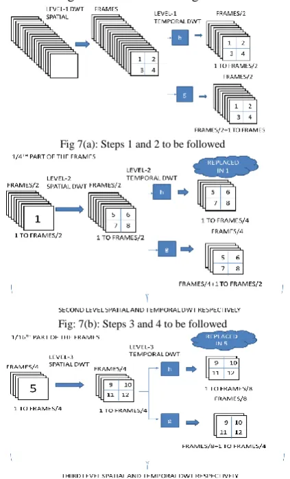
Fig 7(a): Steps 1 and 2 to be followed
Fig: 7(b): Steps 3 and 4 to be followed
Fig 7(c): Illustration of level-3 spatial DWT and level-3 temporal DWT After applying the mechanism-1 on videos they are arranged in the order as shown in figure 8 [4]. This arrangement will look like the multi resolution analysis applied on 3 axes i.e., row, column, and time [7]. So this mechanism can also be called as 3D multilevel pyramid decomposition [5].
Fig 8: Typical arrangement of the frames after the level-3 spatial DWT and level-3 Temporal DWT
Reconstruction process of the mechanism-1:
The reconstruction process is similar to the reconstruction process explained in section-II, but with slight changes. Now, we are going to discuss about the reconstruction mechanism, As mentioned in section-II reconstruction process start with the all low pass component of the highest DWT level. For the ease of explanation let us consider the video which is used in encoding process on which level-3 spatial DWT and level-3 temporal DWT are applied. The steps for reconstruction are as follows:
Steps:
1. Consider all low pass component of the highest DWT level. By using the high pass components of that level get back the all low pass component of the previous level. From the figure 7(c), all low pass component is „9‟ which is passed though low pass filter. By using the two outputs of the temporal DWT low pass and high pass get back the level-3 of spatial DWT. And by using „9‟ which is low pass and by using „10‟, „11‟, „12‟ which are high pass components, we can get back „5‟.
2. Now by using the output from step-1, apply the same procedure at the previous level to get the low pass component of its previous level. From the figure 7(b), the output obtained will be „1‟, which is the low pass component of the previous level. 3. This process is continued until the original video is
reconstructed.
These steps are shown in figure 9.
Fig 9(a): step-1
Fig 9(b): step-2
[image:4.595.63.275.211.560.2] [image:4.595.334.534.413.754.2] [image:4.595.65.266.649.763.2]processing of the higher levels in spatial and temporal DWT. This helps us in utilizing the memory efficiently as we are not processing 1/4th part of the frame and 1/2th part of the frame (with respect to the current frame size and number of frames) for every increase in the DWT level at the time of encoding. So the memory utilization will reduce by almost 3/4th when considered with the spatial DWT applied frame by frame and time consumption also reduces as we are computing less number of pixels in the increased level. In this way we can achieve the efficient utilization of the system memory and time requirement. Coming to the reconstruction, here also we are not utilizing the entire video at all levels. As we are approaching level-1 the usage of the system memory increases. So, at the time of reconstruction also one can achieve the efficient usage of system memory and time.
For a video of size „m‟ by „n‟ and with „p‟ number of frames. For the level-1 spatial and level-1 temporal DWT we require m*n*p bytes of system memory for processing the video. Now, when we are going to level-2 high pass components are not considered so we require (m/2)*(n/2)*(p/2) bytes of system memory for processing the video and if we go to next level further the memory requirement will be reduced by a factor of 8 for every increment in the DWT level of spatial and temporal DWT compared to the previous level.
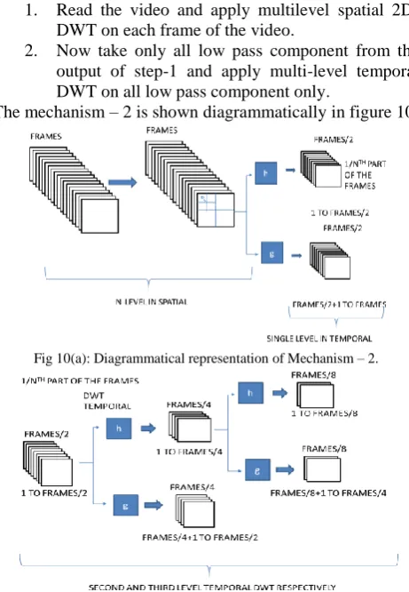
Mechanism-2:
This mechanism can implement multi-level spatial 2D-DWT and multi-level (may differ from spatial) temporal 3D-DWT.
Steps:
1. Read the video and apply multilevel spatial 2D-DWT on each frame of the video.
2. Now take only all low pass component from the output of step-1 and apply multi-level temporal DWT on all low pass component only.
The mechanism – 2 is shown diagrammatically in figure 10.
Fig 10(a): Diagrammatical representation of Mechanism – 2.
Fig 10(b): Diagrammatical representation of Mechanism – 2.
[image:5.595.312.560.54.220.2]Now, the output frames are arranged in the manner as shown in figure 11[4].
Fig 11: Arrangement of frames for further processing
In figure „11‟, SL represents corresponding spatial level indicated by number and TLH represents corresponding temporal level high pass component indicated by the number and TLL represents the all low pass component of the highest temporal DWT level applied (In figure 11 the applied DWT level is 3 for both spatial and temporal). Reconstruction Process:
Reconstruction process is similar to the process explained in section-II but with some minor modifications. The reconstruction process steps for mechanism-2 are discussed below:
Steps:
1. Consider the all low pass component of the highest level of temporal DWT applied and by using the high pass component of the same level get back the low pass component of the previous level. From figure 11, using TLL and TLH-3 get back the all low pass component of the previous level using the reconstruction process of the temporal DWT explained in section-II.
2. Now, by using the output in step-1 and high pass component of that level get the all low pass component of the previous level using the reconstruction process of temporal DWT discussed in section-II. From figure 11, using the output of step-1 and TLH-2 get the all low pass component of the previous level.
3. Repeat the steps 1 and 2 until all the temporal DWT levels applied on the video are completed. So, now we are left with the video on which only spatial DWT is applied.
4. Using the 2D-IDWT on the output of step-3, one can get back our original video.
[image:5.595.51.282.424.757.2]„m*n*p‟ number of bytes for processing the K-spatial DWT and bytes to process the temporal DWT.
V. RESULTS AND COMPARISION OF MECHANISMS
These two mechanisms which are implemented are tested on various standard videos, videos downloaded from internet and videos captured in the laboratory under non – standard conditions with a Canon Power shot A460 Digital camera having Approximately 5.3 Million Pixels 1/3.0 inch type CCD sensor with automatic exposure control and with video size of 448 by 640 pixels as given in table - 1. Here, we are presenting the comparison between the mechanisms, based on the time taken to transform and reconstruct the video in table 2 (for the temporal 1 and spatial level-1) and in table 3 for multi- level DWT (for spatial level-3 and temporal level-3). Along with the time the MSER [10] (Mean square error) value is also provided.
TABLE I.(VIDEOS USED FOR COMPARISION OF THE MECHANSIMS)
Video
No. Size
No. of Frames/ sec
TIME (in sec)
Total number of frames
Video 1 448 x 640 10 13 130
Video 2 240 x 320 29 17 493
Video 3 288 x 384 12 22 264
Video 4 144 x 176 30 12 360
Video 5 1080x1720 20 2 40
Video 6 120 x 160 15 8 120
Video 7 480 x 640 60 2 120
Video 8 480 x 640 10 12 120
TABLE II.(TIMING REQUIREMENTS AND MSER FOR SPATIAL LEVEL-1 AND TEMPORAL LEVEL-1)
Time &
MSER Mechanism-1
Mechanism-2
Video-1
DWT 4.34518 4.509034
IDWT 4.13382 3.401104
MSER 2.7899e-031 2.7899e-031
Video-2
DWT 4.942862 4.584396
IDWT 4.318520 3.621959
MSER 5.2875e-031 5.2875e-031
Video-3
DWT 3.576771 3.904889
IDWT 3.178713 2.738757
MSER 1.1818e-030 1.1818e-030
Video-4
DWT 1.157130 1.140782
IDWT 1.100707 1.010721
MSER 1.4371e-030 1.4371e-030
Video-5
DWT 230.158135 44.287551
IDWT 42.454580 20.464611
MSER 2.1324e-033 2.1324e-033
Video-6
DWT 0.613719 0.156875
IDWT 0.464239 0.137251
MSER 3.0632e-031 3.0632e-031
Time &
MSER Mechanism-1
Mechanism-2
Video-7
DWT 2.145582 2.343862
IDWT 1.907164 2.012581
MSER 7.1381e-032 7.1381e-032
Video-8
DWT 2.091870 2.373801
IDWT 1.868647 2.053528
MSER 2.8007e-031 2.8007e-031
TABLE III.(SPATIAL LEVEL-3 AND TEMPORAL LEVEL-3)
Time & MSER Mechanism-1 Mechanism-2
Video-1
DWT 5.358658 5.642298
IDWT 4.216121 3.472468
MSER 1.6972e-030 1.7414e-030
Video-2
DWT 6.256017 5.903929
IDWT 4.896240 3.673501
MSER 4.2157e-030 4.3378e-030
Video-3
DWT 4.837173 4.631625
IDWT 3.575453 3.085781
MSER 5.4270e-030 5.6075e-030
Video-4 DWT, IDWT,
MSER NA NA
Video-5
DWT 53.949063 11.185998
IDWT 18.928194 6.770777
MSER 7.0508e-033 7.2730e-033
Video-6
DWT 0.172794 0.212501
IDWT 0.135752 0.178058
MSER 1.2806e-030 1.2660e-030
Video-7
DWT 2.745044 3.674258
IDWT 2.182895 3.048072
MSER 4.1421e-031 3.8476e-031
Video-8
DWT 2.696968 3.688548
IDWT 2.149370 3.058648
MSER 1.5794e-030 1.6599e-030
NA: Not Applicable
Results:
TABLE IV.(COMPARISION OF RESULTS AT DIFFERENT DWT LEVELS)
Mechanism-1 Mechanism-2
Results for Video No. 6, frame No. 81 and DWT level as 2
Results for Video No. 7, frame No. 11 and DWT level as 3
Results for Video No. 8, frame No. 30 and DWT level as 2
Results for Video No. 8, frame No. 80 and DWT level as 2 Graphs:
Some of the graphs between the time taken for encoding, decoding and also for MSER values with respect to the DWT level applied are shown in fig 12-14.
VI. CONCLUSION
Thus, we conclude our paper by explaining the two mechanisms which can be used for video encoding with efficient utilization of system memory. One more important thing to be noted here is that, if we use 3D-EZW compression technique on encoded videos, then the compression factor would be very high.
Fig 12: Graph between MSER and DWT level for both mechanisms
Fig 13: Graph between time taken for encoding the video and DWT level for both mechanisms
Fig 14: Graph between time taken for reconstruction of the video and DWT level for both mechanisms
REFERENCES
[1] K.Sureshraju, V.R.Satpute, Dr.A.G.Keskar, Dr.K.D.Kulat, “Image Compression using wavelet transform compression ratio and PSNR calculations”, Proceedings of the National Conference on Computer society and informatics- NCCSI‟12, 23rd &24th april 2012.
[2] Nagita Mehrseresht and David Taubam, “An Efficient content adaptive motion-compensated 3D-DWT with enhanced spatial and temporal scalability”, IEEE Transactions on Image processing,VOL.15, No.6, JUNE 2006.
[3] Michael weeks and Magdy Bayoumi, “3-D Discrete Wavelet Transform Architectures”,0-7803-4455-3/98/$10.00 ©1998 IEEE. [4] G.Liu and F.Zaho, “Efficient compression algorithms for
Hyperspecral Images based on correlation coefficients adaptive 3D zero tree coding”, published in IET Image Processing, doi:10.1049/ict-ipr:20070139.
[5] Richard M.Jiang, Danny Crookes,”FPGA implementaiotn of 3D Discrete Wavelet Transform for real-time medical imaging”, 1-4244-1342-7/07/$25.00 © 2007 IEEE.
[6] O.Lopez, M.Martinez-Rach, P.Pinol, M.P.Malumbers, J.Oliver, “A fast 3D DWT video encoder with reduces memory usage suitable for IPTV”, 978-1-4244-7493-6/10/$26.00 © 2010 IEEE.
[7] Shadi Al Zu‟bi, Naveev Islam and Maysam Abbod, “3D Multi resolution analysis for reduced features segementation of medical volumes using PCA”, 978-1-4244-7456-1/10/$26.00 © 2010 IEEE. [8] Laura R.C.Suziki, J.Robert Reid, Thomas J.Burns, Gary B.Lamont,
Steven K.Rogers,”Parallel Computation of 3D-wavelets”.
[9] Anirban Das, Anindya Hazra, and Swapna Banerjee,“An Efficient Architecture for 3-D Discrete Wavelet Transform”, IEEE transactions on circuits and systems for video technology.
[image:7.595.39.297.46.459.2] [image:7.595.317.542.51.440.2] [image:7.595.50.280.619.787.2]