A method of estimating the average derivative: the multivariate case

Department of Economics University of Southampton Southampton SO17 1BJ UK

Discussion Papers in

Economics and Econometrics

A METHOD OF ESTIMATING THE AVERAGE DERIVATIVE, THE MULTIVARIATE CASE

Anurag N Banerjee

No. 0215

A Method of Estimating the Average Derivative, the

multivariate case.

Anurag N Banerjee

Department of Economics

University of Southampton

Southampton, UK

Abstract

The paper uses local linear regression to estimate the \direct" Average Derivative

± =E(D[m(x)]);where m(x) is the regression function. The estimate of± is the

weighted average of local slope estimates. We prove the asymptotic normality of the estimate under conditions which are di®erent from the conditions used by HÄ ardle-Stoker (H-S) (1989). Using Monte-Carlo simulation experiments we give some small

sample results comparing our estimator with the H-S estimator under our conditions

for asymptotic normality.

JEL codes: C13, C14, C15

Keywords: Semi-parametric estimation, Average Derivative, Linear regression

1

Introduction

Let (Yt;Xt),t= 1; : : : ; T be a multivariate sample from an unknown distributionF(y;x)

which is generated from the following model

Yt=m(Xt) +ut; t= 1; : : : ; T (1)

where m(x) is the unknown regression function, and the conditional expectation of ut

given Xt is zero, i.e. E(utjXt) = 0. We assume xis a l¡dimensional vector.1

Further, we assume that the regression functionm(x) is di®erentiable. We de¯ne the

average slope or the average derivative (A.D) of the regression functionm(x) as

± =

Z

D[m(x)]f(x)dx=E(D[m(x)]) (2)

where f(x) is the marginal density of X's andD[m(x)] is the ¯rst derivative ofm. We

can argue that± represents sensible "coe±cients" of changes in x. We can also show by

integrating by parts.

±=E(L(X)Y)

where L(X) =¡D[f(X)]=f(X).

The primary interest for Average Derivative Estimation (A.D.E) comes from the Gen-eral Index Model. where

m(x) =G(x0¯)

thenE(D[m]) =E(dG=d(x0¯))¯ is proportional to¯ ₈ x: So ±=E[dG=d(x0¯)]¯ =°¯; for some°;is proportional to¯. We can equivalently replace¯ byµ =¯=°, by normalising

asm(x) =G(x0µ) st. E[dG=d(x0µ)] = 1. Thus it can be interpreted as units of change in

y to changes in x. HÄardle and Stoker (1989) gives an application of it with a \Collision

Data".

The use of A.D in the context of Partial Index Models is also useful. For this x is

partitioned as (x(1);x(2)) into a l ¡ l vector of x(1) and l of vector x(2), and partition

± analogously as (±1; ±2). average derivatives will measure the true coe±cient when the

regressions obeys a Partial Index Structure ( Newey and Stoker (1989) ) if

m(x) = G(x0₍₁₎¯;x(2))

then ±1 equals ¯1 up to a scale. With an estimator ±b1 of ±1, we can extend the A.D.E

method to ¯tting a l+ 1 dimensional regression in the second stage, as ^G(x0₍₁₎±b1;x(2)). If

the model is multiple index form as

m(x) =G(x0₍₁₎¯1;x0(2)¯2)

then±2is likewise proportional to¯2(namely E[dG=d(x0(2)¯2)]). Again the A.D.E method

is easily extended.

A.D.E's are also used in speci¯c measurement problems in economics. A primary

ex-ample by HÄardle, Hilderbrand and Jerison (1991) is on measuring the positive de¯niteness

of the aggregate income e®ects matrix for assessing the "Law of Demand".

The A.D.E is used to estimate the following matrix.

±jj0 =E

Ã

dE(YjYj0jx) dx

!

where Yj = demand for the jth good andx = income level.

Further applications are suggested by the central role of derivatives in economic

mod-elling in form of marginal reactions and elasticities. Examples like pro¯t maximisation of

¯rms can be given. In this problem the ¯rm equate their marginal pro¯t derived from a

particular good to the price of that good. The average marginal reaction can be assessed

by the A.D estimate of the marginal pro¯t. One such example is given in Stoker (1992).

2

Method of Estimation.

Several methods have been suggested to estimate ±, the Average Derivative. HÄardle

and Stoker (1989) proposed an \indirect" estimate, ±bhs which is the sample analog of

E[L(X)Y]. This method estimates the covariance betweenL(X) andY, using consistent

non-parametric estimators of f(X) and D[f(X)]. Stoker (1991b) de¯nes the \direct"

Average Derivative Estimate, the sample analog of E(D[m(X)]) as±bd using the average

of the consistant non-parametric estimator ofD[m(X)]:Stoker also shows the asymptotic

equivalence of the \direct" and \indirect" estimators. The consistent estimates used in

the \direct" and \indirect" estimator are generally kernel estimators of the respective

We shall only assume some smoothness properties of the regression function and

mo-ment restrictions on the random variables which we state the next section. One important

di®erence in this method from the other methods is that there are no smoothness

assump-tions on the marginal density of X, i.e. f(x). We do assume that, the support of X is

the compact setS, without loss of generality it is assumed to be a subset of [0;1]l. Unlike

the HÄardle and Stoker method, the Fisher's information _L(X) may not exist. Therefore

the \indirect" estimator will not exist as well. For example suppose X is distributed

U[0;1], then L(X) does not exist. This case will not be covered by the method proposed

by HÄardle and Stoker. On the other hand if X is distributed with a Normal density we

cannot use our method since we assume the domain of f(x) to be a compact interval.

Though in this case we can use the HÄardle and Stoker method. So comparisons of our

two methods in terms of the asymptotics cannot be made and our methods complement

the HÄardle and Stoker method.

Let us motivate our method whenxis univariate. Without loss of generality, let S be the interval [0;1]: This interval is then partitioned, in equal intervals. We denote the

partition asP. Let the partition be 0 < t1 < t2 < : : : < tk¡1 <1, we denote (tr; tr+1] as

Hr (Hr is called a bin ). These bins are of equal size (jHrj=h). In the bins, which have

at least 3 observations we linearly regressYtonXt, st. Xt 2Hr. We denote the coe±cient

of the slope of the regression as ^¯r. This is a least squares estimate of the tangent of the

regression curvem(x), in the intervalHr.

We then take the an weighted average of the slopes in each of the binHr. The weights

are taken to be the average number of observations in the binHr.

Let us now generalise the idea when the dimension ofx is l:

Assume without loss of generality, the interval [0;1] is the domain of the marginal

density ofXi. We partition the domain, in equal intervals and denote the partition asPi.

Let the partition be 0< ti1 < ti2< : : : < ti(ki¡1) <1, we denote (t n

r; tnr+1] asHri (Hri is

called a bin in the xth_i dimension).These bins are of equal size (jHrij). The partition for

the whole of domain of f(x) is then P=P1£: : :£Pl where Hr =Hr1£: : :£Hrl is the

bin to be considered in this l_¡dimensional space. Notice the number of bins is now at

most k = k1£: : :£kl: We shall only consider those bins such that Hr ½ S: Note that

rest of the method is similar to the univariate case.

Suppose we have atleastp _¸l+ 2 points in Hr, we linearly regress yt onxt as

yt= ®r+¯r0xt , s:t Xt2Hr:

We denote the estimate coe±cient of the slope of the regression,¯r as

^

¯r = [Srx]¡

1XT

t=1

(xt¡x¹r)Ifxt 2Hrgyt

where Sr x =

T

X

t=1

(xt¡x¹r) (xt¡x¹r)TIfxt 2Hrg

and ¹xr =

1 T

T

X

t=1

xtIfxt2Hrg:

This is a least squares estimate of the tangent of the regression curve m(x), within the

interval Hr.

We then take the an weighted average of the slopes in each of the binHr. The weights

are taken to be the average number of observations in the binHr, denoted by

wr=

1 T

T

X

t=1

Ifxt 2Hrg:

where I is the indicator function.

De¯nition 1 We de¯ne our Average Derivative estimator as

^ ± =

k

X

r=1

wr¯brIfTr ¸pg

where Tr=wrT, the number of observations in the rth bin and k is the number of bins.

Note that in de¯nition (1), we assume that if there are insu±cient number of

observa-tions to regress, the observaobserva-tions in the bin contribute nothing to the Average Derivative

Estimate.

We will show, under some assumptions made later that asymptotically

p

T(^±¡±) 'N³0; V arfm0(X)g+¾_u2§¡1´;

where ¾2

u is the variance of ui's and § is the variance-covariance matrix of X.

We also show that the large sample variance V arfm0(X)g+¾2u§¡1can be consistently

De¯nition 2 We de¯ne the estimated variance of ^± as

^ V =

k

X

r=1

wr¯^r¯^r

0

I_fTr ¸pg ¡±^±^0

3

Distributional properties and comparison with HÄ

ardle-Stoker Estimator.

3.1

Large Sample Results

We shall now prove some large sample results under the following assumptions

A1 The support of f(x) is the compact set S ½ [0;1]l and f(x) is uniformly bounded

above by a constantC, for some C >0.

A2 The second derivative of m(x),D2_{[m];exists and bounded.}

A3 The variance ofut isE(u2tjXt) =¾2u, exists and is bounded.

A4 As T ¡! 1,

p

T h_¡! 0 and log(T)

T h ¡!0:

We will make some brief comments on the assumptions. The ¯rst assumption (A1) is

not a popular assumption is the non-parametric econometrics literature. This assumption

of f(x) > 0 is necessary to ensure that there is atleast p_¡observations in each bin to

perform the required regression (in large sample). However we also want the density to

be bounded above since we do not want to put too much weight on any particular ^¯r:

The smoothness assumption of the regression function (A2) is also necessary for the same

reason. Assumption three (A3) is a standard assumption for linear models. Finally the

last assumption (A4) ensures that the size of the bins shrinks at the rate of pT ; but

the size should not get too small too quickly (log(T)=T h _¡!0) otherwise there will be

insu±cient number of observations in the bin to do a regression.

Theorem 1 Under the stated assumptions A(1) to A(4) we have the following

p

where b± is the A.D.E de¯ned in De¯nition 1.

The interesting thing to observe here is that if m(x) is linear (i.e. m(x) = ®+¯0x)

then the asymptotic variance coincides with the asymptotic variance of the classical Least

Squares estimator of¯. Note that in case ofm(x) being linear, ±=¯. So in this particular

case we get a standard classical result. This implies that in the case of linearity we will

not lose e±ciency when compared to the Least Square Estimation method.

Theorem 2 Under the assumptions A(1) to A(4) we have the following

c

V_!P V ar(D[m(X)]) +¾2

u§¡1

where cV is the estimated variance of b± as de¯ned in De¯nition 2.

Theorem (2) facilitates the measurement of precision of ^±as well as the inference on

hy-potheses about±. For instance, getting interval estimates using the estimated covariance

matrix of±;b cV.

Moreover, consider testing restrictions ofHo :± =±0. Tests of this hypothesis can be

based on the Wald type W statistic

W = ³b±¡±o

´₀ c

V¡1³±b¡±o

´

(3)

which will have a limiting Â2 _{distribution.}

As a practical application, since we do not require the density f(x) to vanish, our

method can be used to test for linearity or stability by dividing the data into di®erent

regions and calculating the ADE of each region and testing for equality like a Chow test

using (3).

3.2

Small Sample Results

We will now study the small sample properties of our estimator and compare it with

the Hardle Stoker Estimator. We do so by using Monte Carlo simulations on a model

Model

We study a univariate model as described below,

m(x) = 1_¡x+x2

u _» N(0; ¾_u2)

X » U[0;1]

Therefore, for this model:

± = 0

and

V ar_fD[m(x)]_g+¾2

u§¡1=

1 3+ 12¾

2

u

Let us describe the algorithm for computing our estimate.

Algorithim

Step(0) Generatef(Xt; Yt)gT_t=1 from the model.

Step(1) Choose the size of the bin such that it satis¯es A(4).

Step(2) Divide the domain into k parts as described before.

Step(3) Compute the Least Square Estimate, ^¯rwith at least 3 observations in each bin,

Hr. Compute the ratio #0fXt2Hrg=T =wr. Multiply and get ^¯rwr.

Step(4) Add ^¯rwr over all bins, Hr and get the estimate ±.

Choice of Bin Size.

As observed before the size of the bin is inversely proportional to the number of partitions.

We describe here an adhoc method of choosing h from the data size (T). We will use

A(4) and the \de¯nition of limit" to choose our bin width. We have,

p

T h_¡!0 and log(T)

implies given ² > 0 , ₉ T st. for T _¸ T p _{T h} ², and from these two

inequalities we have

log(T) T ² h

²

p

T

From this we ¯xh as follows. Taking equalities on both sides, we have

log(T) T ² =

²

p

T log(T)1=2

T1=4 = ²

so we get

h= log(T)

1=2

T3=4

so

k =

2 6 4

v u u

t T

p

T log(T)

3 7 5

Simulations and Descriptive Statistics.

We generate s (= 1000) datasets of size T (= 50;200;400) from the model we consider.

Then with these data sets we estimate ± with the method described before and get the

estimated value of ± (^±T). We will denote by ±bT(i) as the estimated value of ± of the

ith _{simulation (i.e. with the i}th _{dataset). With these ±b}

T(i) we calculate the following

summary descriptive statistics, to show how the estimator behaves. We shall now give a

brief description of the summary statistics.

Mean of±bT(i)0s = ±bT =

1 s

s

X

i=1 b

±T(i)

Variance of ±bT(i)0s = V(±bT) =

1 s

s

X

i=1

(b±T(i)¡±bT)2

MSE of ±bT(i)0s = M SE(±bT) =

1 s

s

X

i=1

(±bT(i)¡±)2

Further more we will look at the estimate of the Pr(_¡p3

T p

V +± ±bT p3_T p

V +±),

where V = V ar(D[m(X)]) +¾2_u=¾_x2. This is a natural statistic to look at, since by the

Theorem in the previous section we know that

Pr(¡p3

T

p

V +± ±bT

3

p

T

p

V +±)asy» ©(¡p3

T

p

V +± ±bT

3

p

T

p

for large T.

So we can look at the following estimate of the above probability as

c

Pr = 1 s

s

X

i=1

I(¡p3

T

p

V +± ±bT(i)

3

p

T

p

V +±)

This probability gives us an estimate of how accurately our±bT estimates±in small samples.

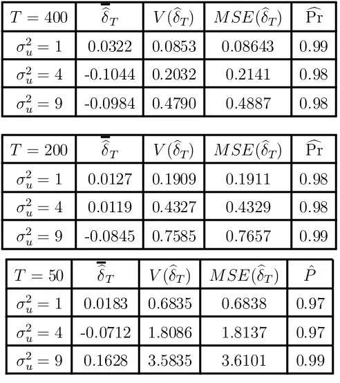
Results

In the model described before, we vary the error variance (¾2

u = 1;4;9), so as the

dis-turbance of the error increases we expect to see a larger variation about the mean of the

estimates±bT and the actual±(± = 0 in this model). The results are tabulated in Table 1.

We see as expected with the decrease of sample size the variation increases. The closeness

of V(±bT) and MSE(±bT) tells us that our ±bT's are close to the actual, with increasing ¾u2

and sample size T.

[T able1]

3.3

Comparisons with HÄ

ardle-Stoker Method

The HÄardle-Stoker method (1989) uses the indirect estimate

b

±hs =

1 T

T

X

t=1

yt

d

Dfh(xt)

b

fh(xt)

where fbh(xt) and Dfdh(xt) are the kernel density estimates with a bandwidth h: It has

been shown in (HÄardle-Stoker 1989) that under some assumptions

p

T³±bhs¡±

´asy

¼ N³0; V ar(D[m(X)]) +¾_u2E(L(X))2´ (4)

when the error term u is uncorrelated with X: In his article, Stoker (1991b), de¯nes the

"direct" estimator of± de¯ned as

b

±d =

1 T

T

X

t=1

D[cm(xt)]I

³ b

fh(xt)> b

´

where mc(xt) is the (Nadaraya-Watson) kernel regression estimator of m(x); is

the H-S estimator, pT ³±bd¡±

´

has the same asymptotic distribution as in (4). Given

this we shall compare only the ±bhs estimator with our proposed ±:b

Comparing the asymptotic variances of the±bhs or ±bd(4) and the asymptotic variance

of ±b (Theorem 1), we see that by Rao-Cramer inequality,

V ar(D[m(X)]) +¾2_uE(_L(X))2> V ar(D[m(X)]) +¾_u2§¡1:

But does this implies that ±bis asymptotically more e±cient than±bhs or b±d ? The answer

to that question is not necessarily so, since assumption (A1) used to derive the asumptotic

violates the assumption of smoothness off needed for the asymptotic normality of

HÄardle-Stoker A.D.E 2_{. Also H-S assumptions on f violates assumption A1, since we need the}

assumption of compact support off for asymptotic normality of ±:. Hence they can onlyb be compared through simulation methods.

We use the same model as in (4) 3_{. To compute the H-S estimator bandwidth of the}

Kernel,h is taken to be T¡2=7_{, the optimal bandwidth obtained by minimising the MSE}

(HÄardle, Hart, Marron and Tsybakov (1991)). We use the Gaussian Kernel to compute

the density.

[T able2]

Generally as expected our proposed A.D.E ±b out performs ±bhs in this simulation, the

reason being that model violates the condition for asymptotic normality of ±bhs: So our

estimator complements the H-S estimator.

4

Conclusion

The paper proposes an alternative method of estimating the Average Derivative Estimate

(A.D.E). We propose the method of averaging the local OLS slopes to estimate the A.D.E.

We prove the asymptotic normality of our A.D.E under some regularity assumptions.

These assumptions are similar but not same as the assumptions under which HÄardle-Stoker

2_{Assumption 1,f(x) = 0;at the boundary of the support and.assumption 5 all derivatives off(x) of}

orderl+ 2;exists. (HÄardle-Stoker, 1989)

3_{Notice that the assumption that X»U(0;1) violates the assumption of smoothness off needed for}

(H-S) proved the (asymptotic) normality of their A.D.E. Stoker (1991b) also de¯nes a

"direct" estimator of±; and shows the assymptotic equivalence of the direct and the

H-S estimator. The H-H-S estimator requires some smoothness conditions on the density of

explanatory variable f(x):Our method we do not require such assumptions but we need

f(x) to have compact support. It might be worthwhile to point out that by not requiring

the density f(x) to vanish, our method can be used to test for linearity or stability by

dividing the data into di®erent regions and calculating the ADE of each region and testing

for equality like a Chow test.

The method described, is applied to a model with single regressor, assuming the

density of x to be uniform. We simulate and compare the small sample results of H-S

estimator with our estimator using various measures of performance. The results also

indicate that our estimator performs better than H-S estimator under the given situation

where asymptotic conditions of the HÄardle Stoker method is not strictly applicable. Our

References

Ahn, H, 1997, Semiparametric Estimation of a Single-Index Model with

Nonparametri-cally Generated Regressors Econometric-Theory; Vol 13(1), pp 3-31.

Banerjee, A.N, 1994, A Method of Estimating the Average Derivative, Universite Catholique

de Louvain CORE Discussion Paper: 9403.

HÄardle, W, 1992, Applied Non Parametric Regression, Cambridge, Cambridge University

Press (Econometric Society Monographs).

HÄardle, W., W.Hilderbrand. and M.Jerison, 1991, Emperical Evidence for the Law of

Demand, Econometrica, Vol 59, pp 1525-1550.

HÄardle, W, and T.M.Stoker, 1989, Investigating Smooth Multiple Regression by the

Method of Average Derivatives, Journal of American Statistical Association, Vol 84, 408, pp 986-995.

HÄardle, W, J.Hart, J.S.Marron, and A.B.Tsybakov, 1992, Bandwidth Choice for Average

Derivative Estimation, Journal of the American Statistical Association, Vol 87, 417,

pp. 218-226

Newey, W.K and T.M. Stoker, 1993, E±ciency of Weighted Average Derivative

Estima-tors and Index Models, Econometrica, Vol 61, pp 1199-1223

Rao, C.R., 1973, Linear Statistical Inference and its Applications, (John Wiley, New

York).

Ser°ing, R.J, 1980, Approximation Theorems of Mathematical Statistics, (John Wiley,

New York).

Stoker, T.M., 1991a, Lectures on Semiparametric Econometrics, (CORE Lecture Series,

Core Foundation, Louvain-la Neuve).

Stoker, T.M, 1991b, Equivalance of Direct, Indirect and Slope Estimators of

Statistics, W.A. Barnett, J,Powell and G, Tauchen, eds., Cambridge University

Tables

Table 1: Simulation results:

T = 400 ±bT V(±bT) M SE(±bT) Prc

¾2

u= 1 0.0322 0.0853 0.08643 0.99

¾2

u= 4 -0.1044 0.2032 0.2141 0.98

¾2

u= 9 -0.0984 0.4790 0.4887 0.98

T = 200 ±bT V(±bT) M SE(±bT) Prc

¾2

u= 1 0.0127 0.1909 0.1911 0.98

¾2

u= 4 0.0119 0.4327 0.4329 0.98

¾2

u= 9 -0.0845 0.7585 0.7657 0.99

T = 50 ±bT V(±bT) M SE(±bT) P^

¾2

u= 1 0.0183 0.6835 0.6838 0.97

¾2

u= 4 -0.0712 1.8086 1.8137 0.97

¾2

u= 9 0.1628 3.5835 3.6101 0.99

Table 2: Comparison with HÄardle-Stoker method

T = 100 ±bhs ±b M SE(±bhs) M SE(^±)

¾2

u= 1 -1.128 0.0575 3.8334 0.2003

¾2

u= 4 1.6077 -0.0328 2.6459 0.6492

¾2

u= 9 -0.1951 -0.1951 4.2662 1.4613

where

Mean of±bhs(i)0s = ±bhs=

1 100

100 X

i=1 b

±hs(i)

MSE of ±bhs(i)0s = M SE(±bhs) =

1 100

100 X

i=1

Appendix.

Lemma 1 Under the assumptions, we have as T _{! 1};

1) sup

1<r<k

T¡14 ° ° ° ° ° 1 T T X t=1

xtx0tIfxt2Hrg ¡pr¹2 ° ° ° ° ° P !0 2) sup 1<r<k

T¡14 ° ° ° ° ° 1 T T X t=1

xtIfxt2Hrg ¡pr¹1 ° ° ° ° ° P !0 3) sup 1<r<k

T¡14 ° ° ° ° ° 1 T T X t=1

xtutIfxt 2Hrg

° ° ° ° ° P ! 0 4) sup

1<r<kT

¡1 4 ° ° ° ° ° 1 T T X t=1

utIfxt2Hrg

° ° ° ° ° P !0 5) sup

1<r<kT

¡1 4 ° ° ° ° ° 1 T T X t=1

I_fxt2Hrg ¡pr

° ° ° ° ° P !0 where

pr =

Z

Hr

f(x)dx; ¹₁=E(xt) and ¹2= E(xtx0t):

Proof of Lemma 1: Observe that, if Mr;(1 r k) are a collection of independent

random variables then,

Pr

(

sup

1<r<kkMrk> "

)

= 1_¡

k

Y

r=1

(1_¡Pr (_kMrk> "))

so

Pr

(

sup

1<r<kk

Mrk> "

) !0 iif k Y r=1

(1¡Pr (kMrk> "))!1

iif

k

X

r=1

Pr (kMrk > ")!0

if

k

X

r=1

EkMrk2! 0 (using Chebyshev's inequality) (5)

1) Let Mr=T¡

1 4 1

T

P_T

t=1(xtx0tIfxt 2Hrg ¡pr¹2); so

E_kMrk2= p T E ° ° ° ° ° 1 T T X t=1

(xtx0tIfxt2Hrg ¡pr¹2) ° ° ° ° ° 2 p T 1 T2E

° ° ° ° ° T X t=1

xtx0t(Ifxt2 Hrg ¡pr)

° ° ° ° ° 2 +E ° ° ° ° °pr

à 1 T T X t=1

xtx0t¡¹2 !°°_° ° ° 2 p T 1 T2E

° ° ° ° ° T X t=1

xtx0t(Ifxt2 Hrg ¡pr)

° ° ° ° ° 2

+p2_rE

° ° ° ° °pr

à 1 T T X t=1

xtx0t¡¹2 !°°_° ° ° 2 p T 1 T2E

à _T

X

t=1

kxtx0tk jIfxt2Hrg ¡prj

!2

+p2

rE ° ° ° ° ° Ã 1 T T X t=1

xtx0t¡¹2 !°°_° ° ° 2 p T 1

T2ConstE

à _T

X

t=1

jIfxt2Hrg ¡prj

!2 0

B

@ (sincext's are bounded

andE(xtx0t) =¹2

1 C A

=pT 1

T2C onst 2 6 4

PT

t=1E(Ifxt 2Hrg ¡pr)2

+PT

t<t0₌₁EjIfxt 2Hrg ¡prjEjIfxt2Hrg ¡prj

3 7 5

(since xt's are independent)

=pT 1

T2C onst h

T pr(1¡pr) +

³_T 2 ´

(2pr(1¡pr))2

i

Const:

"

1

p

Tpr+pr

p

T h

#

:

Therefore summing overr we get

k

X

r=1

E_kMrk2 < Const:

" 1 p T + p T h # :

Hence asT _{! 1}, the expression above goes to zero since pT h_!0:

The proofs of 2) 3) 4) and 5) are similar to 1).

Lemma 2 Assume A(2) and A(4), if Tr ¸p then ,

^

¯r =D[m( ¹xr)] +R(1)r + µr

where,

sup

1 r k

R(1)

r P

=o³T¡12 ´

and µr = [Srx]¡

1XT

t=1

Proof of Lemma 2: We have

^

¯r = [Srx]¡

1X

t2Ir

e

xt;ryt= [Srx]¡

1X

t2Ir

e

xt;rm(xt) +µr;

wherexet;r = (xt¡x¹r)Ifxt 2Hrg and Ir =ft:xt2Hrg:

Take a Taylor series expansion around ¹xr of m(xt);for those xt 's which are in Hr:

m(xt) = m( ¹xr) +xe0_t;rD[m( ¹xr)] +

1 2xe

0

t;rD

2

[m(»tr)]xet;r

for some »tr betweenxt and ¹xr: Therefore

[Sr x]¡1

X

t2Ir

e

xt;rm(xt) =D[m( ¹xr)] +R(1)r

where

R(1)r =

1 2

"

Sr x=T

tr(Sr x=T)

#_¡1P

t2Irxet;rxe T

t;rD2[m(»tr)]xet;r

tr(Sr x)

and

Srx =

X

t2Ir

e

xt;rxe0t;r

using the previous lemmas. Taking the norm

Note that by lemma (1), we have

1 TS

r x

P !pr

³

¹_2¡¹2 1 ´

=pr§

therefore

tr

µ₁

TS

r x

¶

P

!prtr(§)

combining we get

Srx=T

tr(Sr x=T)

P

! _tr§_(§)

"

Sr x=T

tr(Sr x=T)

#_¡1

P !

"

§ tr(§)

#_¡1

P

Also

° °

°Pt2Irxet;rxe0t;rD

2_[m(»

tr)]xet;r

° ° °

tr(Sr x)

P

t2Irkxet;rk

° °

°ex0_t;rD2_[m(»

tr)]xet;r

° ° °

tr(Sr x)

P

t2Irkxet;rk

° ° °ex0t;rxet;r

° ° °

tr(Sr x)

C onst

p

T h

P

t2Ir

° °

°ex0_t;rxet;r

° ° °

tr(Sr x)

Const

=O³pT h´

Hence R(1)

r P

=o³pT´ since by assumptionpT h_! 0:

Lemma 3 We have for a given p;

k

X

r=1

wrD[m( ¹xr)]IfTr > pg =

1 T

T

X

t=1

D[m(xt)] +R(2)+R(3)

where R(2)_{; R}(3) ₌P _o³_T¡1 2

´

:

Proof of Lemma 3: Let us de¯ne

R(2)=

k

X

r=1

wrD[m( ¹xr)]IfTr > pg ¡ k

X

r=1

wrD[m( ¹xr)]IfTr >0g

R(3)=

k

X

r=1

wrD[m( ¹xr)]IfTr >0g ¡

1 T

T

X

t=1

D[m(xt)]

then

k_X(T)

r=1

wrD[m( ¹xr)]IfTr> pg=

1 T

T

X

t=1

D[m(xt)] +R(2) +R(3)

We shall now showR(2)_{; R}(3) ₌P _o³_T¡1 2 ´

° ° °R(2)

° ° °= ° ° ° ° ° k X r=1

wrD[m( ¹xr)] (IfTr > pg ¡IfTr >0g)

° ° ° ° ° = ° °° ° ° k X r=1

wrD[m( ¹xr)]Ifp > Tr >0g

° °° ° ° M1 ° ° ° ° ° k X r=1

wrIfp > Tr >0g

where M1 is the upper bound for D[m( ¹xr)]: Since the random variablePkr=1wrIfp >

Tr>0g is positive we have to show that

E

à _k

X

r=1

wrIfp ¸Tr>0g

! !0 therefore E Ã _k X r=1

wrIfp¸Tr>0g

!

=

k

X

r=1

E(wrIfp¸Tr >0g)

= 1 T

k

X

r=1

E(TrIfp¸Tr >0g) =

1 T k X r=1 p X j=1

jpj_r(1¡pr)T¡j

= 1 T k X r=1 pr 8 < : p X j=1

jpj¡1

r (1¡pr) T¡j

9 = ;

Since Ppj=1jprj¡1(1¡pr)T¡jis bounded we have

E

à _k

X

r=1

wrIfp > Tr>0g

!

=O³T¡1´

hence°°°R(2)°°_°=o(T¡1₎

Now let us consider

° °

°R(3)°°°=

° ° ° °° k X r=1

wrD[m( ¹xr)]IfTr>0g ¡

1 T

T

X

t=1

D[m(xt)]

° ° ° °° ° ° ° ° ° ° k X r=1 wr 0

@_{D[m( ¹xr)]¡} 1

Tr

X

i2Ir

D[m(xt)]

1

A_IfTr>0g ° ° ° ° ° ° k X r=1 wr ° ° ° ° ° ° 1 Tr X

i2Ir

(D[m( ¹xr)]¡D[m(xt)])

° ° ° ° °

°IfTr>0g

k X r=1 wr 1 Tr X

i2Ir

° °

°D2h_m(»0

t;r)i°°°kxt¡x¹r)kIfTr >0g

=O 0 @ k X r=1 wr 1 Tr X

i2Ir

kxt¡x¹r)k

1 A =O Ã _k X r=1

wrh

!

=O(h) (Since

k

X

r=1

wr= 1)

then°°°R(3)°°_°=o³_T¡1 2 ´

since by assumption h= o³T¡12 ´

Lemma 4 Under the assumptions, we have

sup

1<r<k p

T°°°µr¡§¡1Sxu

° ° °!P 0

where

µr = [S_xr]¡1 T

X

t=1

(xt¡xt)Ifxt2Hrgut

and Sxu =

1 T

T

X

t=1

(xt¡xt)ut:

Proof of Lemma 4: We have,

µr= [Srx]¡

1

S_xur

=

2

41

Tr

X

t2Ir

e

xt;rxeTt;r

3 5 ¡1 1 Tr T X t=1 e

xt;rut

where

e

xt;r= (xt ¡xt)Ifxt2Hrg

This can be written as

1 wr

Sr_x

¸¡1

1 wr 1 T T X t=1 e

xt;rut

we have from previous lemmas

Sr x

T

P

=pr§ and wr=P pr

by assumption aspr >0;for all rand § is positive semi-de¯nite, we have

1 wr

Sr x

¸¡1

P

!§¡1_{; uniformly (6)}

also notice that

p

T 1 T2E

° ° ° ° ° 1 T T X t=1

xtutIfxt 2Hrg ¡

1 T

T

X

t=1

xtutpr

° ° ° ° ° 2

=pT 1 T2E

à _T

X

t=1k

xtk jIfxt 2Hrg ¡prjut

!2

p

T 1

T2Const 2 6 4 PT t=1 h

E(I_fxt2Hrg ¡pr)2E(u2tjxt)

i

+PT_t<t0₌₁E[jIfxt 2Hrg ¡prjEjIfxt2Hrg ¡prjE(jutut0jjx_t)]

following similar steps in the proof of lemma (1)

p

T 1 T2E

° ° ° ° ° 1 T T X t=1

xtutIfxt2Hrg ¡

1 T

T

X

t=1

xtutpr

° ° ° ° ° 2 =O Ã 1 p

Tpr+pr

p

T h

!

since E(u2_tjxt) and E(jutut0jjx_t) are bounded. Therefore

1 p T k X r=1 E ° ° ° ° ° 1 p T T X t=1

xt(Ifxt2Hrg ¡pr)ut

° ° ° ° ° 2 =O Ã 1 p T + p T h !

Using the same techniques as in lemma 1, we proof that

sup 1<r<k ° ° ° ° ° 1 T T X t=1

xtutIfxt 2Hrg ¡pr

1 T

T

X

t=1

xtut

° ° ° ° ° P !0

we can proof similarly for

sup 1<r<k ° ° ° ° ° 1 T T X t=1

xtIfxt 2Hrg ¡pr

1 T T X t=1 xt ° ° ° ° ° P !0 Therefore sup

1<r<kk

S_xur ¡Sxuk !P 0

Combining with (6) we get the result.

Lemma 5 Under the assumptions,

p

T

k

X

r=1

wrµrIfTr > pg D

!N³0; ¾2_u§¡1´:

Proof of Lemma 5: Using the previous lemma we can show that

p

TµrIfTr> pg=P p

T§¡1SxuIfTr > pg+ p

T R(4)

r ;

where sup1 r kR(4)r P

= o³T¡12 ´

: After multiplying and both sides by w0_rs and summing

across all the bins we have

p

T

k

X

r=1

wrµrIfp > Trg=P p

T§¡1Sxu k

X

r=1

wrIfTr > pg+ p

T

k

X

r=1

wrIfTr > pgR(4)r :

We can easily show that¯¯¯Pkr=1wrIfTr> pg ¡1

¯ ¯

¯!P 0;and since

° ° ° ° ° k X r=1

wrIfTr > pgR(4)_r

° ° ° ° ° ° ° ° °

°1supr kR

We have °°°Pkr=1wrIfTr > pgR(4)r

° ° ° !P 0:

Observe that by central limit theorem and asu !P 0 we have,

p

T Sxu =

1 p T T X t=1

(xt¡¹1)ut¡ p

T(xt¡¹1)u

D

=N³0;§¾2´_:

Therefore

p

T§¡1Sxu =D N

³

0;§¡1¾2´:

giving us p T k X r=1

wrµrIfTr > pg !D N

³

0; ¾2

u§¡1

´

:

Proof of Theorem 1: From lemma (2) we can write

p

T±b=pT

k

X

r=1

wr¯brIfTr > pg

=pT

k

X

r=1

wr

³

D[m( ¹xr)] +R(1)r

´

IfTr> pg+ p

T

k

X

r=1

wrIfTr > pgµr

where sup1 r kR(1)r P

=o³T¡12 ´

(since by assumptionpT h_! 0):ThereforePkr=1wrR(1)r IfTr >

p_g=P o³T¡1 2 ´

:Further using lemma 3 we can write

p

T

k

X

r=1

wrD[m( ¹xr)]IfTr > pg=P

1 p T T X t=1

D[m(xt)] + p

T R(2)₊p_{T R}(3)_:

As ³pT R(2)_;p_{T R}(3)_;Pk

r=1wrR(1)r IfTr> pg

´ _P

=o³T¡12 ´ ;we have p T k X r=1

wr¯brIfTr > pg P

= p1

T

T

X

t=1

D[m(xt)] + p

T

k

X

r=1

wrIfTr> pgµr:

Using central limit theorem we show that

1 p T T X t=1

D[m(xt)]=D N(0; V ar(D[m(x)]))

and by lemma (5) we have

p

T

k

X

r=1

wrµrIfTr > pg !D N

³

Since Pk

r=1wrµrIfTr > pgand p1_T PTt=1D[m(xt)] are uncorrelated by assumption, we

prove that

p

T

k

X

r=1

wr¯brIfTr > pg !D N

³

0; V ar(D[m(x)]) +¾_u2§¡1´

Proof of Theorem 2: We shall use lemma (2) and the fact that x_! xx0 is continuous

mapping, to show that

b

¯_r¯b0_r=P D[m( ¹xr)]D[m( ¹xr)]0+µrµ0_r:

Then we use the proof of lemma (3) and the factD[m( ¹xr)]D[m( ¹xr)]0 is di®erentiable to

get

k

X

r=1

wr¯br¯b

0

rIfTr > pg=P

1 T

T

X

t=1

D[m(xt)]D[m(xt)]0+ k

X

r=1

wrµrµ0rIfTr > pg

By weak law of large numbers we have,

1 T

T

X

t=1

D[m(xt)]D[m(xt)]0 P

!E³D[m(x)]D[m(x)]0´

As in lemma (4) we can show that

sup

1<r<kT

° °

°µrµ0r ¡§¡1SxuSxu0 §¡1

° ° °!P 0;

and again by weak law of large numbers we have,

T SxuSxu0 P

!¾u2§ asE(SxuSxu0 ) =¾u2§

implying

sup

1<r<k

° °

°Tµrµ0r¡¾2u§¡1

° ° ° !P 0

Therefore

k

X

r=1

wrµrµ0rIfTr > pg =P ¾u2§¡1 k

X

r=1

wrIfTr > pg

P

= ¾2

u§¡1since k

X

r=1

From previous theorem we also know that

b

±_!P± =E(D[m(x)])

Hence

c